Revisiting the critical behavior of nonequilibrium models in short-time Monte Carlo simulations

Abstract

We analyze two alternative methods for determining the exponent $z$ of the contact process (CP) and Domany-Kinzel (DK) cellular automaton in Monte Carlo Simulations. One method employs mixed initial conditions, as proposed for magnetic models [Phys. Lett. A. 298, 325 (2002)]; the other is based on the growth of the moment ratio $m(t)=\langle\rho^{2}(t)\rangle/\langle\rho(t)\rangle^{2}$ starting with all sites occupied. The methods provide reliable estimates for $z$ using the short time dynamics of the process. Estimates of $\nu_{||}$ are obtained using a method suggested by Grassberger.

I Introdution

The dynamics of spin models quenched from high temperature to the critical point is a subject of considerable current interest, because the initial phase of the relaxation (the so-called short time dynamics) carries important information about static and dynamic critical behavior. Using a phenomenological renormalization group analysis, Janssen, Schaub and Schmittmann Janssen demonstrated the scaling law

$$\left\langle M\right\rangle(t)\sim m_{0}t^{\theta}$$ (1)

characterized by the new critical exponent $\theta$. (Here $\left\langle\cdot\right\rangle$ denotes an average over initial configurations consistent with initial magnetization $m_{0}$, and over the noise in the stochastic dynamics.) Relation (1) holds for times $t<t_{\max}\sim m_{0}^{-z/x_{0}}$, where $z$ is the dynamic exponent, while $m_{0}$ denotes the initial magnetization, and $x_{0}$ its anomalous dimension. The “critical initial slip” described by Eq. (1) emerges from an initially disordered state, and is characteristic of a stochastic, far from equilibrium relaxation process. This approach also offers a way to determine the static critical exponents, since the scaling law used to deduce Eq. (1) can also be applied to higher moments of the order parameter, yielding:

$$\left\langle M^{k}\right\rangle(t,m_{0})=L^{-\frac{k\beta}{\nu}}\left\langle M^{k}\right\rangle(L^{-z}t,L^{x_{0}}m_{0})$$ (2)

Models with absorbing states exhibit scaling behavior at the critical point marking the transition between active and absorbing stationary states, even though the stationary state is not given by a Boltzmann distribution Hinrichsen ; Dickman1 . The order parameter is the activity density $\rho\geq 0$, given by $\rho(t)=L^{-d}\sum_{i=1}^{L^{d}}\sigma_{i}\geq 0$, where $\sigma_{i}=1$ (0) corresponds to the presence (absence) of activity at site $i$ ($d$ is the dimensionality of the system). Activity is commonly associated with the presence of a “particle”. For such models the following scaling law Hinrichsen has been conjectured:

$$\rho(t)\sim t^{-\beta/\nu_{||}}f\left[(p-p_{c})t^{1/\nu_{||}},t^{d/z}/N,\rho_{0}t^{\beta/\nu_{\shortparallel}+\theta}\right]\text{,}$$ (3)

where $\rho_{0}$ is the initial density, $p$ is a temperaturelike control parameter, $p_{c}$ is its critical value, and $N=L^{d}$ is the number of sites. The exponent $\beta$ is associated with dependence of the stationary value of $\rho$ on the control parameter: $\rho\sim(p-p_{c})^{\beta}$, while $\nu_{||}$ and $\nu_{\perp}$ are the critical exponents associated with the correlation time ($\xi_{||}\sim\left|p-p_{c}\right|^{-\nu_{{}_{||}}}$) and correlation length ($\xi_{\perp}\sim\left|p-p_{c}\right|^{-\nu_{\perp}}$). Given the defining relation $\xi_{||}\sim\xi_{\perp}^{z}$, the dynamic exponent $z=\nu_{{}_{||}}/\nu_{\perp}$. Letting $p\to p_{c}$ and $N\to\infty$, we expect the scaling function $f$ in Eq. (3) to have the property:

$$f\left[0,0,u\right]=\left\{\begin{tabular}[]{ll}$u$,&$u\simeq 0$\\ &\\ $C$,&$u\rightarrow\infty$\end{tabular}\ \right.$$ (4)

where $C$ is a constant.

In a realization of the process at criticality ($p=p_{c}$) beginning with a completely filled lattice $(\rho_{0}=1$), the activity density decays via the power law $\rho(t)\sim t^{-\beta/\nu_{{}_{||}}}$ for $t\ll L^{z}$. On the other hand, in realizations starting with only a single particle or active site (spreading process), the average number of particles increases with time: $\rho(t)\sim t^{\eta}$, where $\eta=(d\nu_{\perp}-2\beta)/\nu_{{}_{||}}$.

An interesting crossover phenomenon in the evolution of $\rho(t),$ between the initial increase $(\sim t^{\eta}$) asymptotic decay ($\sim t^{-\beta/\nu_{{}_{||}}})$, emerges in a critical spreading process with low initial particle density. The crossover time $t_{c}$ is related to the initial density $\rho_{0}$ via

$$t_{c}\sim\rho_{0}^{-1/(\beta/\nu_{{}_{||}}+\eta)}\text{.}$$ (5)

A process starting with a single particle ($\rho_{0}=1/L$) corresponds to $\rho_{0}\rightarrow 0$ for large lattices, so that $t_{c}$ diverges and the spreading regime $\rho(t)\sim t^{\eta}$ extends over the entire evolution.

A method for determining the critical exponent $z,$ proposed in the context of the short time behavior of magnetic models da Silva , suggests that we consider the function

$$F_{2}(t)=\frac{\;\;\left\langle\rho\right\rangle_{\rho_{0}=1/L^{d}}}{\left\langle\rho\right\rangle_{\rho_{0}=1}^{2}}$$ (6)

which has the asymptotic behavior $F_{2}(t)\sim t^{d\frac{\nu_{\perp}}{\nu_{{}_{||}}}}=t^{d/z}$. Thus we can obtain $z$ directly by analyzing short time simulation results with mixed initial conditions.

In this paper we employ this approach to calculate $z$ for the contact process (CP) and the Domany-Kinzel cellular automaton (DK), both known to belong to the universality class of directed percolationDickman1 . We should note that in the literature on absorbing-state phase transitions $z$ is commonly used to denote the exponent governing the growth of the mean-square distance of particles from the original seed, in spreading simulations. To avoid confusion we denote the latter exponent as $Z$, so that $R^{2}\sim t^{Z}$. The dynamic exponent is then related to the spreading exponent via $z=2/Z$.

A method to estimate the exponent $\nu_{||}$ was suggested by Grassberger grassberger , who used the relation

$$D(t)\equiv\left.\frac{\partial\ln\rho}{\partial p}\right|_{p=p_{c}}\sim t^{1/\nu z}$$ (7)

where in a simulation the derivative is evaluated numerically via

$$D(t)=\frac{1}{2h}\ln\left(\frac{\rho(p_{c}+h)}{\rho(p_{c}-h)}\right)\text{,}$$ (8)

which evidently requires data for values of $p$ slightly off critical. In this context a reweighting scheme that permits one to study various values of $p$ in the same simulation is particularly convenient Dickman2 .

In the following section we present details on the models and our simulation technique. In section III we report and analyze the simulation results, and in section IV present our conclusions.

II Models and simulation method

The contact process was introduced by Harris as a toy model of epidemic propagation. It evolves in continuous time. Denoting the number of occupied nearest neighbors of site $i$ by $n_{i}=\sum_{j\in\left\langle i\right\rangle}\sigma_{j}$, where $\left\langle i\right\rangle$ denotes the set of nearest neighbors of site $i$, the transition rates are

$$p(0\rightarrow 1,n)$$ (creation)

(annihilation).

(9)

The model suffers a continuous transition at a critical value $\lambda_{c}$; in one dimension $\lambda_{c}=3.29785(8)$ Dickman1 .

As described in Refs. Dickman1 ; Dickman2 , our simulations employ a list of occupied sites and sample reweighting to improve efficiency. Since the choice of sites in the dynamics is restricted to the occupied set, the time increment $\Delta t$ associated with each event (annihilation or creation) is $1/N_{p}$, where $N_{p}$ is the number of occupied sites immediately prior to the event. A given realization of the process ends at a predetermined maximum time, or when all particles have been annihilated. Reweighting is used to study the effects of window size $h$ in Eq. (8), in determining $\nu_{||}$ for the CP, using $\rho_{0}=1/L$.

The Domany Kinzel (DK) cellular automaton is a discrete-time process exhibiting a phase transition between an active and an absorbing phase of the same kind as in the CP domany . Each site of the lattice can be in one of two states, $\sigma_{i}=1$(active) or $\sigma_{i}=0$ (inactive). The transition probabilities for $\sigma_{i}(t)$ given the values of its neighbors $\sigma_{\pm 1}(t-1)$ are: $P(1|0,0)=0$, $P(1|1,0)=P(1|0,1)=p$ and $P(1|1,1)=q$. This model has a line of continuous phase transitions separating the active and absorbing phases in the $p-q$ plane. For $q=p(2-p)$ the DK model is equivalent to bond directed percolation (DP), with $p_{c}=0.644700$. The critical behavior along the transition line falls in the DP universality class, with the exception of the point $p=1/2$, $q=1$, corresponding to so-called compact DP domany ; essam .

III Results

We study the time-dependent order-parameter moments $\langle\rho^{k}(t)\rangle$ in Monte Carlo simulations of the one-dimensional DK and CP, obtaining time series $\left\langle\rho(t)\right\rangle_{\rho_{0}=1/L}$ and $\left\langle\rho(t)\right\rangle_{\rho_{0}=1}$, for the two initial conditions described above. These quantities are combined to yield $F_{2}$ defined in Eq.(6). Initially we studied systems of $L=$ $2048$ sites in $N_{s}=50000$ independent realizations, each extending to $t_{\max}=1000$. Analyzing our results, we find $z=1.5801(4)$ for the CP and $z=1.5804(2)$ for the DK. (For the CP data for times in the interval $[30,1000]$ are used; for the DK model the interval is $[40,1000]$. The exponent values are obtained from linear fits to the data on log scales.) Similar results are obtained for $L=4096$. The evolution of $F_{2}$ for the two models is shown in Fig. 1. These results are in agreement with previous results on DP ($\ z=1.580745(10)$ Jensen2 ) obtained via a low-density expansion, and on the CP ($z=1.58077(2)$) from exact diagonalization of the master equation J. R. Mend .

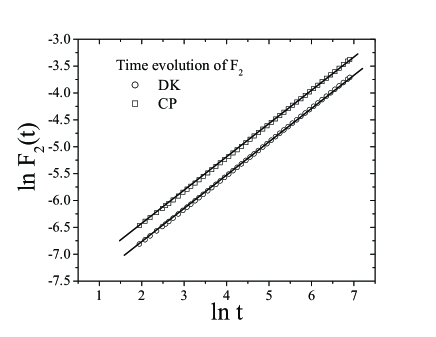
Figure 1: Time evolution of the $F_{2}$ to CP and DK.

To obtain our best estimate, we divide the time interval into subintervals equally spaced in $\ln t$. This avoids placing an undluy large weight on longer times, as would occur if each integer time were treated as a separate data point.

In this case was used $N_{s}=10000$ samples for each independent seed, to a total of 5 seeds, that gives the same $N_{s}=50000$ samples, however with lesser errors due the statistical correlations between samples.

We study various intervals of $\ln t$ to obtain our estimates; for example, for $\ [2.197,6.904]$ we obtain $1/z=0.62867(52)$ and $1/z=0.62802(44)$ respectively for the CP and DK. Our best estimates are found respectively using the intervals $[3.555,6.904]$ for the CP and $[4.9397,6.904]$ for the DK, yielding $1/z=0.63240(25)$ $(z=1.5813(6))$ and $1/z=0.63252(37)$ $(z=$ $1.5810(9))$. These results are more realiable and are consistent with those of Jensen2 and J. R. Mend .

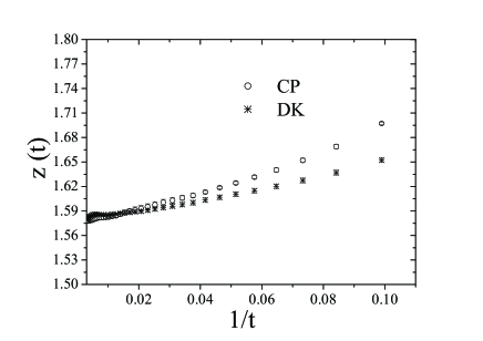
Figure 2: Effective exponent $z(t)$ versus $1/t$ to the CP and DK. Note the convergence to value $z\approx 1.58$ in both cases.

Numerically $z_{t}$ can be estimated from a least-squares linear fit; it is plotted versus $t_{a}^{-1}$, $t_{a}$ being the geometric mean of the $t-$values over the subintervals. The exponents $z_{t}$ and $\nu_{//}$ are similarly obtained, and an extrapolation $t_{a}^{-1}\rightarrow 0$ is performed. In Fig 2 we show this extrapolation for the CP and DK, showing convergence towards $z\approx 1.58$, that reflects the universality between the two models.

The ratio

$$m(t)=\frac{\left\langle\rho^{2}(t)\right\rangle_{\rho_{0}=1}}{\left\langle\rho(t)\right\rangle_{\rho_{0}=1}^{2}}$$ (10)

converges to the expected value for models in the DP universality class, $m_{\infty}\sim 1.1174$ to DP in $(1+1)$ dimensions rdjaff . At short times, $m-1=\mbox{var}(\rho)/\left\langle\rho\right\rangle^{2}$ increases as a power law. The associated exponent is found by noting that

$$\chi\equiv L^{d}\mbox{var}(\rho)\sim t^{\phi}g[(p-p_{c})^{\nu_{||}}t]\overset{t\rightarrow\infty}{\rightarrow}(p-p_{c})^{\gamma}$$ (11)

so that $g(x)\sim x^{-\gamma/\nu_{||}}$ for large $x$. Observing that $\phi=\gamma/\nu_{||}=(d\nu_{\perp}-2\beta)/\nu_{||}$, and that $\left\langle\rho\right\rangle\sim t^{-\beta/\nu_{{}_{||}}}$, we expect $m-1\sim t^{d/z}$. For DP in $(1+1)$ dimensions, $1/z=0.6326$. Our simulations of the CP ($L=5000$, $N_{s}=10000)$, give $z^{-1}=0.634(3)$.

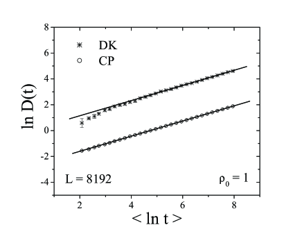
Figure 3: Plot of time evolution of $D(t)$ in the CP and DK.

In the determination of $\nu_{||}$ via Eq. (7), we used $t_{\max}=2980$. In Fig. 3 we show the derivative $D(t)$, and in Fig. 4 the effective exponent $\nu_{||}(t)$ is plotted versus $1/t$ for the CP and DK, for the case $\rho_{0}=1$. We find $\nu_{||}(t)\approx 1.70$, as $t\rightarrow\infty$. We refined this estimate using lattices of $L=2048$, $4096$ and $8192$ for the DK model, to gauge finite-size effects. The estimates for $\nu_{||}$ (using a total of $N_{s}=10000$ realizations, and $\Delta h=2\delta=$ $0.002$) were $1.623(2)$, $1.625(3)$ and $1.648(5)$ respectively.

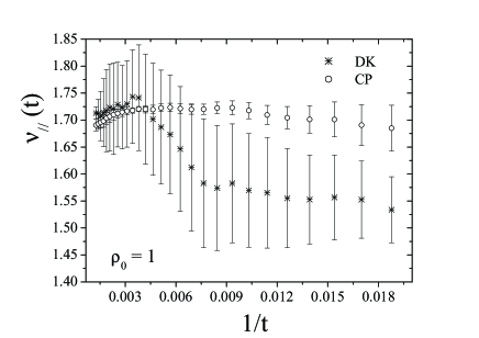
Figure 4: Effective exponent $\nu_{||}(t)$ versus $1/t$ to the CP and DK with $\rho_{0}=1$.

These differ from the accepted value $\nu_{||}=1.733847(6)$ Dickman1 ; Jensen2 . Reducing $\Delta h$ by an order of magnitude, to 0.0002, we obtain $\nu_{||}=1.731(9)$, consistent with the expected result. In the CP simulations we used the reweighting method proposed in Dickman2 . The sample of realizations generated at $\lambda_{c}$ is reweighted for nearby values, $\lambda_{c}\pm n\delta$. Using $\delta=0.001$, we determine $\nu_{||}(t)$ (figure 5) to study the influence of $\Delta h$. The last ten points of each curve are extrapolated to $1/t\rightarrow 0$ to estimate $\nu_{||}$; as $\delta$ is reduced, our estimate approaches the expected value $\nu_{||}\simeq 1.73$. (For $\delta<0.001$ the curves become indistinguishable.) The value found via extrapolation is $\nu_{||}=1.734(8)$, in agreement with the accepted value.

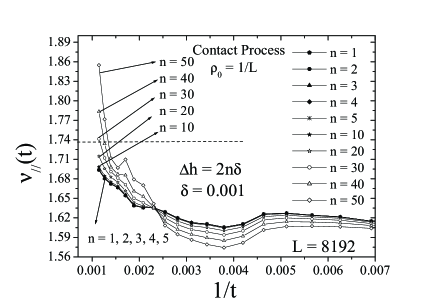
Figure 5: Effects of $\Delta h$ size in the curves of effective exponent in the CP modelo to $\rho_{0}=1/L$. Non-equilibrium reweighting and the continuous time MC method were used.

A interesting way of measure the direct influence of $\Delta h$ in $\nu_{||}$ can be seen in a plot of $\nu_{||}$ as function of $\Delta h$. We note the expected behavior of $\nu_{||}\rightarrow 1.73...$. (figure 6).

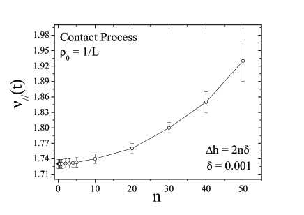
Figure 6: Plot of $\nu_{||}$ as a function of $n$, where $\Delta h=2n\delta$.

IV Summary and Conclusions

We apply several simulation methods based on analysis of short time simulations to determine the critical exponents $z$ and $\nu_{||}$ in models exhibiting a continuous phase transition to an absorbing state. The ratios $F_{2}(t)=\left\langle\rho\right\rangle_{\rho_{0}=1/L^{d}}/\left\langle\rho\right\rangle_{\rho_{0}=1}^{2}$ and $m(t)=\left\langle\rho(t)^{2}\right\rangle_{\rho_{0}=1}/\left\langle\rho(t)\right\rangle_{\rho_{0}=1}^{2}$ have shown to be useful in alternative methods to determine critical exponents of those models. Our estimates for the dynamic critical exponent $z$ ($1.5813(6)$ for the CP and $1.5810(9)$ for the DK cellular automaton) are in good agreement with accepted results in the literature obtained by other techniques such as low-density expansion and exact diagonalization of the master equation.

In order to improve the efficiency in determining the critical exponent $\nu_{||}$ we employ a list of occupied sites and sample reweighting. We also check the influence of $h$, the increment used in evaluating the numerical derivative in Eq. (8). The estimates for $\nu_{||}$ appear to be very sensitive to increment size. Using $\Delta h=2\delta=$ $0.0002$ we obtain our best estimates which are $\nu_{||}=1.731(9)$ for the DK cellular automata and $\nu_{||}=1.734(8)$ for the CP process. These results are in agreement with, though considerably less precise than, the best estimate in the literature, $\nu_{||}=1.733847(6)$ Jensen2 . We believe that the methods investigated here will be useful in the analysis of other models with absorbing states, in particular, in establishing the universality class using short time simulations, which are typically less computationally demanding than studies of the stationary process.

References

- (1) H. Hinrichsen, Adv. Phys, 49, 815 (2000)
- (2) J. Marro, R. Dickman, Nonequilibrium Phase Transitions in Lattice Models, (Cambridge University Press, Cambridge, 1999).
- (3) R. Dickman, Phys. Rev. E 60, R2441 (1999).
- (4) H. K. Janssen, B. Shaub and B. Schmitmann, Z, Phys. B 73, 539 (1989)
- (5) R. da Silva, N. A. Alves, J. R. Drugowich de Felício, Phys. Lett. A 298, 325 (2002)
- (6) R. da Silva, N. A. Alves, J. R. Drugowich de Felício, Phys. Rev. E 66, 026130 (2002);
- (7) T. M. Liggett, ’Interacting Particle Sistems’, Springer-Verlag, New York (1984)
- (8) E. Domany and W. Kinzel, Phys. Rev. Lett, 53, 311 (1984)
- (9) J. W. Essam, J. Phys. A: Math. Gen. 22, 4927 (1989).
- (10) I. Jensen, J. Phys. A, 32, 5233 (1999)
- (11) P. Grassberger, Y. Zhang, Physica A 224, 169 (1996)
- (12) J. R. G. de Mendonça, J. Phys. A, 32, L467 (1999)
- (13) R. Dickman and J. Kamphorst Leal da Silva, Phys Rev. E58, 4266 (1998).