Pumped spin-current and shot noise spectra in a single quantum dot

Abstract

We exploit the pumped spin-current and current noise spectra under equilibrium condition in a single quantum dot connected to two normal leads, as an electrical scheme for detection of the electron spin resonance (ESR) and decoherence. We propose spin-resolved quantum rate equations with correlation functions in Laplace-space for the analytical derivation of the zero-frequency atuo- and cross-shot noise spectra of charge- and spin-current. Our results show that in the strong Coulomb blockade regime, ESR-induced spin flip generates a finite spin-current and the quantum partition noises in the absence of net charge transport. Moreover, spin shot noise is closely related to the magnetic Rabi frequency and decoherence and would be a sensitive tool to measure them.

Introduction—There have been extensive investigations focused on electron spin detection and measurement via charge transport in mesoscopic quantum dot (QD) system,Engel ; Balatsky ; Martin which is motivated from the fact that easy preparation and manipulation of electron spins, as well as the remarkably long spin coherence time, provide the way for applications in spintronics and quantum information processing.Prinz In these systems, transport is governed not only by the charge flow, but also by the spin dynamics. Recently, a pure spin current has been reported by direct optical injection without generation of a net charge current.Stevens Theoretically, a spin source device has also been proposed to carry pure spin flow based on electron spin resonance (ESR) in a QD-lead system with sizable Zeeman splitting.Wang1 ; Zhang Moreover, both auto- and cross-correlation noise spectra of spin-current have been studied for this QD-based spin battery.Wang2

However, Coulomb blockade (CB) effect on this QD spin battery needs investigation, since CB effect is an essential feature of transport through a QD. More importantly, the spin configuration of the confined electrons on QD is apparently affected by CB effect, which directly determine the efficiency of this device. As well, these previous studies also neglected the inevitable spin decoherence due to coupling of the single spin with environment. Therefore, it is the purpose of this paper to study this ERS-pumped spin-current and its fluctuations for a QD connected with two normal leads in the strong CB regime at zero temperature. The setup is schematically depicted in Fig. 1: The single electron levels in the dot are split by an external magnetic field $B$, $\epsilon_{\downarrow}-\epsilon_{\uparrow}=g_{z}\mu_{B}B$ ($=\Delta$ Zeeman energy), where $g_{z}$ is the effective electron g-factor in the $z$ direction and $\mu_{B}$ is the Bohr magneton. The gate voltage controls the chemical potentials $\mu$ of two leads located between the two split levels and no bias voltage is applied to the two leads. After a spin-up electron tunnels into the QD, an oscillating magnetic field $B_{\rm rf}(t)=(B_{\rm rf}\cos\Omega t,\,B_{\rm rf}\sin\Omega t$) applied perpendicularly to the constant field $B$ with the frequency $\Omega$ nearly equal to $\Delta$ can pump electron to the higher level where its spin is flipped, then the spin-down electron can tunnel out to the leads. Because the two currents with opposite directions have different spin orientations, spin-currents are established in both leads with equal values. If the Coulomb interaction in the QD is strong enough to prohibit the double occupation, no more electrons can enter the QD before the spin-down electron exits. As a result, the number of electrons exiting from the QD is equal to that of electrons entering the QD, namely, the charge currents exactly cancel out each other. Otherwise, in the case $\epsilon_{\uparrow}+U<\mu$ the ESR pumping will generate both spin-current and charge-current. Note that both leads have contributions to the spin-current of one lead, causing the correlation of spin-currents in different leads, which provides possibility of studying cross-correlation of spin currents without bias voltage.Sauret

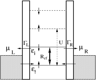
Figure 1: Schematic view for the QD-based spin battery.

Theoretical formalism—We write the Hamiltonian of the ESR-induced spin battery under consideration as:

$$H = \sum_{\eta,k,\sigma}\epsilon_{\eta k\sigma}c_{\eta k\sigma}^{\dagger}c_{\eta k\sigma}^{{\phantom{\dagger}}}+\sum_{\sigma}\epsilon_{\sigma}c_{d\sigma}^{\dagger}c_{d\sigma}^{{\phantom{\dagger}}}+Un_{d\uparrow}n_{d\downarrow}$$ (2)

$$+\sum_{\eta,k,\sigma}(V_{\eta}c_{\eta k\sigma}^{\dagger}c_{d\sigma}^{{\phantom{\dagger}}}+{\rm{H.c.}})+H_{\rm rf}(t),$$

where $c_{\eta k\sigma}^{\dagger}$ ($c_{\eta k\sigma}$) and $c_{d\sigma}^{\dagger}$ ($c_{d\sigma}$) are the creation (annihilation) operators for electrons with momentum $k$, spin-$\sigma$ and energy $\epsilon_{\eta k\sigma}$ in the lead $\eta$ ($={\rm L,R}$) and for a spin-$\sigma$ electron on the QD, respectively. The third term describes the Coulomb interaction among electrons on the QD. $n_{d\sigma}=c_{d\sigma}^{\dagger}c_{d\sigma}^{{\phantom{\dagger}}}$ is the occupation operator in the QD. The fourth term represents the tunneling coupling between the QD and the reservoirs. The last term $H_{\rm rf}(t)$ describes the coupling between the spin states due to the rotating field $B_{\rm rf}(t)$ and can be written, in the rotating wave approximation (RWA), as

$$H_{\rm rf}(t)=R_{\rm rf}\big{(}c_{d\uparrow}^{\dagger}c_{d\downarrow}^{{\phantom{\dagger}}}e^{i\Omega t}+c_{d\downarrow}^{\dagger}c_{d\uparrow}^{{\phantom{\dagger}}}e^{-i\Omega t}\big{)},$$ (3)

with the ESR Rabi frequency $R_{\rm rf}=g_{\perp}\mu_{B}B_{\rm rf}/2$, with the g-factor $g_{\perp}$ and the amplitude of the rf field $B_{\rm rf}$.

Here, in order to anticipate the CB and the intrinsic spin relaxation, we utilize the quantum rate equations for the system density matrix elements: $\rho_{00}$ and $\rho_{\sigma\sigma}$ describe the occupation probability in the QD being, respectively, unoccupied and spin-$\sigma$ states, and the off-diagonal term $\rho_{\uparrow\downarrow(\downarrow\uparrow)}$ denotes coherent superposition of the two coupled spin states in the QD.Gurvitz The doubly-occupied state is prohibited due to the infinite Coulomb interaction $U\rightarrow\infty$. Here we focus our interest on the nonadiabatic pumping where the photo-assisted resonance is achieved and neglect cotunneling processes. For the purpose of evaluating the noise spectrum, we introduce the spin-resolved (in both terminals) density matrices $\rho_{ab}^{({m_{L\uparrow},m_{R\uparrow}\atop m_{L\downarrow},m_{R\downarrow}})}(t)$, meaning that the QD is on the electronic state $|a\rangle$ ($a=b=0,\,\uparrow,\,\downarrow$) or on quantum superposition state ($a\neq b$) at time $t$ together with $m_{L\uparrow}$ ($m_{R\uparrow}$) spin-up electrons and $m_{L\downarrow}$ ($m_{R\downarrow}$) spin-down electrons in the left (right) lead. Obviously, $\rho_{ab}(t)=\sum_{m_{L\uparrow},m_{R\uparrow}\atop m_{L\downarrow},m_{R\downarrow}}\rho_{ab}^{({m_{L\uparrow},m_{R\uparrow}\atop m_{L\downarrow},m_{R\downarrow}})}(t)$ and the quantum rate equations for these spin-resolved density matrices in the rotating frame with respect to $\Omega$ are

$$\dot{\rho}_{00}^{({m_{L\uparrow},m_{R\uparrow}\atop m_{L\downarrow},m_{R\downarrow}})} = \Gamma_{L\downarrow}\rho_{\downarrow\downarrow}^{({m_{L\uparrow},m_{R\uparrow}\atop m_{L\downarrow}-1,m_{R\downarrow}})}+\Gamma_{R\downarrow}\rho_{\downarrow\downarrow}^{({m_{L\uparrow},m_{R\uparrow}\atop m_{L\downarrow},m_{R\downarrow}-1})}$$ (4b)

$$-(\Gamma_{L\uparrow}+\Gamma_{R\uparrow})\rho_{00}^{({m_{L\uparrow},m_{R\uparrow}\atop m_{L\downarrow},m_{R\downarrow}})},$$

$$\dot{\rho}_{\uparrow\uparrow}^{({m_{L\uparrow},m_{R\uparrow}\atop m_{L\downarrow},m_{R\downarrow}})} = \Gamma_{L\uparrow}\rho_{00}^{({m_{L\uparrow}+1,m_{R\uparrow}\atop m_{L\downarrow},m_{R\downarrow}})}+\Gamma_{R\uparrow}\rho_{00}^{({m_{L\uparrow},m_{R\uparrow}+1\atop m_{L\downarrow},m_{R\downarrow}})}$$ (4e)

$$+\frac{1}{2T_{1}}\rho_{\downarrow\downarrow}^{({m_{L\uparrow},m_{R\uparrow}\atop m_{L\downarrow},m_{R\downarrow}})}-\frac{1}{2T_{1}}\rho_{\uparrow\uparrow}^{({m_{L\uparrow},m_{R\uparrow}\atop m_{L\downarrow},m_{R\downarrow}})}$$

$$+iR_{\rm rf}(\rho_{\uparrow\downarrow}^{({m_{L\uparrow},m_{R\uparrow}\atop m_{L\downarrow},m_{R\downarrow}})}-\rho_{\downarrow\uparrow}^{({m_{L\uparrow},m_{R\uparrow}\atop m_{L\downarrow},m_{R\downarrow}})}),$$

$$\dot{\rho}_{\downarrow\downarrow}^{({m_{L\uparrow},m_{R\uparrow}\atop m_{L\downarrow},m_{R\downarrow}})} = -(\Gamma_{L\downarrow}+\Gamma_{R\downarrow})\rho_{\downarrow\downarrow}^{({m_{L\uparrow},m_{R\uparrow}\atop m_{L\downarrow},m_{R\downarrow}})}+\frac{1}{2T_{1}}\rho_{\uparrow\uparrow}^{({m_{L\uparrow},m_{R\uparrow}\atop m_{L\downarrow},m_{R\downarrow}})}$$ (4g)

$$-\frac{1}{2T_{1}}\rho_{\downarrow\downarrow}^{({m_{L\uparrow},m_{R\uparrow}\atop m_{L\downarrow},m_{R\downarrow}})}+iR_{\rm rf}(\rho_{\uparrow\downarrow}^{({m_{L\uparrow},m_{R\uparrow}\atop m_{L\downarrow},m_{R\downarrow}})}-\rho_{\downarrow\uparrow}^{({m_{L\uparrow},m_{R\uparrow}\atop m_{L\downarrow},m_{R\downarrow}})}),$$

$$\dot{\rho}_{\uparrow\downarrow}^{({m_{L\uparrow},m_{R\uparrow}\atop m_{L\downarrow},m_{R\downarrow}})} = iR_{\rm rf}(\rho_{\uparrow\uparrow}^{({m_{L\uparrow},m_{R\uparrow}\atop m_{L\downarrow},m_{R\downarrow}})}-\rho_{\downarrow\downarrow}^{({m_{L\uparrow},m_{R\uparrow}\atop m_{L\downarrow},m_{R\downarrow}})})$$ (4i)

$$+i\delta_{\rm ESR}\rho_{\uparrow\downarrow}^{({m_{L\uparrow},m_{R\uparrow}\atop m_{L\downarrow},m_{R\downarrow}})}-[\frac{1}{2}(\Gamma_{L\downarrow}+\Gamma_{R\downarrow})+\frac{1}{T_{2}}]\rho_{\uparrow\downarrow}^{({m_{L\uparrow},m_{R\uparrow}\atop m_{L\downarrow},m_{R\downarrow}})},$$

and the normalization relation $\rho_{00}+\sum_{\sigma}\rho_{\sigma\sigma}=1$. The equation of motion for $\rho_{\downarrow\uparrow}^{({m_{L\uparrow},m_{R\uparrow}\atop m_{L\downarrow},m_{R\downarrow}})}$ can be obtained by implementing complex conjugate on Eq. (4i). In these equations, $\delta_{\rm ESR}=\Delta-\Omega$ is the ESR detuning and $\Gamma_{\eta\sigma}=2\pi\sum_{k}|V_{\eta}|^{2}\delta(\omega-\epsilon_{\eta k\sigma})$ denotes the strength of coupling between the QD and the lead $\eta$ involving spin $\sigma$. In wide band limit, these tunneling amplitudes are independent of energy and for simplicity we set $\Gamma_{\eta\uparrow}=\Gamma_{\eta\downarrow}=\Gamma/2$. Furthermore, we describe the coupling of single spin with the environment in a phenomenological way via introducing two time scales: the spin relaxation time $T_{1}$ of an excited spin state into the thermal equilibrium, and the spin decoherence time $T_{2}$ related to the loss of phase coherence of the spin superposition state. The measurement of $T_{2}$ in QDs is currently active topic because it is the limit time scale for coherent spin manipulation and thus quantum information processing. In typical GaAs QD, $\Gamma=8~{}\mu$eV, corresponding to a tunneling time $\tau\sim\Gamma^{-1}=0.5$ ns. To observe single- and multi-photon effects in tunneling (nonadiabatic regime), it must require the spin flipping time $T_{\Omega}<\tau$. If one takes $B=1~{}$T, the Zeeman energy is $\Delta=26~{}\mu$eV which determine the optimal driving frequency $\Omega=13\pi~{}$GHz and the corresponding $T_{\Omega}=0.15~{}$ns. These proposed spin-device parameters can be easily realized by present technology.

Recently, $T_{1}$ in a single QD was probed to be an order of microsecond via transport experiment,Fujisawa which is notably longer than other time scales $T_{1}\gg T_{2},\,\tau,\,T_{\Omega}$. Hence it is a good approximation to assume $T_{1}\rightarrow\infty$ in the following calculation. Consequently, one recovers the usual quantum rate equations for the reduced density matrix elements $\rho_{ab}(t)$ for a single QD with spin coupling: $\dot{\bm{\rho}}(t)=(\dot{\rho}_{00},\dot{\rho}_{\uparrow\uparrow},\dot{\rho}_{\downarrow\downarrow},\dot{\rho}_{\uparrow\downarrow},\dot{\rho}_{\downarrow\uparrow})={\cal M}{\bm{\rho}}(t)$ withMartin ; Gurvitz

$${\cal M}=\left(\begin{array}[]{ccccc}-\Gamma_{\uparrow}&0&\Gamma_{\downarrow}&0&0\\ \Gamma_{\uparrow}&0&0&iR_{\rm rf}&-iR_{\rm rf}\\ 0&0&-\Gamma_{\downarrow}&-iR_{\rm rf}&iR_{\rm rf}\\ 0&iR_{\rm rf}&-iR_{\rm rf}&-\Gamma_{\downarrow}V+i\delta_{\rm ESR}&0\\ 0&-iR_{\rm rf}&iR_{\rm rf}&0&-\Gamma_{\downarrow}V+i\delta_{\rm ESR}\end{array}\right),$$ (5)

and $V=\frac{1}{2}+\frac{1}{\Gamma_{\downarrow}T_{2}}$.

Spin-current—The spin-related currents $I_{\eta\sigma}$ can be evaluated by the time change rate of spin-$\sigma$ electron number in the $\eta$ lead

$$I_{\eta\sigma} = e\dot{N}_{\eta\sigma}=e\frac{d}{dt}\sum_{m_{L\uparrow},m_{R\uparrow}\atop m_{L\downarrow},m_{R\downarrow}}m_{\eta\sigma}P(t){\big{|}}_{t\rightarrow\infty},$$ (6)

$$P(t) = \rho_{00}^{({m_{L\uparrow},m_{R\uparrow}\atop m_{L\downarrow},m_{R\downarrow}})}(t)+\rho_{\uparrow\uparrow}^{({m_{L\uparrow},m_{R\uparrow}\atop m_{L\downarrow},m_{R\downarrow}})}(t)+\rho_{\downarrow\downarrow}^{({m_{L\uparrow},m_{R\uparrow}\atop m_{L\downarrow},m_{R\downarrow}})}(t).$$

In particular, using Eqs. (4) we find $I_{L\uparrow}=-e\Gamma_{L\uparrow}\rho_{00}$ and $I_{L\downarrow}=e\Gamma_{L\downarrow}\rho_{\downarrow\downarrow}$. The stationary solution of Eqs. (4) is:

$$\rho_{\uparrow\uparrow} = \frac{2R_{\rm rf}^{2}V+\delta_{\rm ESR}^{2}+\Gamma^{2}V^{2}}{\Xi},$$ (7)

$$\rho_{\downarrow\downarrow} = \frac{2R_{\rm rf}^{2}V}{\Xi},$$ (8)

$$\rho_{\uparrow\downarrow} = \frac{R_{\rm rf}[i\Gamma V-\delta_{\rm ESR}]}{\Xi},$$ (9)

with $\Xi=6R_{\rm rf}^{2}V+\Gamma^{2}V^{2}+\delta_{\rm ESR}^{2}$. Obviously, the stationary charge-current is exactly zero $I_{\eta}^{c}=I_{\eta\uparrow}+I_{\eta\downarrow}=0$, while the spin-current is

$$I_{L}^{s}=I_{L\downarrow}-I_{L\uparrow}=e\frac{2R_{\rm rf}^{2}\Gamma V}{\Xi},\,\,\,\,I_{R}^{s}=-I_{L}^{s}.$$ (10)

Explicitly, the spin-current is proportional to the excitation power, which is consistent with the prototype of this ESR-based spin battery. And it’s amplitude exhibits a saturation behavior with increasing driving field as a consequence of the nonlinear photon-absorption of a single spin [Fig. 2(a)]. The saturated value is $e\Gamma/3$ independent on the decoherence time $T_{2}$ and detuning $\delta_{\rm ESR}$. Figure 2(b) shows that the detailed dependence of the spin-current on the driving frequency is determined by the spin decoherence time $T_{2}$. In the inset of Fig. 2(a), we show that nonzero charge-current is also pumped by the driving field unless the double occupation is prohibited owing to the strong charging effect $\Gamma^{\prime}=0$.U This verifies our statement in the introduction.

Figure 2: The spin-current vs (a) strength and (b) detuning of the driving field for different spin decoherence time. Inset in (a): Overview of the charge- and spin-current with the Coulomb correlation $\Gamma^{\prime}$. The calculated strength of the oscillation magnetic field corresponds to $0\sim 1~{}$T.

Spin shot noise—Recently nonequilibrium quantum shot noise is another current active subject in mesoscopic physics, because the current correlation (CC) is inherently related to the quantization of electron charge and thus give unique information about electronic correlation, which cannot be obtained by probing the conductance only.Blanter For instance, the cross-correlation for charge-current (the correlation between different terminals) is negative for a normal single-electron transistor, meaning anti-bunching of the wavepacket. Interestingly, much studies have been devoted to find a system where the cross-correlation changes its sign.Samuelsson Here we would like to address that the spin-resolved CC is more useful to describe electron correlation, because the electronic wavepacket with opposite spins is uninfluenced by the Pauli exclusion principle and only reflects unambiguous information about the interaction. For the purpose of evaluating the charge and spin CC from the quantum rate equations (4), we extend the MacDonald’s formula for the spin-resolved situation:MacDonald

$$S_{\eta\eta^{\prime}}^{\sigma\sigma^{\prime}}(\omega) = 2\omega e^{2}\int_{0}^{\infty}dt\sin(\omega t)\frac{d}{dt}{\Big{\{}}\sum_{m_{L\uparrow},m_{R\uparrow}\atop m_{L\downarrow},m_{R\downarrow}}m_{\eta\sigma}m_{\eta^{\prime}\sigma^{\prime}}$$ (12)

$$\times P(t)-t^{2}I_{\eta\sigma}I_{\eta^{\prime}\sigma^{\prime}}/e^{2}{\Big{\}}}.$$

Specially, the zero-frequency shot noise spectrum is

$$S_{\eta\eta^{\prime}}^{\sigma\sigma^{\prime}}(0)=2e^{2}\frac{d}{dt}{\Big{\{}}\sum_{m_{L\uparrow},m_{R\uparrow}\atop m_{L\downarrow},m_{R\downarrow}}m_{\eta\sigma}m_{\eta^{\prime}\sigma^{\prime}}P(t)-\frac{t^{2}}{e^{2}}I_{\eta\sigma}I_{\eta^{\prime}\sigma^{\prime}}{\Big{\}}}{\big{|}}_{t\rightarrow\infty}.$$ (13)

The auto- and cross-noise spectra of the charge-current and spin-current can be obtained from these correlations $S_{\eta\eta^{\prime}}^{\sigma\sigma^{\prime}}$: $S_{\eta\eta^{\prime}}^{c/s}=S_{\eta\eta^{\prime}}^{\uparrow\uparrow}+S_{\eta\eta^{\prime}}^{\downarrow\downarrow}\pm S_{\eta\eta^{\prime}}^{\uparrow\downarrow}\pm S_{\eta\eta^{\prime}}^{\downarrow\uparrow}$.

In order to evaluate these correlations, we introduce the following generating functions:

$$G_{\eta\sigma}^{ab}(t)=\sum_{m_{L\uparrow},m_{R\uparrow}\atop m_{L\downarrow},m_{R\downarrow}}m_{\eta\sigma}\rho_{ab}^{({m_{L\uparrow},m_{R\uparrow}\atop m_{L\downarrow},m_{R\downarrow}})}(t).$$ (14)

With the help of Eqs. (4), all noise spectra are therefore relevant with these auxiliary functions and $\rho_{ab}(t)$ as:

$$\frac{S_{\eta\eta^{\prime}}^{\sigma\sigma^{\prime}}(0)}{2e^{2}} = {\big{\{}}\frac{1}{2}\Gamma_{\sigma}\delta_{\sigma\sigma^{\prime}}[\delta_{\eta\eta^{\prime}}(\rho_{00}(t)\delta_{\sigma\uparrow}+\rho_{\downarrow\downarrow}(t)\delta_{\sigma\downarrow})$$ (17)

$$+\sum_{\eta^{\prime\prime}}(G_{\eta^{\prime\prime}\sigma}^{\downarrow\downarrow}(t)\delta_{\sigma\downarrow}-G_{\eta^{\prime\prime}\sigma}^{00}(t)\delta_{\sigma\uparrow})]+\delta_{\sigma\bar{\sigma^{\prime}}}[\frac{1}{2}\Gamma_{\downarrow}G_{\eta\uparrow}^{\downarrow\downarrow}(t)$$

$$-\frac{1}{2}\Gamma_{\uparrow}G_{\eta^{\prime}\downarrow}^{00}(t)]-\frac{2t}{e^{2}}I_{\eta\sigma}I_{\eta^{\prime}\sigma^{\prime}}{\big{\}}}{\big{|}}_{t\rightarrow\infty}.$$

On the other hand, using Eqs.(4), the equations of motion for ${\bf G}_{\eta\sigma}(t)$ is explicitly obtained in matrix form: $\dot{\bf G}_{\eta\sigma}(t)={\cal M}{\bf G}_{\eta\sigma}(t)+{\cal G}_{\eta\sigma}{\bm{\rho}}(t)$ with

$${\cal G}_{\eta\sigma}=\left(\begin{array}[]{ccccc}0&0&\Gamma_{\eta\downarrow}\delta_{\sigma\downarrow}&0&0\\ -\Gamma_{\eta\uparrow}\delta_{\sigma\uparrow}&0&0&0&0\\ 0&0&0&0&0\\ 0&0&0&0&0\\ 0&0&0&0&0\end{array}\right).$$ (18)

Applying Laplace transform to these equations yields

$${\bf G}_{\eta\sigma}(s)=(s{\bf I}-{\cal M})^{-1}{\cal G}_{\eta\sigma}{\bm{\rho}}(s),$$ (19)

where ${\bm{\rho}}(s)$ is readily obtained by performing Laplace transform on its equations of motion and the normalization relation. Due to inherent long-time stability of the physics system under investigation, all real parts of nonzero poles of ${\bm{\rho}}(s)$ and ${\bf G}(s)$ are negative definite. Consequently, the large-$t$ behavior of the auxiliary functions is entirely determined by the divergent terms of the partial fraction expansions of ${\bm{\rho}}(s)$ and ${\bf G}_{\eta\sigma}(s)$ at $s\rightarrow 0$.

Resolving both ${\bf G}_{\eta\sigma}(s)$ and ${\bm{\rho}}(s)$ into the partial fraction expansion forms and performing inverse Laplace transform, we can eventually derive the analytical expressions for these large-$t$ asymptotic correlations. Surprisingly, we find the zero-frequency charge shot noises being proportional to the spin-current $S_{LL}^{c}=-S_{LR}^{c}=e^{2}|I_{L}^{s}|$, which manifests that pumping processes do generate shot noise even in the absence of net charge-current. This feature is underlying analog of the quantum partition noise of photo-excited electron-hole pairs demonstrated in the recent experiment.Reydellet Spin-up and spin-down electrons in this spin battery are dissociated by tunneling events in the presence of pumping field but without bias: spin-up electrons inject into the QD, but spin-down electrons flow off in an opposite direction. As expected, the cross-correlation of the charge noise is always negative definite, showing anti-bunching statistics, but it has the same magnitude with the auto-correlation of the charge-current originated from the conservation law of charge.Wang2

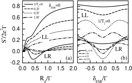
Figure 3: The zero-frequency auto- and cross-correlations of spin-current vs (a) strength and (b) detuning of driving field.

However, the situation is very different for the zero-frequency spin shot noise, as shown in Fig. 3. The auto-correlation of the spin-current is surely positive definite, while the cross-correlation is either positive or negative depending on a number of parameters: the pumping amplitude $R_{\rm rf}$, the detuning $\delta_{\rm ESR}$, and the decoherence $T_{2}$. For small decoherence rates, the spin cross-correlation experiences the change of sign with increasing excitation $R_{\rm rf}$ at resonant pumping $\delta_{\rm ESR}=0$. Interestingly, this cross-correlation is always positive (1) at large excitation $R_{\rm rf}>\Gamma$ regardless of decoherence $T_{2}$ [Fig. 3(a)] or (2) if apart away from quantum resonance [Fig. 3(b)]. The significant role of decoherence is to evidently reduce these noise spectra and even to eliminate the change of sign in the spin cross-correlation. It is addressed that spin shot noise is more sensitive to the spin decoherence than the spin-current and the charge shot noise. This could provide a way to measure the spin decoherence time $T_{2}$.

In summary, we have presented a generic method for analytical calculation of the atuo- and cross-shot noise spectra of charge- and spin-current in an ESR-based single QD system. We found that in the strong CB regime, indeed ESR pumping generates a finite spin-current and quantum partition noises in the absence of net charge transport. And the spin shot noises display complicated behaviors depending on the pumping parameters and the spin decoherence time. The measurement of spin-current and shot noise provides a scheme for the Rabi oscillation and spin decoherence detections in the QD system.

BD and HLC are supported by the DURINT Program administered by the US Army Research Office. XLL is supported by Major Projects of National Natural Science Foundation of China, the Special Founds for Major State Basic Research Project and the Shanghai Municipal Commission of Science and Technology.

References

• (1) H.A. Engel and D. Loss, Phys. Rev. Lett. 86, 4648 (2001); Phys. Rev. B 65, 195321 (2002).
• (2) A.V. Balatsky and I. Martin, cond-mat/0112407; D. Mozyrsky, L. Fedichkin, S.A. Gurvitz, and G.P. Berman, Phys. Rev. B 66, 161313 (2002); J.X. Zhu and A.V. Balatsky, Phys. Rev. Lett. 89, 286802 (2002).
• (3) I. Martin, D. Mozyrsky, and H.W. Jiang, Phys. Rev. Lett. 90, 18301 (2003).
• (4) G.A. Prinz, Science 282, 1660 (1998); S.A. Wolf, D.D. Awschalom, R.A. Buhrman, J.M. Daughton, S.V. Molnar, M.L. Roukes, A.Y. Chtchelkanova, D.M. Treger, Science 294, 1488 (2001).
• (5) M.J. Stevens, A.L. Smirl, R.D.R. Bhat, A. Najmaie, J.E. Sipe, and H.M. van Driel, Phys. Rev. Lett. 90, 136603 (2003); J. HΓΌbner, W.W. RΓΌhle, M. Klude, D. Hommel, R.D.R. Bhat, J.E. Sipe, and H.M. van Driel, Phys. Rev. Lett. 90, 216601 (2003).
• (6) B.G. Wang, J. Wang, and H. Guo, Phys. Rev. B 67, 92408 (2003).
• (7) P. Zhang, Q.K. Xue, and X.C. Xie, Phys. Rev. Lett. 91, 196602 (2003).
• (8) B.G. Wang, J. Wang, and H. Guo, cond-mat/0305066 (2003).
• (9) O. Sauret and D. Feinberg, Phys. Rev. Lett. 92, 106601 (2004).
• (10) S.A. Gurvitz and Ya.S. Prager, Phys. Rev. B 53, 15932 (1996); B. Dong, H.L. Cui, and X.L. Lei, Phys. Rev. B 69 35324 (2004).
• (11) T. Fujisawa, Y. Tokura, and Y. Hirayama, Phys. Rev. B 63 81304(R) (2001).
• (12) Extension of zero-temperature spin-resolved quantum rate equations and current formula are easily achieved for considering the doubly occupied state. See Ref.Β Gurvitz, . Charging effect is modeled by tunneling rate $\Gamma^{\prime}$.
• (13) Ya.M. Blanter and M. BΓΌttiker, Phys. Rep. 336, 1 (2000).
• (14) P. Samuelsson and M. BΓΌttiker, Phys. Rev. Lett. 89, 46601 (2002); F. Taddei and R. Fazio, Phys. Rev. B 65, 134522 (2002); D. SΓ‘nchez, R. LΓ³pez, P. Samuelsson, and M. BΓΌttiker, Phys. Rev. B 68, 214501 (2003).
• (15) D.K.C. MacDonald, Rep. Prog. Phys. 12, 56 (1948); L.Y. Chen and C.S. Ting, Phys. Rev. B 46, 4714 (1992).
• (16) L.H. Reydellet, P. Roche, D.C. Glattli, B. Etienne, and Y. Jin, Phys. Rev. Lett. 90, 176803 (2003).