Stability of $\pi$ junction configurations in ferromagnet-superconductor heterostructures

Abstract

We investigate the stability of possible order parameter configurations in clean layered heterostructures of the $SFS...FS$ type, where $S$ is a superconductor and $F$ a ferromagnet. We find that for most reasonable values of the geometric parameters (layer thicknesses and number) and of the material parameters (such as magnetic polarization, wavevector mismatch, and oxide barrier strength) several solutions of the self consistent microscopic equations can coexist, which differ in the arrangement of the sequence of “0” and “$\pi$” junction types (that is, with either same or opposite sign of the pair potential in adjacent $S$ layers). The number of such coexisting self consistent solutions increases with the number of layers. Studying the relative stability of these configurations requires an accurate computation of the small difference in the condensation free energies of these inhomogeneous systems. We perform these calculations, starting with numerical self consistent solutions of the Bogoliubov-de Gennes equations. We present extensive results for the condensation free energies of the different possible configurations, obtained by using efficient and accurate numerical methods, and discuss their relative stabilities. Results for the experimentally measurable density of states are also given for different configurations and clear differences in the spectra are revealed. Comprehensive and systematic results as a function of the relevant parameters for systems consisting of three and seven layers (one or three junctions) are given, and the generalization to larger number of layers is discussed.

I Introduction

A remarkable manifestation of the macroscopic quantum nature of superconductivity is seen in the description of the superconducting state by a complex order parameter with an associated phase, $\phi$, which is a macroscopic quantum variable. For composite materials comprised of multiple superconductor ($S$) layers separated by nonsuperconducting materials, the phase difference $\Delta\phi$ between adjacent $S$ layers becomes a very relevant quantity. For the case where a nonmagnetic normal metal is sandwiched between two superconductors, it is straightforward to see that the minimum free energy configuration corresponds to that having a zero phase difference between the $S$ regions, in the absence of current. The situation becomes substantially modified for superconductor-ferromagnet-superconductor ($SFS$) junctions, where the presence of the magnetic ($F$) layers leads to spin-split Andreevand states and to a spatially modulatedff ; lo order parameter that can yield a phase difference of $\Delta\phi=\pi$ between $S$ layers. These are the so-called $\pi$ junctions. Junctions of this type can occur also in more complicated layered heterostructures of the $SFSFSF..$ type, where the relative sign of the pair potential $\Delta({\bf r})$ can change between adjacent $S$ layers.

Continual improvements in well controlled deposition and fabrication techniques have helped increase the experimental implementations of systems containing $\pi$ junctions. vavra ; bell ; jiang ; lange ; kontos ; kontos2 ; ryazanov ; veret ; frolov ; goldobin Possible applications to devices and to quantum computing, as well as purely scientific interest, have stimulated further interest in these devices. The pursuit of the $\pi$ state has consequently generated ample supporting data for its existence and properties: The observed nonmonotonic behavior in the critical temperature was found to be consistent with the existence of a $\pi$ state.jiang The domain structure in $F$ is expected to modify the critical temperature behavior however, depending on the applied field.lange The ground state of $SFS$ junctions has been recently measured,kontos and it was found that $0$ or $\pi$ coupling existed, depending on the width $d_{F}$ of the $F$ layer, in agreement with theoretical expectations. Similarly, damped oscillations in the critical current $I_{C}$ as a function of $d_{F}$ suggested also a $0$ to $\pi$ transition.kontos2 The reported signature in the characteristic $I_{C}$ curves also indicated a crossover from the $0$ to $\pi$ phase in going from higher to lower temperatures.ryazanov Furthermore, the current phase relation was measured,frolov demonstrating a re-entrant $I_{C}$ with temperature variation.

A good understanding of the mechanism and robustness of the $\pi$ state in general is imperative for the further scientific and practical development of this area. The $\pi$ state in $SFS$ structures was first investigated long ago.bulaevskii In general, the exchange field in the ferromagnet shifts the different spin bands occupied by the corresponding particle and hole quasiparticles. This splitting determines the spatial periodicity of the pair amplitude in the $F$ layerdab and can therefore induce a crossover from the $0$ state to the $\pi$ state as the exchange field $h_{0}$ varies,buzdin or as a function of $d_{F}$. The Josephson critical current was found to be nonzero at the $0$ to $\pi$ transition, as a result from higher harmonics in the current-phase relationship.belzig It was found that a coexistence of stable and metastable states may arise in Josephson junctions, which was also attributed to the existence of higher harmonics.radovic If the magnetization orientation is varied, the $\pi$ state may disappear,bergeret in conjunction with the appearance of a triplet component to the order parameter. A crossover between $0$ and $\pi$ states by varying the temperature was explained within the context of a Andreev bound state model that reproduced experimental findings.sellier In the ballistic limit a transition occurs if the parameters of the junction are close to the crossover at zero temperature.radovic2 An investigation into the ground states of long (but finite) Josephson junctions revealed a critical geometrical length scale which separates half-integer and zero flux states.zenchuk The lengths of the individual junctions were also found to have important implications, as a phase modulated state can occur through a second order phase transition.buzdin2

Nevertheless, little work has been done that studies the stability of the $\pi$ state for an $SFS$ junction from a complete and systematic standpoint, as a function of the relevant parameters. This is a fortiori true for layered systems involving more than one junction, each of which can in principle exist in the 0 or the $\pi$ state, or for superlattices. There are several reasons for this. The existence or absence of $\pi$ junction states is intimately connected to the spatial behavior of $\Delta({\bf r})$ and of the pair amplitude $F({\bf r})$ (which oscillates in the magnetic layers), and thus the precise form of these quantities must be calculated self-consistently, so that the resulting $F({\bf r})$ corresponds to a minimum in the free energy. An assumed, non self consistent form for the pair potential, typically a piecewise constant in the $S$ layers, often deviates very substantially from the correct self consistent result, and therefore may often lead to spurious conclusions. Indeed, the assumed form may in effect force the form of the final result, thereby clearly leading to misleading results. Self-consistent approaches, despite their obvious superiority, are too infrequently found in the literature primarily because of the computational expense inherent in the variational or iterative methods necessary to achieve a solution. A second problem is that investigation the relative stability of self-consistent states requires an accurate calculation of their respective condensation energies, and that, too, is not an easy problem.

In this paper, we approach in a fully self consistent manner the question of the stability of states containing $\pi$ junctions in $SFSF...S$ multilayer structures. As has already been shown in trilayers,hv3 it can be the case that, for a given set of geometrical and material parameters, more than one self consistent solution exists, each with a particular spatial profile for $\Delta({\bf r})$ involving a junction of either the 0 or $\pi$ type. It will be demonstrated below that this is in fact a very common situation in these heterostructures: one can typically find several solutions, all with a negative condensation energy, i.e., they are all stable with respect to the normal state. Thus a careful analysis is needed to determine whether each state is a global or local minimum of the condensation free energy. This determination is, as we shall see, very difficult to make from numerical self-consistent results, because it requires a very accurate computation of the free energies of the possible superconducting states, from which the normal state counterpart must then be subtracted. This subtraction of large quantities to obtain a much smaller one makes the problem numerically even more challenging than that of achieving self-consistency, since although the number of terms involved is the same, the numerical accuracy required is much greater. Until now, this has been seen as a prohibitive numerical obstacle. Removing this obstacle involves a careful analysis and computation of the eigenstates for each state configuration, that is, the energy spectrum of the whole system.

The numerical method we will discuss and implement overcomes these difficulties, and therefore enables us to determine the relative stability of the different states involved, as we shall see, for a variety of $F/S$ multilayer structure types, and broad range of parameters. The condensation energies for the several states found in a fully self consistent manner, are accurately computed as a function of the relevant parameters. The material parameters we investigate include, interfacial scattering, Fermi wave vector mismatch, and magnetic exchange energy, while the geometrical parameters are the superconductor and ferromagnet thicknesses, and total number of layers. We will see that as the number of $S$ layers increases, the number of possible stable junction configurations correspondingly increases. Our emphasis is on system sizes with $S$ layers of order of the superconducting coherence length $\xi_{0}$, separated by nanoscale magnetic layers. In order to retain useful information that depends on details at the atomic length scale, it is necessary to go beyond the various quasiclassical approaches and use a microscopic set of equations that does not average over spatial variations of the order of the Fermi wavelength. This is particularly significant in our multiple layer geometry, where interfering trajectories can give important contributions to the quasiparticle spectra, owing to the specular reflections at the boundaries, and normal and Andreev reflections at the interfaces.ozana The influence of these microscopic phenomena is neglected in alternative approaches involving averaging over the momentum space governing the quasiparticle paths. Thus, our starting point is fully microscopic the Bogoliubov de-Gennes (BdG) equations,bdg which are a convenient and physically insightful set of equations that govern inhomogeneous superconducting systems. It is also appropriate for the relatively small heterostructures we are interested in, to consider the clean limit.

The outline of the paper is as follows. In Sec. II, we write down the relevant form of the real-space BdG equations, and establish notation. After introducing an appropriate standing wave basis, we develop expressions for the matrix elements needed in the numerical calculations of the quasiparticle amplitudes and spectra. The iterative algorithm which embodies the self-consistency procedure is reviewed. We then explain how to use the self consistent pair amplitudes and quasiparticle spectra to calculate the free energy, as necessary to distinguish among the possible stable and metastable states. In Sec. III, we illustrate for several junction geometries the spatial dependence of the pair amplitude $F({\bf r})$, which is a direct measure of the proximity effect and gives a physical understanding of the various self consistent states we find. We display this quantity as a function of the important physical parameters. The stability of systems containing various numbers of $\pi$ junctions is then clarified through a series of condensation energy calculations that again take into consideration the material and geometrical parameters mentioned above. Of importance experimentally is the local density of states (DOS), which we also illustrate for certain multilayer configurations. We find differing signatures for the possible configurations that should make them discernible in tunneling spectroscopy experiments. To conclude, in Sec. IV we summarize the results.

II Method

II.1 Basic equations

In this section we briefly review the form that the Bogoliubov-de Gennes (BdG) equationsbdg take for the $S/F$ multilayered heterostructures we study. Additional details can be found in Refs. hv1, ; hv2, ; hv3, . The BdG equations are particularly appropriate for the investigation of the stability of layered configurations in which the pair amplitude may or may not change sign between adjacent superconducting layers. These are conventionally called “$0$” or “$\pi$” junction configurations respectively.

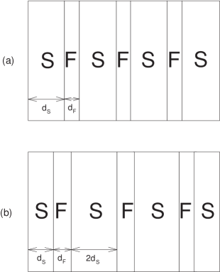
Figure 1: Examples of the two types of multilayer geometries for the heterostructures examined in this paper. The system has a total thickness $d$ in the $z$ direction, and the $F$ layers have thickness $d_{F}$. The general patterns shown hold for structures with an arbitrary odd value of the number of layers, $N_{L}$. The seven layer case is displayed. In pattern (a) the thicknesses of each S layer is $d_{S}$, while in (b) the two outer $S$ layers have thickness $d_{S}$, and the inner ones have thickness $2d_{S}$ (see text).

We consider three-dimensional slab-like heterostructures translationally invariant in the $x-y$ plane, with all spatial variations occurring in the $z$ direction. The heterostructure consists of superconducting, $S$, and ferromagnetic, $F$, layers. Examples are depicted in Fig. 1. The corresponding coupled equations for the spin-up and spin-down quasiparticle amplitudes ($u_{n}^{\downarrow},v_{n}^{\uparrow}$) then read

$$[-\frac{1}{2m}\frac{\partial^{2}}{\partial z^{2}}+\varepsilon_{\perp}-E_{F}(z)+U(z)-h_{0}(z)]u_{n}^{\uparrow}(z)+\Delta(z)v_{n}^{\downarrow}(z) =\epsilon_{n}u_{n}^{\uparrow}(z)$$ (1a)

$$-[-\frac{1}{2m}\frac{\partial^{2}}{\partial z^{2}}+\varepsilon_{\perp}-E_{F}(z)+U(z)+h_{0}(z)]v_{n}^{\downarrow}(z)+\Delta(z)u_{n}^{\uparrow}(z) =\epsilon_{n}v_{n}^{\downarrow}(z),$$ (1b)

where $\varepsilon_{\perp}$ is the kinetic energy term corresponding to quasiparticles with momenta transverse to the $z$ direction, $\epsilon_{n}$ are the energy eigenvalues, $\Delta(z)$ is the pair potential, and $U(z)$ is the potential that accounts for scattering at each $F/S$ interface. An additional set of equations for $u_{n}^{\downarrow}$ and $v_{n}^{\uparrow}$ can be readily written down from symmetry arguments, and thus is suppressed here for brevity. The form of the ferromagnetic exchange energy $h_{0}(z)$ is given by the Stoner model, and therefore takes the constant value $h_{0}$ in the $F$ layers, and zero elsewhere. Other relevant material parameters are taken into account through the variable bandwidth $E_{F}(z)$. This is taken to be $E_{F}(z)=E_{FS}$ in the $S$ layers, while in the $F$ layers one has $E_{F}(z)=E_{FM}$ so that in these regions the up and down bandwidths are respectively $E_{F\uparrow}=E_{FM}+h_{0}$, and $E_{F\downarrow}=E_{FM}-h_{0}$. The dimensionless parameter $I$, defined as $I\equiv h_{0}/E_{FM}$, conveniently characterizes the magnets’ strength, with $I=1$ corresponding to the half metallic limit. The ratio $\Lambda\equiv E_{FM}/E_{FS}\equiv(k_{FM}/k_{FS})^{2}$ describes the mismatch between Fermi wavevectors on the $F$ and $S$ sides, assuming parabolic bands with $k_{FS}$ denoting the Fermi wave vector in the $S$ regions.

The spin-splitting effects of the exchange field coupled with the pairing interaction in the $S$ regions, results in a nontrivial spatial dependence of the pair potential, which is further compounded by the normal and Andreev scattering events that occur at the multiple $S/F$ interfaces. When these complexities are taken into account, one generally cannot assume any explicit form for $\Delta(z)$ a priori. Thus, when solving Eqs. (1), the pair potential must be calculated in a self consistent manner by an appropriate sum over states:

$$\Delta(z)=\frac{\pi g(z)N(0)}{k_{FS}d}\sum_{\epsilon_{n}\leq\omega_{D}}\int{d\varepsilon_{\perp}}\left[u_{n}^{\uparrow}(z)v^{\downarrow}_{n}(z)+u_{n}^{\downarrow}(z)v^{\uparrow}_{n}(z)\right]\tanh(\epsilon_{n}/2T),$$ (2)

where $N(0)$ is the DOS per spin of the superconductor in the normal state, $d$ is the total system size in the $z$ direction, $T$ is the temperature, $\omega_{D}$ is the cutoff “Debye” energy of the pairing interaction, and $g(z)$ is the effective coupling, which we take to be a constant $g$ within the superconductor regions and zero elsewhere.

The presence of interfacial scattering is expected to modify the proximity effect. We assume that every $S/F$ interface induces the same scattering potential, which we take of a delta function form:

$$U(z_{l},z)=H\delta(z-z_{l})$$ (3)

where $z_{l}$ is the location of the interface and $H$ is the scattering parameter. It is convenient to use the dimensionless parameter $H_{B}\equiv mH/k_{FS}$ to characterize the interfacial scattering strength.

An appropriate choice of basis allows Eqs. (1) to be transformed into a finite $2N\times 2N$ dimensional matrix eigenvalue problem in wave vector space:

$$\begin{bmatrix}H^{+}&D\\ D&H^{-}\end{bmatrix}\Psi_{n}=\epsilon_{n}\,\Psi_{n},$$ (4)

where $\Psi_{n}^{T}=(u^{\uparrow}_{n1},\ldots,u^{\uparrow}_{nN},v^{\downarrow}_{n1},\ldots,v^{\downarrow}_{nN})$, are the expansion coefficients associated with the set of orthonormal basis vectors, $u^{\uparrow}_{n}(z)=\sqrt{{2}/{d}}\sum_{q=1}^{N}u^{\uparrow}_{nq}\sin(k_{q}z)$, and $v^{\downarrow}_{n}(z)=\sqrt{{2}/{d}}\sum_{q=1}^{N}v^{\downarrow}_{nq}\sin(k_{q}z)$. The longitudinal momentum index $k_{q}$ is quantized via $k_{q}={q/\pi}{d}$, where $q$ is a positive integer. The label $n$ encompasses the index $q$ and the value of $\varepsilon_{\perp}$. The finite range of the pairing interaction $\omega_{D}$, implies that $N$ is finite. In our layered geometry submatrices corresponding to different values of $\varepsilon_{\perp}$ are decoupled from each other, so one considers matrices labeled by the $q$ index, for each relevant value of $\varepsilon_{\perp}$. The matrix elements in Eq. (4) depend in general on the geometry under consideration, and are given for two specific cases in the subsections below.

II.2 Identical superconducting layers

The first type of structure we consider is one consisting of alternating $S$ and $F$ layers, each of width $d_{S}$ and $d_{F}$ respectively. This geometry is shown in Fig. 1(a) for the particular case of $N_{L}=7$. For a given total number of layers (superconducting plus magnetic) $N_{L}$, we have in this case for the interfacial scattering:

$$U(z)=\sum_{i=1}^{{(N_{L}-1)}/{2}}[U(i(d_{S}+d_{F}),z)+U((i(d_{S}+d_{F})-d_{F})),z]$$ (5)

where $U(z_{l},z)$ is given in Eq. (3). The matrix elements $H^{+}_{qq^{\prime}}$ and $H^{-}_{qq^{\prime}}$ in Eq. (4) are compactly written for this geometry as

$$H^{+}_{qq} =\frac{k^{2}_{q}}{2m}+\varepsilon_{\perp}+\frac{2H}{d}\left[\frac{N_{L}-1}{2}-A(2q)\right]-E_{F\uparrow}\left[\frac{d_{F}}{d}\left(\frac{N_{L}-1}{2}\right)+B(2q)\right]$$

$$-E_{FS}\left[\frac{d_{S}}{d}\left(\frac{N_{L}+1}{2}\right)-B(2q)\right],$$ (6a)

$$H^{+}_{qq^{\prime}} =\frac{2H}{d}[A(q-q^{\prime})-A(q+q^{\prime})]+[E_{F\uparrow}-E_{FS}][B(q-q^{\prime})-B(q+q^{\prime})], q\neq q^{\prime},$$ (6b)

where,

$$A(q) =\cos\left(\frac{d_{F}\pi q}{2d}\right)\sum_{i=1}^{(N_{L}-1)/2}\cos\left[\frac{\pi q}{2d}(2d_{S}i+d_{F}(2i-1))\right],$$ (7a)

$$B(q) =\frac{2\sin\left(\frac{d_{S}\pi q}{2d}\right)}{\pi q}\sum_{i=1}^{(N_{L}+1)/2}\cos\left[\frac{\pi q}{2d}(d_{S}(2i-1)+2d_{F}(i-1))\right].$$ (7b)

The matrix elements $H^{-}_{qq^{\prime}}$ are similarly expressed in term of the coefficients $A(q)$ and $B(q)$,

$$H^{-}_{qq} =-\frac{k^{2}_{q}}{2m}-\varepsilon_{\perp}-\frac{2H}{d}\left[\frac{N_{L}-1}{2}-A(2q)\right]+E_{F\downarrow}\left[\frac{d_{F}}{d}\left(\frac{N_{L}-1}{2}\right)+B(2q)\right]$$

$$+E_{FS}\left[\frac{d_{S}}{d}\left(\frac{N_{L}+1}{2}\right)-B(2q)\right],$$ (8a)

$$H^{-}_{qq^{\prime}} =-\frac{2H}{d}[A(q-q^{\prime})-A(q+q^{\prime})]-[E_{F\downarrow}-E_{FS}][B(q-q^{\prime})-B(q+q^{\prime})], q\neq q^{\prime}.$$ (8b)

The $D_{qq^{\prime}}$ in the off-diagonal part of the left side of Eq. (4) arise from an integral over $\Delta(z)$, which scatters a quasiparticle of a given spin into a quasihole of opposite spin. One has:

$$D_{qq^{\prime}}=\frac{2}{d}\int_{0}^{d}dz\sin(k_{q}z)\Delta(z)\sin(k_{q}^{\prime}z).$$ (9)

It is straightforward to write alsohv2 ; hv3 the self consistency equation in terms of matrix elements.

II.3 Half-width superconducting outer layers

The previous subsection outlined the details needed to arrive at the matrix elements when the $S$ layers are of the same width $d_{S}$. We are also interested in investigating structures where the inner $S$ layers are twice as thick ($2d_{S}$) as the outer ones (see Fig. 1(b)) while the $F$ layers remain all of the same width. This case is of interest because, roughly speaking, the inner layers, being between ferromagnets, should experience about twice the pair-breaking effects of the exchange field than do the outer ones. Therefore, the results might depend on $N_{L}$ more systematically, particularly for relatively small $N_{L}$, if the witdth of the outer layers is halved. This has been found to be the case in some studiesprosh of the transition temperature in thin layered systems.

A slight modification to the previous results yields the following form of the scattering potential $U(z)$,

$$U(z)=\sum_{i=1}^{{(N_{L}-1)}/{2}}[U((i(2d_{S}+d_{F})-d_{S}),z)+U((i(2d_{S}+d_{F})-d_{S}-d_{F}),z)]$$ (10)

The matrix elements $H^{+}_{qq^{\prime}}$ are now expressed as

$$H^{+}_{qq^{\prime}} =\frac{2H}{d}[A(q-q^{\prime})-A(q+q^{\prime})]+[E_{F\uparrow}-E_{FS}][B(q+q^{\prime})-B(q-q^{\prime})],\qquad q\neq q^{\prime}$$ (11a)

$$H^{+}_{qq} =\frac{k^{2}_{q}}{2m}+\varepsilon_{\perp}+\frac{2H}{d}\left[\frac{N_{L}-1}{2}-A(2q)\right]-E_{F\uparrow}\left[\frac{d_{F}}{d}\left(\frac{N_{L}-1}{2}\right)-B(2q)\right]$$

$$-E_{FS}\left[\frac{d_{S}}{d}\left(N_{L}-1\right)+B(2q)\right],$$ (11b)

where the coefficients $A(q)$ and $B(q)$ now read,

$$A(q)=\cos\left(\frac{d_{F}\pi q}{2d}\right)\sum_{i=1}^{(N_{L}-1)/2}\cos\left[\frac{\pi q}{2d}(2i-1)(2d_{S}+d_{F})\right],\qquad B(q)=\frac{2A(q)}{\pi q}\tan\left(\frac{d_{F}\pi q}{2d}\right).$$ (12)

In a similar manner, The matrix elements $H^{-}_{qq^{\prime}}$ are written as

$$H^{-}_{qq} =-\frac{k^{2}_{q}}{2m}-\varepsilon_{\perp}-\frac{2H}{d}\left[\frac{N_{L}-1}{2}-A(2q)\right]+E_{F\downarrow}\left[\frac{d_{F}}{d}\left(\frac{N_{L}-1}{2}\right)-B(2q)\right]$$

$$+E_{FS}\left[\frac{d_{S}}{d}\left(N_{L}-1\right)+B(2q)\right],$$ (13a)

$$H^{-}_{qq^{\prime}} =-\frac{2H}{d}[A(q-q^{\prime})-A(q+q^{\prime})]-[E_{F\downarrow}-E_{FS}][B(q+q^{\prime})-B(q-q^{\prime})],\qquad q\neq q^{\prime}$$

The matrix elements of $D$ are as in the previous subsection, and the self consistent equation can be similarly rewritten.

II.4 Spectroscopy

Experimentally accessible information regarding the quasiparticle spectra is contained in the local density of one particle excitations in the system. The local density of states (LDOS) for each spin orientation is given by

$${N}_{\sigma}(z,\epsilon)=-\sum_{n}\Bigl{\{}[u^{\sigma}_{n}(z)]^{2}f^{\prime}(\epsilon-\epsilon_{n})+[v^{\sigma}_{n}(z)]^{2}f^{\prime}(\epsilon+\epsilon_{n})\Bigr{\}}.$$ (14)

where $\sigma=\uparrow,\downarrow$ and $f^{\prime}(\epsilon)=\partial f/\partial\epsilon$ is the derivative of the Fermi function.

As discussed in the Introduction, the condensation free energies of the different self consistent solutions found must be comparedhv3 in order to find the most stable configuration, as opposed to those that are metastable. While for homogeneous systems this quantity is found in standard textbooks,tinkham ; fw . the case of an inhomogeneous system is more complicated. We will use the convenient expression found in Ref. kos, for the free energy ${\cal F}$:

$${\cal F}=-2T\sum_{n}{\ln\left[2\cosh\left(\frac{\epsilon_{n}}{2T}\right)\right]}+\int^{d}_{0}dz\frac{|\Delta(z)|^{2}}{g},$$ (15)

where the sum can be taken over states of energy less than $\omega_{D}$. For a uniform system the above expression properly reduces to the standard textbook result.fw The corresponding condensation free energy (or, at $T=0$, the condensation energy) is obtained by subtracting the corresponding normal state quantity, as discussed below. Thus, in principle, only the results for $\Delta(z)$ and the excitation spectra are needed to calculate the free energy. As pointed out in Ref. hv3, , a numerical computation of the condensation energies that is accurate enough to allow comparison between states of different types requires great care and accuracy. Details will be given in the next section.

III Results

As explained in the Introduction, the chief objective of this work is to study the relative stability of the different states that are obtained through self-consistent solution of the BdG equations for this geometry. These solutions differ in the nature of the junctions. Each junction between two consecutive S layers can be of the “0” type (with the order parameter in both S layers having the same phase) or of the “$\pi$” type (opposite phase). As the number of layers, and junctions, increases, the number of order parameter (or junction) configurations which are in principle possible increases also. As we shall see, for any set of parameter values (geometrical and material) not all of the possible configurations are realized: some do not correspond to free energy local minima. Among those that do, the one (except for accidental degeneracies) which is the absolute stable minimum must be determined, the other ones being metastable. We will discuss these stability questions as a function of the material and geometrical properties, as represented by dimensionless parameters as we shall now discuss.

III.1 General considerations

Three material parameters are found to be very important: one is obviously the magnet strength $I$. We will vary this parameter in the range from zero to one, that is, from nonmagnetic to half-metallic. The second is the wavevector mismatch characterized by $\Lambda\equiv(k_{FM}/k_{FS})^{2}$. The importance of this parameter can be understood by considering that, even in the non self consistent limit, the different amplitudes for ordinary and Andreev scattering depend strongly on the wavevectors involved, as it follows from elementary considerations. We will vary $\Lambda$ in the range from unity (no mismatch) down to $1/10$. We have not considered values larger than unity as these are in practice infrequent. The third important dimensionless parameter is the barrier height $H_{B}$ defined below Eq. (3). This we will vary from zero to unity, at which value the $S$ layers become, as we shall see, close to being decoupled. We will keep the superconducting correlation length fixed at $k_{FS}\xi_{0}\equiv\Xi_{0}=100$. This quantity sets the length scale for the superconductivity and therefore can be kept fixed, recalling only that, to study the $d_{S}$ dependence, one needs to consider the value of $d_{S}/\xi_{0}$. Finally the cutoff frequency $\omega_{D}$ can be kept fixed (we set $\omega_{D}=0.04E_{FS}$) since it sets the overall energy scale and we are interested in relative shifts. The dimensionless coupling constant $gN(0)$ can be derived from these quantities using standard relations. In this study we will focus on very low temperatures limit, fixing $T$ to $T=0.01T_{C}^{0}$ (where $T_{C}^{0}$ is the bulk transition value). The geometrical parameters are obviously the number of layers $N_{L}$, and the thicknesses $d_{F}$ and $d_{S}$. We will consider two examples of the first: $N_{L}=3$ and $N_{L}=7$. For the larger value we will study both of the geometries in panels (a) and (b) of Fig. 1. The thicknesses, usually expressed in terms of the dimensionless quantities $D_{S}\equiv k_{FS}d_{S}$ and $D_{F}\equiv k_{FS}d_{F}$, will be varied over rather extended ranges.

As we study the effect of each one of these parameters by varying it in the appropriate range, we will be holding the others constant at a certain value. Unless otherwise indicated, the values of the parameters held constant will take the “default” values $I=0.2$, $D_{S}=100=\Xi_{0}$, $D_{F}=10$, $\Lambda=1$, and $H_{B}=0$. One important derived length is $(k_{\uparrow}-k_{\downarrow})^{-1}$, where $k_{\uparrow}$ and $k_{\downarrow}$ are the Fermi wavevectors of the up and down magnetic bands. As is well knowndab ; hv1 , this quantity determines the approximate spatial oscillations of the pair amplitude in the magnet. In terms of the quantities $I$ and $\Lambda$ we can define:

$$\Xi_{2}\equiv k_{FS}(k_{\uparrow}-k_{\downarrow})^{-1}=\frac{1}{\Lambda^{1/2}}\frac{1}{\sqrt{(1+I)}-\sqrt{(1-I)}}$$ (16)

At $I=0.2$ and $\Lambda=1$ one has $\Xi_{2}=4.97$ increasing to $15.7$ at $\Lambda=0.1$. This motivates our default choice $D_{F}=10$.

The numerical algorithm used in our self consistent calculations follows closely that of previous developed codes used in simpler geometries.hv2 ; hv3 There are however some extra complexities that arise for the larger multilayered structures studied here, and from the increased number of self consistent states to be analyzed. As usual, one must assume an initial particular form for the pair potential, to start the iteration process. This permits a straightforward diagonalization of the matrix given in Eq. (4) for a given set of geometrical and material parameters, for each value of the transverse energy $\varepsilon_{\perp}$. The initial guess of $\Delta(z)$ is always chosen as a piecewise constant $\pm\Delta_{0}$, where $\Delta_{0}$ is the zero temperature bulk gap, and the signs depend on the possible configuration being investigated (see below). Self consistency is deemed to have been achieved when the difference between two successive $\Delta(z)$’s is less than $10^{-5}\Delta_{0}$ at every value of $z$. The minimum number of $\varepsilon_{\perp}$ variables needed for self consistency is around $N_{\perp}=500$ different values of $\varepsilon_{\perp}$. In practice however, use of a value close to this minimum is insufficient to produce smooth results for the local DOS. Therefore, we first calculate $\Delta(z)$ self consistently using $N_{\perp}=500$, after which iteration is continued with $N_{\perp}$ increased by a factor of ten. The computed spectra then summed according to Eq. (14) are smooth and further increases in $N_{\perp}$ produce no discernible change in the outcome. This two-step procedure leads to considerable savings in computer time. The convergence properties and net computational expense obviously depend also on the dimension of the matrix to be diagonalized, dictated by the number of basis functions, $N$, which scales linearly with system size $k_{FS}d$. Thus, the computational time then increases approximately as $(k_{FS}d)^{2}$, which can be a formidable issue. For the largest structures considered in this paper, the resultant matrix dimension is then $2N\times 2N\simeq 2000\times 2000$ for each $\varepsilon_{\perp}$.

The number of iterations needed for self consistency depends on the initial guess. If the self consistent state turns out to be composed of junctions of the same types as the initial guess, as specified by the signs in the $\pm\Delta_{0}$, then forty or fifty iterations are usually sufficient. But a crucial point is that, as we shall see, not all of the initial junction configurations lead to self consistent solutions of the same type. Since the self-consistency condition is derived from a free energy minimization condition, this means that some of the initial guesses do not lead to minima in the free energy with the same junction configuration as the initial guess, and thus that locally stable states of that type do not exist, for the particular parameter values studied. In this case, the number of iterations required to get a self consistent solution increases dramatically, since the pair potential has to reconfigure itself into a much different profile. The number of iterations in those cases can exceed 400.

The computation of the condensation free energies of the self consistent states found is still a difficult task, even after the spectra are computed: considering for illustration the $T=0$ limit, recalltinkham that the bulk condensation energy, given by

$$E_{0}^{b}=-(1/2)N(0)\Delta_{0}^{2}$$ (17)

represents a fraction of the energy of the relevant electrons of order $(\Delta/\omega_{D})^{2}$, a quantity of order $10^{-2}$ or less. The condensation free energies of the inhomogeneous states under discussion are usually much smaller (by about an order of magnitude as we shall see) than that of the bulk. Distinguishing among competing states by comparing their often similar condensation free energies, requires computing these individual condensation energies to very high precision. This task is numerically difficult. Here the advantages of the expression from Ref. kos, which we use (see Eq. (15)) are obvious. Only the energies are explicitly needed in the sums and integrals on the right side, the influence of the eigenfunctions being only indirectly felt through the relatively smooth function $\Delta(z)$. The required quantities are obtained with sufficient precision, as we shall demonstrate, from our numerical calculations. Some of the different but equivalent expressions found in the literature for the condensation energies or free energiesfw ; ks , contain explicit sums over eigenfunctions, which can lead to cumulative errors. Also, the approximate formula used for the condensation energy of trilayers in Ref. hv3, , consisting in replacing, in Eq. (17), the pair amplitude with its spatial average, while plausible, is difficult to validate in general, and becomes inaccurate for systems involving a larger number of thinner layers, particularly with $S$ widths of order of $\xi_{0}$.

Using this procedure, the task then becomes feasible but not trivial as it involves a sum over more than $10^{6}$ terms. Also, to obtain the condensation energy one still has to subtract from the superconducting ${\cal F}$ the corresponding normal quantity ${\cal F_{N}}$. It is from subtracting these larger quantities that the much smaller condensation free energy is obtained. The normal state energy spectra used to evaluate ${\cal F_{N}}$ are computed by taking $D=0$ in Eq. (4), and diagonalizing the resulting matrix. The presence of interfacial scattering and mismatch in the Fermi wavevectors still introduces off-diagonal matrix elements. In performing the subtraction, care must be taken (as in fact is also the case in the bulk analytic case) to include exactly the same number of states in both calculations, rather than loosely using the same energy cutoff: no states overall are created or lost by the phase transition. With all of these precautions, results of sufficient precision and smoothness are obtained. Results obtained with alternative equivalentbkk formulas are consistent but noisier. We have verified that in the limiting case of large superconducting slabs our procedure reproduces the analytic bulk results.

III.2 Pair amplitude

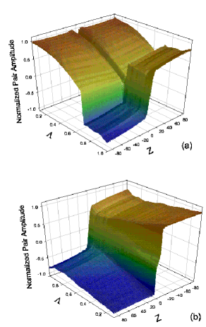
Figure 2: (Color online). The pair amplitude $F(Z)$, normalized to $\Delta_{0}$, for a three layer $SFS$ structure, plotted as a function of $Z\equiv k_{FS}z$ and of the mismatch parameter $\Lambda$, at $H_{B}=0$. The direction of the $\Lambda$ scale is different in the top and bottom panels. The $Z=0$ point is at the center of the structure. We have $D_{S}\equiv k_{FS}d_{S}=100$ and $D_{F}\equiv k_{FS}d_{F}=10$. Panel (a) corresponds to self consistent results obtained with an initial guess where the junction is of the “0” type and panel (b) with a “$\pi$” type. In the latter case, the solution found is always of the $\pi$ type, but in the former a solution of the 0 type is obtained only for large mismatch (small $\Lambda$). We have $I=0.2$ and $T=0.01T_{c}^{0}$ here. See text for discussion.

We begin by presenting some results for the pair amplitude $F(z)$, showing how this quantity varies as a function of the interface scattering parameter $H_{B}$ and the Fermi wavevector mismatch $\Lambda$. This is best done by means of three dimensional plots. In the first of these, Fig. 2, we show the pair amplitude (normalized to $\Delta_{0}$) for a three layer $SFS$ system, with $D_{F}=10$ and $D_{S}=100$, as a function of position and of mismatch parameter $\Lambda$, at $H_{B}=0$. The top panel shows the results of attempting to find a solution of the “0” type by starting the iteration process with an initial guess of that form. Clearly such an attempt fails at small mismatch ($\Lambda\gtrsim 0.7$) indicating that a solution of this type is then unstable. At larger mismatch, a $0$ state solution is found. Panel (b) shows solutions obtained by starting with an initial guess of the “$\pi$” type: a self consistent solution of this type is then always obtained (note that the $\Lambda$ scales run in different directions in panels (a) and (b)). For $\Lambda\gtrsim 0.7$, the solutions of course turn out to be the same as found in panel (a) in the same range. Thus, we see that for small mismatch there is only one self consistent solution, which is of the $\pi$ type, while when the mismatch is large there are two competing solutions and their relative stability becomes an issue.

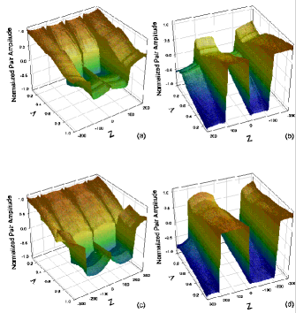
Figure 3: (Color online). The normalized pair amplitude $F(Z)$ for a seven layer $SFSFSFS$ structure, plotted as in Fig. 2 for the same parameter values. In panels (a) and (b), the thickness of all S layers is the same, while in panels (c) and (d) the thickness of the two inner S layers is doubled to $2D_{S}=200$ (see Fig. 1). Panels (a) and (c) correspond to an initial guess of the “000” type and panels (b) and (d) to a “$\pi\pi\pi$” type, (see text). The configuration of the plotted self consistent results can be “000”, “$\pi\pi\pi$” or “$\pi 0\pi$” as explained in the text.

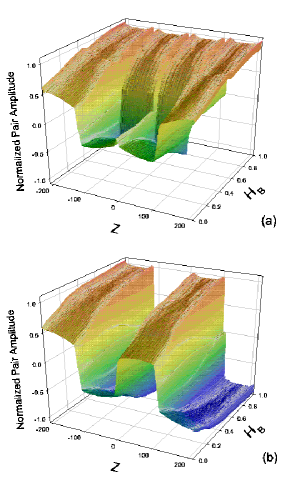
Figure 4: (Color online). The pair amplitude $F(Z)$ for a seven layer structure, plotted for the same parameter values and conventions as in the upper panels of Fig. 2, but as a function of the dimensionless barrier height $H_{B}$ (at $\Lambda=1$), rather than of the mismatch.

We now turn to seven layer $SFSFSFS$ structures. In classifying the different possible configurations, it is convenient to establish a notation that envisions the seven layer geometry as consisting of three adjacent $SFS$ junctions. Thus, up to a trivial reversal, we can then denote as “$000$” the structure when adjacent $S$ layers always have the same sign of $\Delta(z)$, and as “$\pi\pi\pi$” the structure where successive $S$ layers alternate in sign. There are also two other distinct symmetric states: one in which $\Delta(z)$ has the same sign in the first two $S$ layers, and in the last two it has the opposite sign, (this is labeled as the “$0\pi 0$” configuration), and the other corresponding to the two outer $S$ layers having the same sign for $\Delta(z)$, opposite to that of the two inner $S$ layers: these are referred to as “$\pi 0\pi$” structures in this notation. We will focus our study on these symmetric configurations. Asymmetric configurations corresponding in our notation to the $\pi 00$, and $\pi\pi 0$ states are not forbidden, but occur very rarely and will be addressed only as need may arise. In Fig. 3 we repeat the plots in Fig. 2 for seven layer structures. We include the cases in which all $S$ layers are of the same thickness (top two panels) and the case where the thickness of the two inner $S$ layers is doubled (bottom panels, see Fig. 1). In panels (a) and (c), the initial guess is of the $000$ type, while in (b) and (d) it is of the $\pi\pi\pi$ type. In the case of identical $S$ layer widths, we see that a $000$ guess (Fig. 3(a)) yields a self consistent state of the same $000$ form only for larger mismatch, $\Lambda\lesssim 0.5$, while for smaller mismatch the configuration obtained is clearly of the $\pi 0\pi$ form. Thus there is a value of $\Lambda$ where two self consistent solutions cross over. However, a $\pi\pi\pi$ guess (Fig. 3(b)) results in a self consistent $\pi\pi\pi$ configuration for the whole $\Lambda$ range. Thus, there is a clear competition between at least these three observed states, resulting from multiple minima of the free energy. Solutions of the $0\pi 0$ type are not displayed in this Figure but they will be discussed below. In the two bottom panels we see the same effects when the thickness of the inner S layers is doubled. As explained above, this describes a more balanced situation, since the inner layers have magnetic neighbors on both sides. It is evident from the figure that the pairing correlations are increased in the $S$ layers. In Fig. 3(c), there is also a noticeable shift in the crossover point separating the $000$ and $\pi 0\pi$ self consistent states, occurring now at smaller mismatch $\Lambda\approx 0.7$. Again we find the competition between the various states extends through the entire range of $\Lambda$ considered.

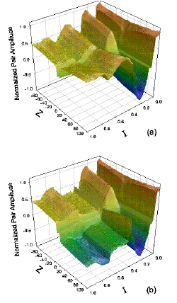
Figure 5: (Color online). The pair amplitude $F(Z)$ for a three layer structure, plotted for the same parameter values and conventions as in Fig. 2, but as a function of the dimensionless magnetic polarization $I$, at $\Lambda=1$ and $H_{B}=0$.

Next we consider in Fig. 4 the influence of the barrier height as represented by the dimensionless parameter $H_{B}$. This figure is completely analogous to Fig. 3(a) and (b), except for the substitution of $H_{B}$ for $\Lambda$, which is set to unity (no mismatch). We find, by examining and comparing the panels that two solutions of the $\pi\pi\pi$ and $\pi 0\pi$ type exist for small barrier heights ($H_{B}\lesssim 0.5$), but when $H_{B}$ becomes larger the $\pi\pi\pi$ and $000$ states then compete. Another trend which one can clearly discern is that the absolute values of $F(Z)$ in the middle of the S layers increase with $H_{B}$. This makes sense, as at larger barrier heights the layers become more isolated from each other, and the proximity effects must in general weaken.

To conclude this discussion of $F(z)$ we display in Fig. 5, the pair amplitude for the same three layer system as in Fig. 2, as a function of position and of the magnetic exchange parameter $I$ in its entire range, without a barrier or mismatch. Careful examination of the two panels reveals a rather intricate situation: a solution of the $\pi$ type exists nearly in the entire $I$ range (see Fig. 5(b)), the exception being at very small $I$, where the magnetism becomes weaker and, as one would expect, only the $0$ state solution is found. This requires small values of $I$, $I\lesssim 0.1$ however. One can see that in a small neighborhood of $I\approx 0.1$, as the $0$ state transitions to the $\pi$ state, the pair amplitude is small throughout the structure. This may correspond to a marked dip in the transition temperature. At larger values of $I$, the two types of solutions coexist, but there is a range around $I=0.2$ where clearly there is only one.

These results, which include for brevity only a very small subset of those obtained, are sufficient, we believe, to persuade the reader that although for some parameter values a unique self consistent solution exists, this is comparatively rare, and that in general several solutions of differing symmetry types can be found. These self consistent solutions correspond to local free energy minima: they are at least metastable. Furthermore, it is clear that the uniqueness or multiplicity of solutions depends in a complicated way not only on the geometry, but also on the specific material parameter values.

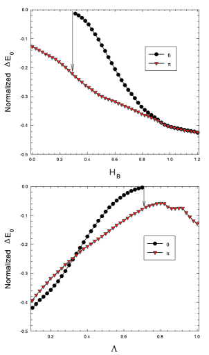
Figure 6: (Color online). The normalized condensation free energy $\Delta E_{0}$ (see text) of a three layer $SFS$ structure, plotted as a function of barrier height (top) and mismatch parameter $\Lambda$ (bottom) for self consistent states of both the 0 and $\pi$ types, as indicated. All other material parameters, geometrical values, and temperature, are as in Fig. 2. The vertical arrow marks the end, as either $H_{B}$ increases (top) or $\Lambda$ increases (bottom), of the region of stability of the 0 state in this case.

III.3 Condensation Free Energy: Stability

One must, in view of the results in the previous subsection, find a way to determine in each case the relative stability of each configuration and the global free energy minimum. This is achieved by computing the free energy of the several self consistent states, using the accurate numerical procedures explained earlier in this Section. Results for this quantity, which at the low temperature studied is essentially the same as the condensation energy, are given in the next figures below. The quantity plotted in these figures, which we call the normalized $\Delta E_{0}$, is the condensation free energy (as calculated from Eq. (15) after normal state subtraction) normalized to $N(0)\Delta_{0}^{2}$, which is twice the zero temperature bulk value (see Eq. 17). Therefore, at the low temperatures studied, the bulk uniform value of the quantity plotted is very close to $-(1/2)$.

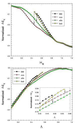
Figure 7: (Color online). The normalized $\Delta E_{0}$ for a seven layer $SFSFSFS$ structure plotted as a function of barrier height (top) and mismatch parameter $\Lambda$ (bottom) for self consistent states of the types indicated (see text for explanation). Material parameter and geometrical values are as in previous Figures, and all $S$ layers are of the same thickness. The vertical arrows mark the end, as $H_{B}$ decreases (top) or $\Lambda$ increases (bottom, see inset) of the region of stability of a certain state (see text).

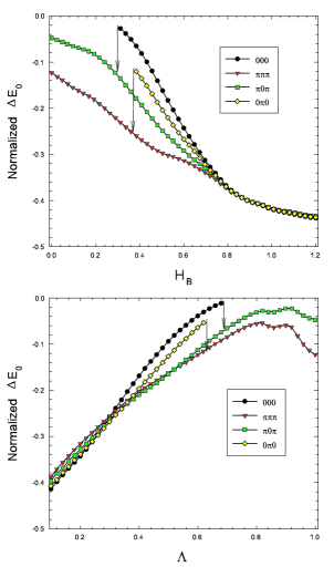
Figure 8: (Color online). Normalized $\Delta E_{0}$ for a seven layer $SFSFSFS$ structure, as in Fig. 7, but for the case where the thickness of the two inner S layers is doubled.

In Figure 6 we plot $\Delta E_{0}$, defined and normalized as explained, for a three layer $SFS$ system. As in previous Figures, we have $D_{S}=100$, $D_{F}=10$ and $I=0.2$. Results for self consistent states of both the 0 and $\pi$ type are plotted as indicated. The top panel shows $\Delta E_{0}$ as a function of the barrier thickness parameter $H_{B}$ at $\Lambda=1$. The bottom panel plots the same quantity as a function of mismatch $\Lambda$ at zero barrier and should be viewed in conjunction with Fig. 2. Looking first at the top panel, one sees that the zero state is stable (has nonzero condensation energy) only for $H_{B}$ greater than about $0.31$. An attempt to find a solution of the 0 type for $H_{B}$ just below its “critical” value by using a solution of that type previously found for a slightly higher $H_{B}$ as the starting guess, and iterating the self consistent process, leads after many iterations to a solution of the $\pi$ type. This is indicated by the vertical arrow. At larger barrier heights, the two states become degenerate. This makes sense physically: as the barriers become higher the proximity effect becomes less important, and the S layers behave more as independent superconducting slabs. The relative phase is then immaterial. For even larger $H_{B}$ we expect, from Eq. 17 and the geometry, the normalized quantity plotted to trend, from above, toward a limit $\approx-0.5(1-D_{F}/D_{S})=-0.45$ and this is seen in the top panel. One can also see that in the region of interest (barriers not too high), the absolute value of the condensation energy is substantially below that of the bulk. In the bottom panel similar trends can be seen: in the absence of mismatch ($\Lambda=1$) only the $\pi$ state is found, and its condensation energy exhibits a somewhat oscillatory behavior as $\Lambda$ decreases from unity. The 0 state does not appear until $\Lambda$ is about $0.7$ and attempts (by the procedure just described) to find it lead to a $\pi$ solution upon iteration (arrow). This is in agreement with the results in Fig. 2. For large mismatch the absolute value of $\Delta E_{0}$ increases, as the S slabs become more weakly coupled, with a trend toward the limiting value just discussed. A very important difference between the top and bottom panels, however, is the crossing of the curves near $\Lambda=0.33$ in Fig. 6(b). This is in effect a first order phase transition between the $\pi$ and 0 configurations as the mismatch changes.

The results of performing the same study for a seven layer system with four $S$ layers can be seen in the next two Figures. Figure 7 corresponds to the case where all the $S$ layers have the same thickness ($D_{S}=100$, and all other parameters also as in the previous figures), while in Fig. 8 the thickness of the two inner $S$ layers is doubled. Results for the four possible symmetric junction configurations mentioned in conjunction with Fig. 3 are given, as indicated in the legends of Figs. 7 and 8. Three of those configurations, $000$, $\pi\pi\pi$ and $\pi 0\pi$ have appeared among the results in Figs. 3 and 4. The other configuration corresponds to the $0\pi 0$ sequence.

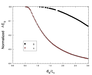
Figure 9: (Color online). The normalized $\Delta E_{0}$ for a three layer $SFS$ system, as a function of the thickness $d_{S}$ of the $S$ layers (given in units of $\xi_{0}$) at fixed $D_{F}=10$, $I=0.2$ and without a barrier or mismatch. Results for 0 and $\pi$ self consistent states are given as indicated.

We see that there are some striking differences between these examples and the three layer system. While in the latter case a configuration ceases to exist only when its condensation energy tends to zero, now configurations can become unstable even when, for nearby values of the relevant parameter, they still have a negative condensation energy. As this occurs, the vertical arrows in each panel indicate (an inset is needed in one case for clarity) how the states transform into each other as one varies the parameters from the unstable to the stable region. Regardless of whether the inner layers are doubled or not, the tendency is for the innermost junction to remain of the same type, while the two outer junctions flip. Comparing Fig. 7 and Fig. 8 we see that the doubling of the inner layers has a clear quantitative effect without having any strong qualitative influence. An important difference between the two cases is that in the first (all $S$ layer widths equal) the two possible states ($\pi 0\pi$ and $\pi\pi\pi$) at zero barrier and no mismatch are nearly degenerate, while in the other case, the $\pi\pi\pi$ configuration is favored. In the first case, the degeneracy is removed as the barrier height begins to increase, but $\Lambda$ has a small effect in relative stability. In Fig. 8, bottom panel, the oscillatory effect of $\Lambda$ near the no-mismatch limit is seen, as in the three layer case. For large mismatch or barrier, the results become again degenerate and trend towards the appropriate limit. We expect these seven layer results to be at least qualitatively representative of what occurs for larger values of $N_{L}$: thus, states of the types $000\cdots 000$, $\pi\pi\cdots\pi\pi$, and $\pi 00\cdots 00\pi$ (outer junctions one way and inner ones the other) should predominate for large $N_{L}$.

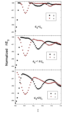
Figure 10: (Color online). The normalized $\Delta E_{0}$ for a three layer $SFS$ junction, as a function of the parameter $I$, for three different $S$ thicknesses (as labeled) and fixed $D_{F}=10$. Results for 0 and $\pi$ self consistent states are given as indicated.

It is at least of equal interest to study how the stability depends on the geometry. We discuss this question in the next four figures. First, in Fig. 9 we present results for the condensation free energy of a three layer system as a function of $d_{S}/\xi_{0}$ at fixed $D_{F}=10$, $I=0.2$, $H_{B}=0$, $\Lambda=1$. We see that $d_{S}$ must be at least half a correlation length for superconductivity to be possible at all in this system. Convergence near that value is rather slow, requiring approximately 200 iterations. The superconducting state then begins occurring, for this value of $D_{F}$, in a $\pi$ configuration only. When $d_{S}$ reaches $\xi_{0}$, the $\pi$ state condensation energy reaches already an appreciable value that is consistent with that seen in the appropriate limits of the panels in Fig. 6. The $0$ state is still not attainable (again, consistent with Fig. 6) until $d_{S}$ reaches a somewhat larger value. The condensation energies of the two states converge slowly toward each other upon increasing $d_{S}$, but remain clearly non-degenerate well beyond the range plotted. The small breaks in the $0$ state curve correspond to specific $S$ widths that permit only the $\pi$ state.

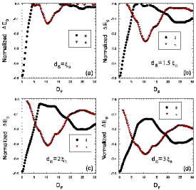
Figure 11: (Color online). The normalized $\Delta E_{0}$ for a three layer $SFS$ system, as a function of $d_{F}$, (rather than of $I$ as in Fig. 10) for four different $S$ thicknesses (as labeled) and fixed $I=0.2$, $H_{B}=0$, $\Lambda=1$.

The behavior seen in Fig. 9 depends strongly on $I$. This dependence is displayed in Fig. 10 where we show the normalized $\Delta E_{0}$ for the same system, as a function of $I$, for three different values of $d_{S}$. For the value $I=0.2$, the results shown are consistent with Fig. 9, including the nonexistence of the 0 state at $d_{S}=\xi_{0}$. We now see, however, that it is not always the $\pi$ state which is favored, but that the difference in condensation energies is an oscillatory function of $I$. This of course reflects that whether the 0 or the $\pi$ state is preferred depends, all other things being equal, on the relation between $D_{F}$ and $(k_{\uparrow}-k_{\downarrow})^{-1}$, and this quantity (see Eq. (16)) depends on $I$. At intermediate values of $I$ (centered around $I=0.5$) the zero state is favored, and when $I$ becomes very small the $\pi$ state ceases to exist altogether (this can be seen also by examination of Fig. 5). As $I\rightarrow 0$ the condensation energy of the 0 state remains somewhat above the bulk value and, as one would expect, decreases slightly with increasing $d_{S}$. At larger values of $I$, the absolute values of $\Delta E_{0}$ increase with $d_{S}$ and on the average decrease slowly with $I$.

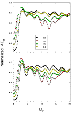
Figure 12: (Color online). The normalized condensation free energy for a seven layer $SFSFSFS$ system, as a function of $D_{F}$, for fixed $I=0.2$, $d_{S}=\xi_{0}$, $\Lambda=1$ and $H_{B}=0.5$. Results for the four possible symmetric self consistent states are given, as indicated, for both the cases where all $S$ layers are identical (top) and where the thickness of the inner ones is doubled (bottom). Lines are guides to the eye. Breaks (top panel) indicate regions where a certain configuration is not found.

The oscillations in Fig. 10 as a function of $I$ at constant $d_{F}$ can also be displayed by considering results as a function of $d_{F}$ at constant $I$. We do so in Fig. 11 where we plot, for a three layer $SFS$ system, $\Delta E_{0}$ as a function of $D_{F}$ at constant $I=0.2$ for four values of $d_{S}/\xi_{0}$. One sees again that for this value of $I$ the 0 state does not exist at $d_{S}=\xi_{0}$ and $D_{F}=10$ but that it appears at larger values of $d_{S}/\xi_{0}$. The damped oscillatory behavior is quite evident. At larger values of $d_{F}$ the condensation energies of the two states trend towards a common value that increases in absolute value with $d_{S}$. At a very small value of $d_{F}$, which depends on $d_{S}$, the $\pi$ state begins to vanish, and the condensation free energy of the 0 state tends then towards the bulk value. All of this is consistent with simple physical arguments.

In Fig. 12 we extend the results of Fig. 11 to the seven layer system. In this case we consider only one value of $d_{S}$ ($d_{S}=\xi_{0}$) but include a finite barrier thickness, $H_{B}=0.5$. The finite barrier allows for the possibility of more distinct states coexisting (see Figs. 7-8). We consider both the cases where all $S$ layers thicknesses are equal (top panel) and the case where the inner ones are doubled (bottom panel). All possible symmetric self consistent states were studied, as indicated in the figure. In contrast with the three layer example with no barrier, in the seven layer cases with $H_{B}=0.5$ all of the four symmetric states ($000,\pi\pi\pi,\pi 0\pi,0\pi 0$) are at least metastable over a range of $d_{F}$, even at $d_{S}=\xi_{0}$. In the top panel we see however that only the $0\pi 0$ state is stable over the whole $d_{F}$ range. The $\pi\pi\pi$ state reverts to the $0\pi 0$ state in the range $1.6\lesssim d_{F}\lesssim 4.2$, while the $\pi 0\pi$ state reverts to $000$ state for $1.8\lesssim d_{F}\lesssim 2.4$. The $000$ state is unstable for much of the range for $6\lesssim d_{F}\lesssim 12$. It appears that in this range the $000$ state is sufficiently close to a crossover (see e.g. Fig. 7) that attempts to find it sometimes converge to an asymmetric $\pi 00$ state, rather than the expected $\pi 0\pi$. In these cases the number of iterations to convergence is substantially increased, as the order parameter attempts to readjust its profile. For the situation where the inner $S$ layers are twice the width of the outer ones, we see (bottom panel) that all four symmetric configurations are either stable or metastable for the whole $d_{F}$ range. This is consistent with Fig. 7, where at $H_{B}=0.5$ all four states are present simultaneously. The condensation energy is of course lower than in the previous case, due to the increased pairing correlations associated with the thicker $S$ slabs. For both geometries oscillations arising from the scattering potential lead to deviations from the estimated periodicity determined by $(k_{\uparrow}-k_{\downarrow})^{-1}$. For sufficiently large $d_{F}$ the difference in energies becomes small. One can infer from these results than in superlattices with realistic oxide barriers, where as the number of layers increases a larger number of nontrivial possible states arise, the number of local free energy minima that can coexist will increase.

III.4 DOS

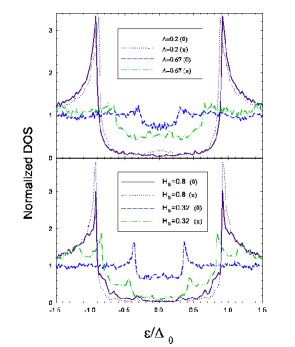
Figure 13: (Color online). The normalized DOS (see text) for a $SFS$ trilayer, plotted as a function of the energy (in units of the bulk zero temperature gap). Results for both 0 and $\pi$ self consistent states are given, as indicated. In the top panel, the DOS is shown at $H_{B}=0$ for two different values of the mismatch parameter, $\Lambda=0.2$, and 0.67, the latter being a case for which the 0 state is nearly unstable (see Fig. 6). The bottom panel shows the DOS profile in the absence of mismatch ($\Lambda=1$), but with the interface scattering parameter $H_{B}$ taking on the two values shown, chosen on similar criteria as the $\Lambda$ values (see text).

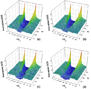
Figure 14: (Color online). The normalized local DOS for a seven layer system versus the dimensionless energy and mismatch parameter $\Lambda$. The panels are arranged as those in Fig. 3: (a) and (b) show results obtained when all $S$ layers have the same thickness, while in (c) and (d) that thickness is doubled. Panels (a) and (c) correspond to starting the iteration procedure with a $000$ order parameter, while panels (b) and (d) are obtained by starting with a $\pi\pi\pi$ junction, in which case the self-consistent solution is also always of this type.

We conclude this section by presenting some results for the DOS, as it can be experimentally measured. The results given are in all cases for the quantity ${N}_{\sigma}(z,\epsilon)$ defined in Eq. (14), summed over $\sigma$, and integrated over a distance of one coherence length from the edge of the sample. We normalize our results to the corresponding value for the normal state of the superconducting material, and the energies to the bulk value of the gap, $\Delta_{0}$. All parameters not otherwise mentioned are set to their “default” values outlined at the beginning of this section.

In the top panel of Fig. 13 we present results for an $SFS$ trilayer, for two contrasting values of the mismatch parameter $\Lambda$. As usual, results labeled as “0” and “$\pi$” are for the case where the self consistent states plotted are of these types. The $0$ and $\pi$ state curves corresponding to $\Lambda=0.67$, where (see Fig. 6) the 0 state is barely metastable, have clearly distinct signatures, with a smaller gap opening for the $0$ state, and consequently more subgap quasiparticle states. Therefore, as can be seen in Fig. 2, when there is little mismatch the pair amplitude is relatively large in the $F$ layer. When there is more mismatch the proximity effect weakens, the gap opens and large peaks form which progressively become more BCS-like as the mismatch increases ($\Lambda$ decreases) to $\Lambda=0.2$. This progression takes a different form for the 0 and $\pi$ states, as one can see by careful comparison of the curves. In the bottom panel we demonstrate the effect of the barrier height. The results are displayed as in the top panel, but with the dimensionless height $H_{B}$ taking the place of the mismatch parameter. This Figure should be viewed in conjunction with the top panel of Fig. 6. One of the values of $H_{B}$ chosen ($H_{B}=0.32$) is again such that the 0 state is barely metastable, while for the other value the 0 and $\pi$ states have similar condensation energies. For $H_{B}$ close to 0.31 there is a marked contrast between the two plots, with the gap clearly opening wider, and containing more structure for the $\pi$ state. At larger $H_{B}$ the gap becomes larger in both cases, with the BCS-like peaks increasing in height. Thus, as the barriers becomes larger, one is dealing with nearly independent superconducting slabs and the plots become more similar. The largest difference therefore, occurs, as for the mismatch, at the intermediate values more likely to be found experimentally.

It is also illustrative to display the DOS in a three dimensional format. Thus, in Fig. 14, the normalized DOS is presented as a function of $\epsilon/\Delta_{0}$ and $\Lambda$ for the seven layer structures previously discussed. This permits a much more extensive range of $\Lambda$ values to be examined. The panel arrangement is the same as in Fig. 3: in the top two panels, all $S$ layers have the same thickness ($d_{S}=\xi_{0}$) while in the bottom ones the thickness of the inner ones is doubled. On the right column (panels (b) and (d)) the self-consistent results shown were obtained by starting the iteration process with an initial guess of the $\pi\pi\pi$ type, in which case, as one can see from Fig. 3 and the bottom panels of Figs. 7 and 8, the solution is also of the $\pi\pi\pi$ type. The left column panels were obtained from an initial guess of the $000$ type and therefore correspond, as one can see from Figs. 3, 7 and 8, to solutions of the $000$ type for $\Lambda\lesssim 0.5$ (panel (a)) and $\Lambda\lesssim 0.7$ (panel (c)), and to solutions of the $0\pi 0$ type otherwise. There is no overlap among the results in the four panels. One sees again that as mismatch increases the BCS like peaks become more prominent and move out, trending towards their bulk positions, while the gap opens. Furthermore, the $\pi\pi\pi$ results for the doubled $d_{S}$ inner layers are smoother and show clearly a broader gap throughout, due to the extended $S$ geometry. The DOS behavior observed here is entirely consistent with the condensation energy results found.

IV conclusions

In summary, we have found self consistent solutions to the microscopic BdG equations for $SFS$ and $SFSFSFS$ structures, for a wide range of parameter values. We have shown that, in most cases, several such self consistent solutions coexist, with differing spatial dependence of the pair potential $\Delta({\bf r})$ and the pair amplitude $F({\bf r})$. Thus, there can be in general competing local minima of the free energy. Determining their relative stability requires the computation of their respective condensation free energies, which we have done by using an efficient, accurate approach that does not involve the quasiparticle amplitudes directly, and requires only the eigenenergies and the pair potential.

For $SFS$ trilayers (single junctions), we found that both $\pi$ and $0$ junction states exist for a range of values of the relevant parameters. We have displayed results for the pair amplitude, which give insight into the superconducting correlations, and for the condensation free energies of each configuration, to determine the true equilibrium state. We have shown that a transition (which is in effect of first order in parameter space) can occur between the $0$ and $\pi$ states for a critical value of $\Lambda$. The difference in condensation energies between the two possible states exhibits oscillations as a function of $I$. This behavior is strongly dependent on the width of the $S$ layers. For $d_{S}$ equal to one coherence length $\xi_{0}$, there exists a range of $I$ in which either a $0$ or $\pi$ state survives, but not both. Increasing the $S$ width by about $\xi_{0}/2$ restores the coexistence of both states.

Several interesting phenomena arise when one explores the geometrical parameters of trilayer structures. For a fixed ferromagnet width $d_{F}$, and parameters values that lead to a $\pi$ state, we found (see Fig. 9) that the $\pi$ configuration remains the ground state of the system as $d_{S}$ varies. The $\pi$ state first appears at small $d_{S}$ ($d_{S}\approx\xi_{0}/2$), and then its condensation energy declines monotonically towards the bulk limit. The metastable $0$ state begins at larger $d_{S}\approx\xi_{0}$, and its condensation energy declines also slowly over the range of $d_{S}$ studied. The other relevant length that was considered is $d_{F}$. The condensation energy is, for both states, an oscillatory function of $d_{F}$. The oscillations become better defined, and the possibility of both $0$ and $\pi$ states coexisting increases, at larger $d_{S}$. As expected, we find that the condensation energy has very similar properties when either $d_{F}$ or $I$ varies. The period approximately agrees with the estimate given by $(k_{\uparrow}-k_{\downarrow})^{-1}$, which governs the oscillations of the pair amplitude and in general, of other single particle quantities. The results for the DOS reflect the crossover from a state with populated subgap peaks to a nearly gapped BCS-like behavior as $\Lambda$ is decreased or the barrier height $H_{B}$ increased. Signatures that may help to experimentally identify the $0$ and $\pi$ configurations were seen.

As the number of layers increases, so does the number of competing stable and metastable junction configurations. We considered two types of seven layers structures, and found that doubling the width of the inner $S$ layers (which are bounded on each side by ferromagnets), resulted typically in different quasiparticle spectra and pair amplitudes, compared to the situation when all $S$ layers have the same $d_{S}$. For large mismatch or barrier strength, the phase of the pair amplitude in each layer is independent, and configurations are nearly degenerate, but as each of these parameters diminishes there is a crossing over to a situation where the free energies of each configuration are well-separated. At certain values of $\Lambda$ and $H_{B}$, some configurations become unstable. These values are different depending on the type of system (single or double inner layers). For fixed $I$ and $d_{F}$ we found that if a state is stable at no mismatch and zero barrier, then it remains at least metastable over a very wide range of $\Lambda$ and $H_{B}$ values. Our results showed that self-consistency cannot be neglected as the number of layers increases, due to the nontrivial and intricate spatial variations in $F({\bf r})$ that become possible.

For seven layers, we studied in detail the condensation free energies of the four symmetric junction states, $000,\pi\pi\pi,\pi 0\pi$ and $0\pi 0$, in the previously introduced notation. We first investigated the stable states as a function of $\Lambda$ and $H_{B}$. In contrast to the three layer system, we found that states could become unstable even when the condensation energy did not tend to zero for nearby values of the relevant parameters. For double width inner layered structures, we found a greater spread in the free energies between the four states, and the instability found in certain cases for the $000$ and $0\pi 0$ states was shifted in $\Lambda$ and $H_{B}$, in agreement with the pair amplitude results. It is reasonable to assume that these results are representative of what occurs for superlattices. We again found transitions upon varying $\Lambda$ and the number and sequence of the transitions is now more intricate (see Figs. 7 and 8). The analysis of the geometrical properties revealed that scattering at the interfaces modifies the expected damped oscillatory behavior of the condensation energy as a function of $d_{F}$. In effect, the barriers introduce significant atomic scale oscillations that smear the periodicity. This underlines the importance of a microscopic approach for the investigation of nanostrucutres. As with the $\Lambda$ dependence, we also showed that the global minima in the free energy is different for the two structures as $d_{F}$ changes. The configuration of the ground state of the system with $S$ layers of uniform width was more variable in parameter space, compared to when the inner layers are doubled, (compare Figs. 7 and 8). Finally, we calculated the DOS, to illustrate and compare the differences in the spectra for the two different seven layer geometries. Of the two, the energy gap for the single inner layer case, and $\pi\pi\pi$ stable state, contains more subgap states, for the specific examples plotted (Figs. 13 and 14) due to stronger pair breaking effects of the exchange field. These states fill in increasingly with decreased mismatch.

Our results were obtained in the clean limit, which is appropriate for the relatively thin structures envisioned here. Furthermore, as shown in Ref. hv2, in conjunction with realistic comparison with experiments,mcp the influence of impurities can be taken into account by replacing the clean value of $\xi_{0}$ with an effective one. A separate important issue is that of the free energy barriers separating the different free energy minima we have found, and hence to which degree are metastable states long lived. Our method cannot directly answer this question, but from the macroscopic symmetry differences in the pair amplitude structure of the different states one would have to conclude that the barriers are high and the metastable states could be very long lived. We expect that the transitions found here in parameter space at constant temperature will be reflected in actual first order phase transitions as a function of $T$. Such transitions would presumably be very hysteretic. We hope to examine this question in the future.

- (1) A.F. Andreev, Zh. Eksp. Teor. Fiz. 46, 1823 (1964) [Sov. Phys. JETP 19 1228 (1964)].
- (2) P. Fulde and A. Ferrell, Phys. Rev. 135, A550 (1964).
- (3) A. Larkin and Y. Ovchinnikov, Sov. Phys. JETP 20, 762 (1965).
- (4) O. Vavra, S. Gazi, J. Bydzovsky, J. Derer, E. Kovacova, Z. Frait, M. Marysko, and I. Vavra, J. Magn. Mangn. Mater. 240, 583 (2002);C. Surgers, T. Hoss, C. Schonenberger, and C. Strunk, ibid. 240, 598 (2002).
- (5) C. Bell, G. Burnell, C.W. Leung, E.J. Tarte, D.-J. Kang, and M.G. Blamire, Appl. Phys. Lett. 84, 1153 (2003).
- (6) J.S. Jiang, D. Davidovic, D.H. Reich, and C.L. Chien, Phys. Rev. Lett. 74, 314 (1995); Phys. Rev. B54, 6119 (1996).
- (7) M. Lange, M.J. Van Bael, and V.V. Moshchalkov, Phys. Rev. B68, 174522 (2003).
- (8) W. Guichard, M. Aprili, O. Bourgeois, T. Kontos, J. Lesueur, and P. Gandit, Phys. Rev. Lett. 90, 167001 (2003).
- (9) T. Kontos, M. Aprili, J. Lesueur, F. Genet, B. Stephanidis, and R. Boursier, Phys. Rev. Lett. 89, 137007 (2002).
- (10) V.V. Ryazanov, V.A. Oboznov, A.Y. Rusanov, A.V. Veretennikov, A.A. Golubov, and J. Aarts, Phys. Rev. Lett. 86, 2427 (2001).
- (11) A.V. Veretennikov, V.V. Ryazanov, V.A. Oboznov, A.Y. Rusanov, V.A. Larkin, and J. Aarts, Physica B 284, 495 (2000).
- (12) S.M. Frolov, D.J. Van Harlingen, V.A. Oboznov, V.V. Bolginov, and V.V. Ryazanov, cond-mat/0402434 (2004).
- (13) E. Goldobin, A. Sterck, T. Gaber, D. Koelle, and R. Kleiner, Phys. Rev. Lett. 92, 057005 (2004).
- (14) L.N. Bulaevskii, V.V. Kuzii, and A.A. Sobyanin, Pis’ma Zh. Eksp. Teor. Fiz. 25, 314 (1977) [JETP Lett. 25, 290 (1977)].
- (15) E.A. Demler, G.B. Arnold, and M.R. Beasley, Phys. Rev. B55,15 174 (1997).
- (16) A.I. Buzdin and M.Y. Kuprianov, Pis’ma Zh. Eksp. Teor. Fiz. 53, 308 (1991) [JETP Lett. 53, 321 (1991)].
- (17) N.M. Chtchelkatchev, W. Belzig, Y.V. Nazarov, and C. Bruder, JETP Lett. 74, 323 (2001).
- (18) Z. Radović, L.D-Grujic, and B. Vujicic, Phys. Rev. B63, 214512 (2001).
- (19) F.S. Bergeret, A.F. Volkov, and K.B. Efetov, Phys. Rev. B64, 134506 (2001).
- (20) H. Sellier, C. Baraduc, F. Lefloch, and R. Calemczuk, Phys. Rev. B68, 054531 (2003).
- (21) Z. Radovic, N. Lazarides, and N. Flytzanis, Phys. Rev. B68, 014501 (2003).
- (22) A. Zenchuk and E. Goldobin, Phys. Rev. B69, 024515 (2004).
- (23) A. Buzdin, A.E. Koshelev, Phys. Rev. B67, 220504 (2003).
- (24) K. Halterman and O.T. Valls, Phys. Rev. B69, 014517 (2004).
- (25) M. Ozana and A. Shelankov, Phys. Rev. B65, 014510 (2001).
- (26) P.G. de Gennes, Superconductivity of Metals and Alloys (Addison-Wesley, Reading, MA, 1989).
- (27) K. Halterman and O.T. Valls, Phys. Rev. B65, 014509 (2002).
- (28) K. Halterman and O.T. Valls, Phys. Rev. B66, 224516 (2002).
- (29) Y.N. Proshin, Y.A. Izyumov, and M.G. Khusainov, Phys. Rev. B64, 064522 (2001).
- (30) M. Tinkham, Introduction to Superconductivity, (Krieger, Malabar FL) (1975).
- (31) A. L. Fetter and J.D. Walecka, Quantum Theory of many-particle systems, (McGraw-Hill, New York NY) (1971).
- (32) I. Kosztin, Š. Kos, M. Stone, and A.J. Leggett, Phys. Rev. B58, 9365 (1998).
- (33) J.B. Ketterson and S.W. Song, Superconductivity, (Cambridge University Press, Cambridge UK) (1999).
- (34) The equivalence of different formulas is discussed by C.W.J. Beenaker and H. van Houten, in Proceedings of International Symposium on Nanostructures and Mesoscopic systems, ed. by W.P. Kirk and M.A. Reed, Academic Press, New York, (1991).
- (35) N. Moussy, H. Courtois, and B. Pannetier, Europhys. Lett. 55, 861, (2001).