Spin Model for Inverse Melting and Inverse Glass Transition

Abstract

A spin model that displays inverse melting and inverse glass transition is presented and analyzed. Strong degeneracy of the interacting states of an individual spin leads to entropic preference of the ”ferromagnetic” phase, while lower energy associated with the non-interacting states yields a ”paramagnetic” phase as temperature decreases. An infinite range model is solved analytically for constant paramagnetic exchange interaction, while for its random exchange, analogous results based on the replica symmetric solution are presented. The qualitative features of this model are shown to resemble a large class of inverse melting phenomena. First and second order transition regimes are identified.

We all tend to associate order parameter with order, namely, with less entropic microscopic realizations. This is indeed the general situation in nature: crystals are more ordered than liquids, ferromagnets have less entropy than paramagnets. Even the entropy associated with a glass, an out of equilibrium, frozen frustrated state, is less than that of a liquid phase of the same material.

There are, however, exceptions, where an ”order parameter” does not reflect order, and the entropy growth during crystallization or freezing. The prototype of these phenomena is inverse melting, i.e., a reversible transition between a liquid phase at low temperatures to a high temperature crystalline phase, observed in $He^{3}$ and $He^{4}$ at extreme conditions (temperature below $1^{\circ}$K, pressure above 25 bar) helium . A similar phenomenon was observed recently at room temperature and atmospheric pressure in P4MP1 polymer solutions greer . Ferroelectricity in Rochelle salt is another example, where the spontaneous polarization is lost below the (lower) Curie temperature, this time the transition is second order in type rochelle . The pinned-crystalline inverse transition of vortex lines in the presence of point disorder at high temperature superconductors pinning is also considered as an example of inverse melting. However, in that system, the intensive order parameter (bulk magnetization) is lower in the crystalline phase, and the response functions are higher, i.e., the disordered phase is stiffer than the ordered phase.

Even if the crystalline state is the thermodynamically preferred one, the dynamics of the system may prevent its appearance. In glass forming materials ergodicity breaking takes place at a finite temperature and the system is trapped into a frozen disordered state. One expects that an ”inverse” glass transition phenomenon, analogous to inverse melting, may also take place. An interesting example in polymeric systems is the reversible thermogelation of Methyl Cellulose solution in water Chevillard . When a (soft and transparent) solution of Methyl Cellulose is heated (above $50^{\circ}$C, for a 10 gr/liter solution) it turns into a white, turbid and mechanically strong gel. Unlike the boiling of an egg that involves an irreversible transition from a metastable to a stable state, this transition is reversible upon cooling, and the polymer is redissolved on subsequent cooling. In its high temperature phase, the Methyl Cellulose gel exhibits, like many other gels gel , glassy features. Non monotonic temperature dependence of the glassy order parameter has been already reported for a random heteropolymer in a disordered medium randompoly ; this may be considered as the glassy analogue of the flux line crystallization pinning . The liquid-liquid transition theory for polyamorphous materials predicts an inverse freezing transition even for the most known liquid, water. In the hypothesized phase diagram presented in stanley a low density liquid (at about 150 bar, $-100^{\circ}$C) becomes a low density amorphous ice upon heating.

In many branches of statistical physics the presentation of a simple spin model (Ising, Potts, and SK models, for example) turns out to be a very beneficial step that yields both physical insight and quantitative predictions. In this paper, such a model for inverse melting is presented and analyzed for homogenous and heterogenous systems in the mean field level. The model exhibits both inverse melting and inverse glass transition, and allows first order and second order transitions. We believe that this generic model is applicable for the qualitative description of the above mentioned phase transitions (except for the inverse melting in superconductors which requires a different model).

Let us begin with an intuitive argument focusing on one of the above mentioned systems, namely, a single Methyl Cellulose polymer chain in water. In order to explain the inverse freezing it seems plausible to assume that its folded conformation is favored energetically while its unfolded conformation is favored entropicaly [See figure (1)]. The entropy growth of the open conformation may be related to the number of possible microscopic configurations of the polymer itself, but it may be attributed also to the spatial arrangement of the water molecules in its vicinity haque .

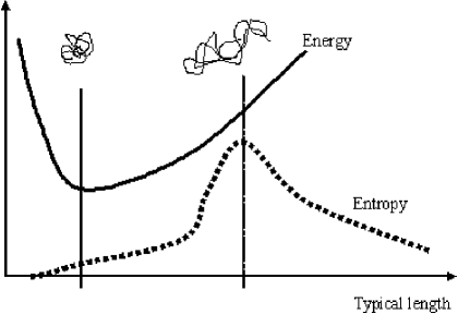
Figure 1: A sketch of the energy and entropy dependence on the linear size of a Methyl Cellulose polymer in water. The folded conformation costs less energy due to more favorable interactions between hydrophobic sequences along a single chain, but are less entropic as water molecules has to arrange in cage like structures around the hydrophobic constituents of the chain. The unfolded conformation admits much more microscopic configurations. The interaction with other polymers in the solution is suppressed in the folded state.

The main cause for inverse freezing is that the ”open” conformations of the polymer are also the interacting structures, as they allow for the formation of hydrophobic links with other polymers in the solution, a process that leads to gelation. This seems to be a general prescription to both inverse melting and inverse glass transitions: the noninteracting state is favored energetically, while the interacting state is favored by the entropy.

Let us now present a very simple model that incorporates these features. It is based on the Blume-Capel model Blume ,Capel for a spin one particle with ”lattice field” that lower the energy of the ”zero” (noninteracting) state. In contrast with the original Blume-Capel model, we consider the $\pm 1$ spin states (that interact with other spins) to be more degenerate. The system consists of a lattice of N sites and the Hamiltonian is given by

$$H=-J\sum_{<i,j>}S_{i}S_{j}+D\sum_{i=1}^{N}S_{i}^{2}$$ (1)

where the spin variables are allowed to assume the values $S_{i}=0,\pm 1$. The summation over $<i,j>$ is over each distinct pair once. Turning back to our polymer analogy, spin $0$ represents schematically the compact non-interacting polymer coil, the stretched polymer (interacting with its neighbors) is represented by spin $\pm 1$. The positive constant $D$ measures the energy preference of the compact spatial configurations, and the ”ferromagnetic” interaction between spins, $J$, is related to the concentration of polymers (or the pressure). The $0$ spin state is assumed to be n-fold degenerate, and the $\pm 1$ states are m-fold degenerate so that $r=m/n\geq 1$ is the degeneracy ratio that dictates the entropic advantage of the interacting states. It turns out that all the results presented here are independent of the absolute degeneracies $m$ and $n$, and depend only on their ratio $r$.

Using standard gaussian integral techniques one finds an expression for the free energy per spin in the infinite range limit:

$$f\equiv F/N=\beta Jm^{2}/2-ln[1+2\ r\ cosh(\beta Jm)e^{-\beta D}]$$ (2)

where m is the order parameter of the system (magnetization per spin), $m\equiv\langle\frac{1}{N}\sum_{i=1}^{N}S_{i}\rangle$. The phase transition curves are obtained numerically by solving for the minimum of Eq. (2) with respect to $m$. Scaling the temperature and $D$ with the interaction strength $J$, the phase diagram is shown in Figure (2). In the inset, results are presented for the original Blume-Capel model (i.e., the $r=1$ case): the line AB is a second order transition line, above it is a paramagnetic ($m=0$) phase and below it the system is Ferromagnetic ($m\neq 0$). Below the tricritical point (B) the phase transition is first order, and the three lines plotted are: the spinodal line of the ferromagnetic phase BE (above this line the $m\neq 0$ solution ceases to exist), the spinodal line of the paramagnetic phase BC (below this line there is no $m=0$ minimum of the free energy) and the first order transition line BD. Along BD the free energy of the paramagnetic phase is equal to that of the ferromagnetic state. Clearly, the Blume-Capel model displays no inverse melting: an increase of the temperature induces smaller order parameter.

The situation is different as $r$ increases, as emphasized by the main part of Figure (2). The same phase diagram is presented, but now $r=6$, so the interacting states have larger entropy. The tricritical point is shifted to the left, leaving a region of second order inverse melting, and the orientation of the BD line also changes, establishing the possibility of first order inverse melting. Note that the $r=6$ transition lines converge to the $r=1$ lines as $T\to 0$, since the entropy has no effect on the free energy at that limit. The ferromagnetic phase also covers larger area of the phase diagram for $r=6$, a fact that reflects again its entropic advantage.

Figure 2: Phase diagram and spinodal lines for the ordered model Eq. (2) in the $D-T$ plane for $r=1$ (Blume-Capel model, inset) and for $r=6$. The value of $r=6$ has been chosen in order for the effect to be more pronounced, but inverse melting is seen for $r$ lower than $2$

Figure 3: Phase diagram and the spinodal lines for the ordered Blume-Capel model in the interaction-temperature plane with $r=6$. The interaction J/D represents the concentration (”pressure”).

To allow qualitative comparison of our cartoon model with experimental results, the appropriate parameters should be identified. There are three parameters in the model as it stands: $D$ represents the energetic advantage of the noninteracting state, $r$ (if larger than 1) is the entropic gain of the interacting state, and $J$ is the strength of the interaction. In most of the physical systems that display inverse melting the controlled external parameter is the strength of the interaction: pressure (for $He^{3}$ and $He^{4}$) or concentration of the interacting objects (for polymeric systems and Rochelle salt - Ammonium Rochelle salt mixtures). As long as the only effect of the pressure is to increase the strength of the effective interaction among constituents, it may be modelled by changing $J$. The resulting phase diagram should be compared, though, with the $T-J$ plot of our model presented in Figure (3). The decrease of the transition temperature with the increase of interaction strength (pressure) is physically intuitive, as larger interaction favors energetically the ferromagnetic phase. As emphasized recently by stillinger , the slope of the first order transition line in the pressure-temperature plane is required by the corresponding Clausius-Clapeyron equation:

$$\frac{dP}{dT}=\frac{S_{2}-S_{1}}{V_{2}-V_{1}}$$ (3)

where $V_{2}$, $V_{1}$ are the volume (the extensive parameter conjugate to the pressure) of the solid and liquid phases respectively, and $S_{2}$, $S_{1}$ are their entropies. Inverse melting is possible if the numerator of (3) is negative, so for ”normal” transitions ($V_{2}>V_{1}$) one expects a negative slope of the transition line. In real magnetic or electric system the intensive-extensive pairs [magnetization-magnetic field ($\textbf{M}\cdot d\textbf{H}$) or polarization-electric field ($\textbf{P}\cdot d\textbf{E}$)], appear in the free energy function with inverse sign relative to $PdV$. If the order parameter vanishes, or takes smaller values, in the ”liquid” (disordered) phase, this implies also negative slope of the first order transition line in the temperature-external field plane. An interesting exception is the inverse melting of vortex liquid in superconductors, where the magnetization of the crystalline phase is smaller than that of the liquid and the transition line slope is actually positive.

Inverse freezing, the (reversible) appearance of glassy features in a system upon raising the temperature, may be incorporated in our model by introducing random coupling $J_{ij}$, as in the standard spin-glass models binder . This randomness may fit, in particular, to the gelation transition of Methyl Cellulose, as it occur only when the hydrophobic sequences are deposited at random along the chain. The random-exchange analogue of the Hamiltonian (1) is:

$$H=\sum_{<i,j>}J_{ij}S_{i}S_{j}+\sum_{i=1}^{N}DS_{i}^{2}$$ (4)

where the exchange interaction between the $i$ and the $j$ spin is taken at random from some predetermined distribution. Following the paradigmatic Sherrington-Kirkpatrick (SK) analysis binder of the infinite range spin glass, we assume gaussian distribution of the exchange term with zero mean:

$$P(J_{ij})=\sqrt{\frac{N}{2\pi\sigma^{2}}}\exp-(\frac{NJ_{ij}^{2}}{2J^{2}}),$$ (5)

where $\frac{J}{\sqrt{N}}$ is the width of the distribution. The replica trick is then implemented to get the free energy at the large $N$ limit.

The case $r=1$, namely the random exchange version of the Blume-Capel model, was first introduced and discussed by Ghatak and Sherrington (GS) Ghatak who used symmetric replica to obtain the relevant phase diagram. The GS solution seems to display inverse freezing even for the $r=1$ case, but more detailed analysis by da Costa et. al. Costa revealed that the glass order-parameter takes nonzero values (with a variety of stability features) in the area below the GS transition line, and the temperature dependence is monotonic. Recently, the full replica symmetry breaking analysis has been implemented for the GS model crisanti , and the results admit no inverse glass transition. Here we present a replica symmetric analysis of the same hamiltonian where the interacting states are highly degenerate, i.e., $r>1$. Following Costa , we obtain the phase transition and the spinodal lines, and the results support, again, both first and second order inverse glass transition.

The replica technique Edwards relies on the identity $\overline{ln[Z]}=lim_{n\rightarrow 0}\frac{1}{n}(\overline{Z^{n}}-1)$, where $Z$ is the partition function of the system and $Z^{n}$ is interpreted as the partition function of an n-fold replicated system $S_{i}\rightarrow S_{ia},a=1...n$. The average free energy may be computed using $\beta f=-lim_{n\rightarrow 0}\frac{1}{n}(\overline{Z^{n}}-1)$. The disorder average is taken for $Z^{n}$ using the Gaussian distribution (5) and gives:

$$\overline{Z^{n}}=Tr\exp\left[\frac{\beta^{2}J^{2}}{N}\sum_{a>b}(\sum_{i}S_{ia}S_{ib})^{2}+\right.$$

$$\left.\frac{\beta^{2}J^{2}}{2N}\sum_{a}(\sum_{i}S_{ia}^{2})^{2}-\beta D\sum_{i}S_{ia}^{2}\right]$$ (6)

where $a,b=1...n$ denotes the replica. Implementing the Hubbard-Stratanovitch identity yields the free energy per spin:

$$-\beta\frac{F}{N}=-\beta^{2}J^{2}\sum_{a>b}q_{ab}^{2}\ -\frac{\beta^{2}J^{2}}{2}\sum_{a}q_{aa}^{2}+lnTre^{\hat{L}}$$ (7)

where

$$\hat{L}=2\beta^{2}J^{2}\sum_{a>b}q_{ab}S_{a}S_{b}+\beta^{2}J^{2}\sum_{a}q_{aa}S_{a}^{2}-\beta D\sum_{a}S_{a}^{2}.$$

$q_{aa}$ and $q_{ab}$, the diagonal and the off diagonal entries of the ”order parameter matrix”, are given self-consistently by the saddle-point condition:

$$q_{ab} = \langle{S_{a}S_{b}}\rangle$$

$$q_{aa} = \langle{S_{a}^{2}}\rangle$$ (9)

where $\langle...\rangle$ stands for thermal average. In order to solve this model it is necessary to make assumptions on the order parameter matrix elements $q_{ab}$, and the simplest ansatz, is symmetry with respect to permutations of any pair of the replicas: $q_{ab}=q,\ \ \forall a\neq b$, $q_{aa}=p,\ \ \forall a$. Using this replica symmetric assumption one obtains

$$-\beta f = \frac{\beta^{2}J^{2}}{2}(q^{2}-p^{2})+\frac{1}{\sqrt{2\pi}}\int_{-\infty}^{\infty}dz\exp(-\frac{z^{2}}{2})\cdot$$ (10)

$$ln [1+2\ r\ e^{\gamma}\cosh(\beta J\sqrt{2q}z)$$

with

$$\gamma=\beta^{2}J^{2}(p-q)-\beta D$$ (11)

Extremizing the free energy with respect to q and p one gets by the following coupled equations:

$$q=\int_{-\infty}^{\infty}\frac{dz\ exp(-\frac{z^{2}}{2})}{\sqrt{2\pi}}\frac{4r^{2}e^{2\gamma}\sinh^{2}(\beta J\sqrt{2q}z)}{[1+2re^{\gamma}\cosh(\beta J\sqrt{2q}z)]^{2}}$$ (12)

$$p=\int_{-\infty}^{\infty}\frac{dz\ exp(-\frac{z^{2}}{2})}{\sqrt{2\pi}}\frac{2re^{\gamma}\cosh(\beta J\sqrt{2q}z)}{1+2re^{\gamma}\cosh(\beta J\sqrt{2q}z)}$$ (13)

The coupled equations (12) and (13) are numerically solved (with the possibility of multiple solutions if more than one stable state exists), and the location of the first order transition line is then determined by comparison of the free energy values (plugging $q$ and $p$ into (10)). The resulting phase diagram is shown in Fig. (4) for the case $r=6$, and displays all the essential features that exist in the ordered model, including a tricritical point and spinodal lines.

Figure 4: Phase diagram and the spinodal lines for the disordered model in the D-T plane for a constant interaction J for $r=6$.

To conclude, the basic theoretical insight of Blume and Capel, to have a spin model with low energy non-interacting (zero) state, may yield an inverse melting transition once the model is enriched with an entropic advantage of the interacting phase. It should be emphasized that the higher entropy associated with the interaction do not unavoidably entail inverse melting; this property may be ”buried” below energetic and other constraints that dominate the system, yet it may change the phase diagram predicted by the naive assumption that higher energy implies higher entropy.

The authors wish to acknowledge Prof. Y. Rabin for most helpful discussions of the subject.

References

- (1) E.R. Dobbs, Helium Three, Oxford University press, Oxford UK (2002). C. La Pair et. al., Physica 29, 755 (1963).
- (2) S. Rastogi, G. W. H. Hohne, and A. Keller, Macromolecules 32, 8897 (1999); A. L. Greer, Nature 404, 134 (2000).
- (3) See, e.g., C. Kittel, Introduction to solid state physics (John Wiley, NY 1966) chapter 13. T. Mitsui, Phys. Rev. 111, 1259 (1958). U. Schneider, P. Lunkenheimer, J. Hemberger and A. Loidl, Ferroelectrics 242 , 71 (2000).
- (4) D. Ertas and D. R. Nelson, Physica C 272, 79 (1996); N. Avraham, B. Khaykovich, Y. Myasoedov, M. Rappaport, H. Shtrikman, D. E. Feldman, T. Tamegai, P. H. Kes. M. Li, M. Konczykowski, K. van der Beek, and E. Zeldov, Nature,411, 451 (2001).
- (5) C. Chevillard, M. Axelos, Colloid. Polym. sci.,275, 537,(1997); J. Desbrieres, M.A.V. Axelos and M. Rinaudo, Polymer 39, 6251 (1998).
- (6) S. Z. Ren and C. M. Sorensen, Phys. Rev. Lett. 70, 1727 (1993).
- (7) A. K. Chakraborty and E.I. Shakhnovich, J. Chem. Phys. 103, 10751 (1995); D. Bratko, A. K. Chakraborty and E.I. Shakhnovich,J. Chem. Phys. 106, 1264 (1997).
- (8) O. Mishima and H. G. Stanley, Nature 396, 329 (1998).
- (9) Haque A. and Morris E., Carbohydrates Polymers 22, 161 (1993).
- (10) M. Blume, Phys. Rev. 141, 517 (1966).
- (11) Physica (Utr.) 32, 966 (1966), Physica 33, 295 (1967), Physica 37, 423 (1967).
- (12) F. H. Stillinger and P. G. Debenedetti, Biophysical Chemistry 105, 211 (2003).
- (13) See, e.g., Binder K. and Young A. P., Rev. Mod. Phys. 58, 801 (1985) and references therein.
- (14) S. K. Ghatak and D. Sherrington, J. Phys. C: Solid State Phys. 10, 3149 (1997).
- (15) P. J. Mottishaw and D. Sherrington, J. Phys. C: Solid State Phys. 18, 5201, (1985).
- (16) E. J. S. Lage and J. R. L. Almeida, J. Phys. C.: Solid State Phys. 15, L1187 (1982).
- (17) A. Crisanti and L. Leuzzi, Phys. Rev. Lett. 89, 237204 (2002).
- (18) F. A. da Costa, C. S. O. Yokoi, and S. R. A. Salinas, J. Phys. A: 27, 3365 (1994);
- (19) S. F. Edwards and P. W. Anderson, J. Phys. F: Met. Phys. 5, 965-974 (1975).