Application of detrended fluctuation analysis to monthly average of the maximum daily temperatures to resolve different climates

Abstract

Detrended fluctuation analysis is used to investigate correlations between the monthly average of the maximum daily temperatures for different locations in the continental US and the different climates these locations have. When we plot the scaling exponents obtained from the detrended fluctuation analysis versus the standard deviation of the temperature fluctuations we observe crowding of data points belonging to the same climates. Thus, we conclude that by observing the long-time trends in the fluctuations of temperature it would be possible to distinguish between different climates.

I INTRODUCTION

Ever since it was first realized that humanity is capable of changing its natural surroundings more rapidly than nature can repair it, model-based predictions about climate change has been one of the main research areas in science. While many climatologists firmly believe that there is strong evidence for our interference in nature in general and in climate in particular, a few others disagree.

Before we can even attempt to settle this debate, there are quite a few questions that we need to answer about the climate of the past. Nature provides us with different forms of data which we can convert to climatic data. For datasets reflecting the near past, it is rather simple to obtain information about the climate as we can always rely on the recorded history. For example, tree ring history from Scandinavia indicates that there was a period of high temperatures between 9th and 13th centuries, called the ”Medieval Warm Period” Cook13050 . The tree ring temperature history for this period agrees with the glacier data, and has been supported by the historical records of Norse seafaring and colonization around the North Atlantic at the end of the 9th century. It is known that during this time the warmer climate helped in producing greater harvests in Iceland and parts of Greenland Bryson13060 which in turn helped the colonies in Greenland. But when we go to older times, it becomes more and more difficult to relate the paleoclimatic proxies to the climate of a certain region. From paleoclimatic proxies, like tree ring indices or stacked oxygen-isotope curves derived from deep sea cores, we normally obtain fluctuations of the local temperatures rather than their absolute values. Therefore, it is difficult to construct a method to characterize different climates based solely on the fluctuations of temperature values.

The weather forecast to first approximation, is a rather simple issue. A cold day is usually followed by a cold day, and a warm day is usually followed by a warm day. On a larger scale, a colder week is usually followed by a warmer week which corresponds to the average duration of the general weather regimes. But as the longer timescales are governed by different processes like circulation patterns and sometimes even influenced by trends like global warming, defining long-term correlations becomes more difficult.

In order to separate the trends and the correlations we need to eliminate the trends in our temperature data. Several methods are used effectively for this purpose: rescaled range analysis (R/S) Mandelbrot12180 ; Mandelbrot12190 ; Bodri13500 ; Bodri13530 , wavelet techniques (WT) Arneodo5250 ; Koscielny-Bunde13240 and detrended fluctuation analysis (DFA) Peng13540 ; Koscielny-Bunde13250 .

Analysis of the temperature fluctuations over a period of decades on different parts of the globe has already showed the effectiveness of the application of detrended fluctuation analysis to characterize the persistence of weather and climate regimes. DFA and WT have been applied to study temperature and precipitation correlations in different climatic zones on the continents and also in the sea surface temperature of the oceans. The recent results show that the temperatures are long range power-law correlated. The long-term persistence of the temperatures can be characterized by an auto-correlation function $C(n)$ of temperature variations where $n$ is the time between the observations. The auto-correlation function decays as $C(n)\sim n^{-\gamma}$. Even though there is some disagreement on the value of the exponent $\gamma$, the fact that the persistence of the temperatures can be characterized by this auto-correlation function is firmly established. Different groups have used R/S, DFA and WT analysis and have shown that this exponent $\gamma$ has roughly the same value $\gamma\simeq 0.7$ for the continental stations Bodri13500 ; Bodri13530 ; Koscielny-Bunde13250 ; Bunde13180 ; Kantelhardt13220 ; Eichner13120 ; Weber2830 ; Talkner3550 . The exponent $\gamma$ is found to be roughly 0.4 for island stations Bunde13180 ; Eichner13120 and sea surface temperature on the oceans Bunde13180 ; Monetti13140 . This method has also been applied to the temperature predictions of coupled atmosphere-ocean general circulation models Bunde100 ; Govindan13190 ; Blender13260 ; Fraedrich13270 ; Fraedrich12720 but there is disagreement on the actual value of the exponent $\gamma$. On one side it is argued that the exponent does not change with the distance from the oceans Bunde100 ; Eichner13120 and is roughly $\gamma\simeq 0.7$. On the other side it is said that the scaling exponent is roughly 1 over the oceans, roughly 0.5 over the inner continents and about 0.65 in transition regions Blender13260 ; Fraedrich13270 ; Fraedrich12720 .

Previous work in this area also shows that there is a slight variation in the scaling exponent between the low-elevation, mountain, continental and maritime stations Weber2830 ; Talkner3550 . Even though these variations are between $\gamma\simeq 0.5$ and $\gamma\simeq 0.7$ the fact that they show a correlation with location and elevation indicates that a relationship between the statistical nature of the temperature fluctuations and the climate can be established.

II METHOD

Daily temperature data have a non-stationary nature due to seasonal trends. To remove this seasonal trend effect, the mean temperature for each day over all the years in the data set is determined. Subsequently, mean daily maximum temperature was obtained by calculating the fluctuation from the mean daily maximum temperature,

$$\Delta T_{i}=T_{i}-<T_{i}>$$ (1)

where $<T_{i}>$ is the mean daily maximum temperature. Similarly we can also use the mean daily average temperature or the mean daily minimum temperature, and the use of average or minimum temperature instead of maximum temperatures does not change the outcome of the analysis Talkner3550 . To remove the remaining linear trends (the average temperature for some years can be higher or lower than the average temperature of the time series for that location as a result of atmospheric processes), we applied DFA Peng13540 , which essentially enables us to investigate long-term correlations in the data by getting rid of the trends.

The standard calculation of the autocorrelation function is hindered by the noise and nonstationarity in the data. Instead of calculating $C(n)$ directly and reducing the noise in the time series, a running sum of the temperature fluctuations is considered,

$$y(m)=\sum_{i=1}^{n}\Delta T_{i}$$ (2)

where $m=1,,N$. $N$ is the length of the time series in question. The fluctuations in this sum are related to $C(n)$ by

$$\overline{F(n)^{2}}\sim n^{2\alpha}$$ (3)

Next, the time series of the $y(m)$ is divided into non-overlapping intervals of equal length $n$. In each interval, we fit $y(m)$ to a straight line ($x(m)=km+d$ for each segment) and calculate the detrended square variability $\overline{F(n)^{2}}$ as

$$\overline{F^{2}(n)}=<\frac{1}{n}\sum_{m=kn+1}^{(k+1)n}(y(m)-x(m))^{2}>$$ (4)

with

$$k=0,1,2,...,(\frac{N}{n}-1).$$ (5)

If the temperature fluctuations were uncorrelated (i.e. white noise) we would expect

$$F(n)\sim n^{\alpha}$$ (6)

with $\alpha=\frac{1}{2}$. If $\alpha>\frac{1}{2}$, we expect long-range power law correlations in the data for the range of values considered.

Figure 1 shows $F(n)$ for one US station as an arbitrary example (all other stations in our dataset, where daily temperature data is available, show similar behavior). For this station, (Millinocket, Maine) we have plotted the $F(n)$ for both daily and monthly temperature data. To calculate the monthly temperature data we took the average of the maximum daily temperatures for each month and used DFA on the monthly averages. Figure 1 shows that for a time period longer than about 60 days, both the daily and monthly temperature data give us the same scaling exponent $\alpha$. This behavior has been observed before for daily temperature data Weber2830 ; Talkner3550 . As the results of our analysis for daily and monthly data at all the sampled locations agrees for long time scales ($n>$ 60 days) the results presented in this paper have been obtained from the analysis of monthly averages. Both the daily ($n>$ 60 days) and monthly averages span about two decades, indicating correlations of 30 years or more. We are aware of the fact that by taking the monthly averages we are effectively losing information about the dataset, i.e. about correlations at a short time scale. However, as our main interest is in finding correlations in the longer time scales, in the light of the information obtained from Figure 1, we believe that this loss does not change the behavior of these data at longer time scales. In addition, much wider and reliable availability of monthly averages lead us to sacrifice short time scales for the sake of obtaining longer time series of data.

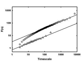
Figure 1: Detrended variability $F(n)$ is plotted against a timescale. The circles represent daily maximum temperatures, the triangles represent monthly average temperatures. The slope of both of the curves gives $\alpha=0.53\pm 0.03$ (the slope for the daily maximum temperatures is calculated for the time period longer than 60 days). Data belongs to station, Millinocket, Maine.

In the present work we have investigated temperature fluctuations for 129 weather stations in the continental US. The data has been obtained from the U.S. Historical Climatology Network US13720 . From the available data we have chosen the stations with the longest records. We did not include in our analysis datasets with data shorter than 75 years, and the longest dataset we had spanned 110 years at several locations in the dataset (all ending in 1994). The data come from the coastal regions of California (14 stations), Alabama (15 stations), Maine (12 stations), New Mexico (24 stations), West Virginia (13 stations), Michigan (17 stations), Montana (14 stations), and Arizona (20 stations).

For these 129 continental U. S. stations the value of the exponent is found to be $\alpha=0.60\pm 0.05$. The individual error bars for the data points have been of the order of $\Delta\alpha\simeq 0.01$. Figure 2 gives a summary of the scaling exponents obtained from these 129 stations. As we can see from this figure, consistent with the earlier observations Eichner13120 ; Govindan13190 ; Koscielny-Bunde13240 ; Koscielny-Bunde13250 we obtain scaling exponents in the range of 0.52 to 0.72. The scaling exponents for the eight different states are coastal California ($\alpha=0.63\pm 0.06$), Alabama ($\alpha=0.56\pm 0.03$), Maine ($\alpha=0.60\pm 0.04$), West Virginia ($\alpha=0.56\pm 0.02$), New Mexico ($\alpha=0.64\pm 0.04$), Arizona ($\alpha=0.61\pm 0.03$), Michigan ($\alpha=0.58\pm 0.02$), and Montana ($\alpha=0.58\pm 0.02$) respectively.

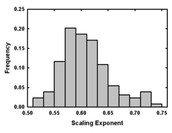
Figure 2: The histogram of the scaling exponents. The average from the 120 station gives a scaling exponent of $\alpha=0.60\pm 0.05$.

It has been suggested that the value of the exponent $\alpha$ depends on the geographic location (distance from the oceans Fraedrich13270 and elevation Weber2830 ). To investigate this effect of location on the exponent $\alpha$ we first looked at the correlations between the elevation of the weather stations and the resulting exponent $\alpha$ in Figure 3. It is very difficult to observe any trends in the data with changing elevation as most of the correlations are within one standard deviation. We might say that at elevations of about 200 meters (the stations at 100-250 meters give an exponent $\alpha=0.57\pm 0.03$, the scaling exponent is slightly lower than the coastline (the stations at 0-100 meters give an exponent $\alpha=0.62\pm 0.05$). Above the elevation of 250 meters the scaling exponent increases slightly with elevation.

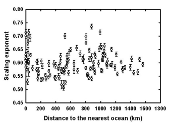
Figure 3: The dependence of the scaling exponent on the elevation of the weather station.

Previous work suggested that the scaling exponent changed from 1 over the oceans to 0.5 over the inner continents. The coastal regions appeared as transition regions corresponding to a scaling exponent of about 0.65 Fraedrich13270 . Figure 4 shows the relation between the distance between the station and nearest ocean, and the scaling exponent. We observe no change in the scaling exponent for the inner continental stations, which contradicts the previous work, but the distance of the observational station previously used, was about 2000 kms from any ocean, whereas in our data set, the largest distance between any of the stations and the nearest ocean is about 1600 kms. Therefore we cannot comment on the possibility that the exponent changes to smaller values for even more ”inner continental” stations. Latest work also agrees with our data in showing no change with increasing distance from the coastline Eichner13120 .

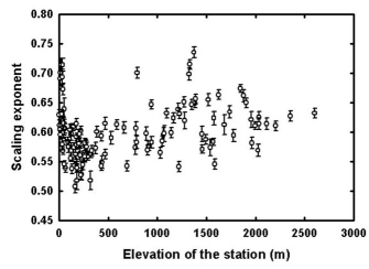
Figure 4: The dependence of the scaling exponent on the distance of the weather station from the nearest coastline (ocean).

When we look at the scaling exponents and consider only the geographic locations of the stations it is almost impossible to distinguish these states from each other unambiguously. However a striking result can be observed if we plot the standard deviation of the temperature fluctuations versus the scaling exponent observed from that station. These standard deviations of the temperature fluctuations are calculated over the whole dataset where each point consists of a monthly average of daily maximum temperatures. It is known that the standard deviation is a correct measure of fluctuations only if the underlying distribution is a pure Gaussian, and daily and monthly temperatures are known to show skewed distributions. The coefficient of skewness is defined as Press13730

$$Skewness(x_{1}...x_{N})=\frac{1}{n}\sum_{j=1}^{N}[\frac{x_{j}-\overline{x}}{\sigma}]^{3}$$ (7)

where $\sigma=\sigma(x_{1}...x_{N})$ is the distribution’s standard deviation. A positive value of skewness signifies a distribution where an asymmetric tail extends out towards more positive $x$ values and a negative value of skewness gives a distribution with an asymmetric tail extending out towards more negative $x$ values. For the idealized case of a Gaussian distribution, the standard deviation of the coefficient of skewness is approximately $\sqrt{6/N}$. In real life it is a good practice to account for skewnesses only if the coefficient of skewness obtained from the distribution is many times larger than this value Press13730 . We have randomly chosen five of the stations to test for skewness. For all of these stations the period of the time series was 102 years. For comparison the standard deviation of the coefficient of skewness for a Gaussian distribution is $\sqrt{6/1224}=0.07$. The coefficients of skewness for these stations are 0.03 (Brewton, AL), 0.09 (Berkeley, CA), -0.05 (Crow Agency, MT), -0.04 (State University, NM), and -0.06 (Glenville, WV). Figure 5 shows the frequency of the deviations from the monthly average temperatures for a sample station, Glenville, WV. As a side note, we have performed the same skewness analysis for these stations using the average monthly maximum temperatures instead of the deviation from the average maximum temperatures. The skewness of this data was significantly higher justifying the point that climatic data itself can have a strongly skewed distribution (-0.17 (Brewton, AL), -0.28 (Berkeley, CA), -0.13 (Crow Agency, MT), -0.17 (State University, NM), and -0.20 (Glenville, WV)). Therefore we decided that the standard deviation of temperature fluctuations from the average temperatures can be used in statistical description of a dataset as long as the climate does not change during that given period of time.

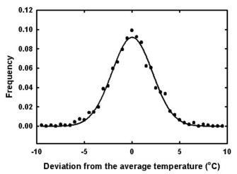
Figure 5: The frequency of the deviation of the monthly temperatures from the monthly average temperatures. The fitting line is to a Gaussian distribution.

We are aware that state or country boundaries are not good indicators for identifying different regions, however, within many small states or countries, the climate does not change significantly. In cases where the climate is different in different parts of the state, we have either ignored the data from those stations, or just analyzed one part of the state as in the case of coastal California. Therefore, we can safely assume that the climates in these states can be classified as Humid Subtropical - Mediterranean (Coastal California), Humid Subtropical - East Coasts (Alabama), Humid Continental - Hot Summers - Year around precipitation (West Virginia), Humid Continental - Mild Summers - Year around precipitation (Maine) and Dry/Arid - Hot - Low Latitude desert (New Mexico).

Figures 6-10 give the scaling exponent for coastal California, Alabama, Maine, West Virginia, and New Mexico versus the standard deviation of the temperature fluctuations, respectively. In these figures we can identify that the scaling exponents crowd different regions of the graph indicating a possibility that these different climates can be distinguished from each other using the method described above. We must be clear about one point: If we have only the standard deviations of the temperature fluctuations and the scaling exponents resulting from those distributions, obtaining clusters which would indicate different climates, is extremely difficult. However the question we are trying to answer is simpler: We know where the stations are located (on the standard deviation of temperature fluctuations versus the scaling exponents map) for Humid Subtropical - Mediterranean climate. Can we now identify an unknown station as having a Humid Subtropical - Mediterranean climate? To be able to answer this question we have used the support vector machine (SVM) algorithm Vapnik13740 for data classification.

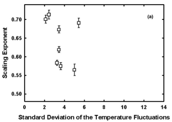
Figure 6: The scaling exponents plotted against the standard deviation of the temperature fluctuations for coastal California.

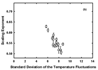
Figure 7: The scaling exponents plotted against the standard deviation of the temperature fluctuations for Alabama.

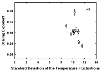
Figure 8: The scaling exponents plotted against the standard deviation of the temperature fluctuations for Maine.

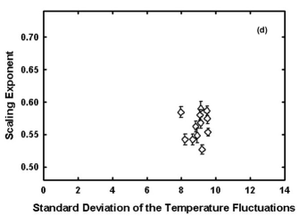
Figure 9: The scaling exponents plotted against the standard deviation of the temperature fluctuations for West Virginia.

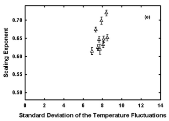
Figure 10: The scaling exponents plotted against the standard deviation of the temperature fluctuations for New Mexico.

A data classification task normally uses training and testing data. Each instance in the training data set consists of one target value (in our case belonging to a specific climate type) and several features (like the standard deviation of the temperature fluctuations and the scaling exponent). The aim of SVM Joachims13750 is to produce a model which then predicts the target value of data instances in the testing set. In training set we have used 10 positive target values (belonging to the climate class we are analyzing) and 20 negative target points (belonging to different climate classes). In the testing set, we supplied the algorithm with all of the stations in our data set and asked the program to identify the different regions. The performance of such an algorithm is usually quantified by its accuracy during the test phase which mainly depends on the correct treatment of true positives (TP) and true negatives (TN). It is usually also important to distinguish between two types of errors: A false positive (FP) and a false negative (FN). Consequently, the performance of the prediction is better judged if we add two more quantifiers, sensitivity and specificity. The accuracy of the data classification is defined as the ratio between the number of correctly identified samples and the total number of samples:

$$accuracy=\frac{TP+TN}{TP+FP+TN+FN}$$ (8)

The sensitivity is the ratio between the number of true positive predictions and the number of positive instances in the test set:

$$sensitivity=\frac{TP}{TP+FN}$$ (9)

Finally, the specificity is defined as the ratio between the number of true negative predictions and the number of negative instances in the test set:

$$specificity=\frac{TN}{FP+TN}$$ (10)

For our initial analysis, we used only the five different climates mentioned above. The results are summarized in Table 1. Considering that we have a test set of 78 stations the deviations from $100\%$ for any of the accuracy, sensitivity, and specificity values are caused by at most 4 stations identified either as false positives or false negatives. We believe that this small discrepancy is caused by microclimatic behavior for those stations. For example, the only false positive for Humid Subtropical - Mediterranean climate comes from the only coastal station in Alabama.

Table 1: SVM analysis of the 78 weather stations in 5 different climate zones. Accuracy, sensitivity, and specificity are defined in the text.

Climate Type	Accuracy	Sensitivity	Specificity
Humid Subtropical - Mediterranean (Coastal California)	$98.7\%$	$100.0\%$	$98.4\%$
Humid Subtropical - East Coasts (Alabama)	$96.2\%$	$100.0\%$	$95.2\%$
Humid Continental - Mild Summers - Year around precipitation (Maine)	$98.7\%$	$91.7\%$	$100.0\%$
Dry/Arid - Hot - Low Latitude desert (New Mexico)	$96.2\%$	$100.0\%$	$94.4\%$
Humid Continental - Hot Summers - Year around precipitation (West Virginia)	$94.9\%$	$100.0\%$	$93.9\%$

To test this method even further, we have used SVM algorithm on the remaining 51 stations. Out of these 51 stations, 31 were in Montana and Michigan (Humid Continental - Mild Summers - Year around precipitation climate like Maine) and 20 were in Arizona (Dry/Arid - Hot - Low Latitude desert climate like New Mexico). Montana and Michigan are geographically different from Maine both in distance from the coastline and elevation. Arizona is geographically similar to New Mexico in distance from the coastline and elevation. In the analysis, we have treated Maine as our known climate, and together with the other states, Montana and Michigan as our ”unknowns”. Table 2 shows the results of this analysis. As expected, accuracy, sensitivity and specificity dropped slightly when we considered significantly different geographic locations. However, we still have more than 95predicting the climate of Michigan and Montana based solely on this analysis. In the second part of this analysis, we have considered New Mexico as our known climate, and together with the other states in our dataset, Arizona as our ”known” climate. The results show that all of the stations in Arizona are correctly identified as belonging to Dry/Arid - Hot - Low Latitude desert climate except for one station. Improvement in the statistics is caused by increasing the number of stations.

Table 2: SVM analysis of the whole data set in 2 different climate zones. For Humid Continental climate, the weather stations in Maine are taken as ”known” and data classification is performed to see whether the weather stations in Montana and Michigan are picked out as well for this climate. Similar analysis is done for the New Mexico and Arizona pair.

Climate Type	Accuracy	Sensitivity	Specificity
Humid Continental - Mild Summers - Year around precipitation (Maine)	$95.4\%$	$90.7\%$	$97.7\%$
Dry/Arid - Hot - Low Latitude desert (New Mexico)	$96.9\%$	$97.7\%$	$96.5\%$

III CONCLUSION

In this study, the variability of the weather in different parts of the continental US, as an example of different climates, has been investigated. Our results suggest that different climates can be readily distinguished using the detrended fluctuation analysis method on the fluctuations of the maximum daily temperatures. Even though we have used state boundaries to define the climates, as long as a mild, subtropical, Mediterranean climate exists in Coastal California, this method should be equally applicable to distinguish this climate from New Mexico where a dry, arid, hot desert climate is observed.

The results presented here are preliminary, based on stations with known climates. The real challenge lays in the future ability of this method to be applied to paleoclimatic data to reveal structure over timescales not only of the order of decades but that of millions of years. This point stays speculative as no reliable monthly data exists beyond 218 years Koscielny-Bunde13240 (to our knowledge). However, the fact that this data does not seem to scatter appreciably at longer timescales Monetti13140 gives us hope about expanding the use of the method mentioned above.

- (1) R. Cook, Climate Dynamics 11, 211 (1995).
- (2) E. R. Bryson and T.J. Murray, Climates of Hunger (University of Wisconsin Press, Madison, 1977).
- (3) B. B. Mandelbrot, J. R. Wallis, Water Resources Research 5, 321 (1969).
- (4) B. B. Mandelbrot, J. R. Wallis, Water Resources Research 5, 967 (1969).
- (5) L. Bodri, Theoretical and Applied Climatology 51, 51 (1995).
- (6) L. Bodri, Theoretical and Applied Climatology 49, 53 (1994).
- (7) A. Arneodo, E. Bacry, P. V. Graves, J. F. Muzy, Phys. Rev. Lett. 74, 3293 (1995).
- (8) E. Koscielny-Bunde, A. Bunde, S. Havlin, H. E. Roman, Y. Goldreich, H. J. Schnellnhuber, Phys. Rev. Lett. 81, 729 (1998).
- (9) C. K. Peng, S. V. Buldyrev, S. Havlin, M. Simmons, H. E. Stanley, A. L. Goldberger, Phys. Rev. E 49, 1685 (1994).
- (10) E. Koscielny-Bunde, A. Bunde, S. Havlin, Y. Goldreich, Physica A 231, 393 (1996).
- (11) A. Bunde, S. Havlin, Physica A 314, 15 (2002).
- (12) J. W. Kantelhardt, E. Koscielny-Bunde, H. H. A. Rego, S. Havlin, A. Bunde, Physica A 295, 441 (2001).
- (13) J. Eichner, E. Koscielny-Bunde, A. Bunde, S. Havlin, H. J. Schnellnhuber, Phys. Rev. E 68, 046133 (2003).
- (14) R. O. Weber, P. Talkner, J. Geophys. Res. Atmos. 106, 20131 (2001).
- (15) P. Talkner, R. O. Weber, Phys. Rev. E 62, 150 (2000).
- (16) R. A. Monetti, S. Havlin, A. Bunde, Physica A 320, 581 (2003).
- (17) A. Bunde, J. Eichner, R. Govindan, S. Havlin, E. Koscielny-Bunde, D. Rybski, D. Vjushin, Preprint, physics/0208019 (2003).
- (18) R. Govindan, D. Vjushin, A. Bunde, S. Brenner, Y. Ashkenazy, S. Havlin, H. J. Schnellnhuber, Phys. Rev. Lett. 89, 028501 (2002).
- (19) R. Blender, K. Fraedrich, Geophys. Res. Lett. 30, 1769 (2003).
- (20) K. Fraedrich, R. Blender, Phys. Rev. Lett. 90, 108501 (2003).
- (21) K. Fraedrich, R. Blender, Phys. Rev. Lett. 92, 039802 (2004).
- (22) U.S. Hist. Climat. Network, http:// cdiac.esd.ornl.gov/ epubs/ ndp019/ statemax.html.
- (23) W.H. Press B.P. Flannery, S.A. Teulkovsky, W.T. Vetterling, Numerical Recipes in C: The Art of Scientific Computing (Cambridge University Press, 1992).
- (24) V.N. Vapnik The Nature of Statistical Learning Theory (Springer Verlag, 1995).
- (25) T. Joachims Advances in Kernel Methods - Support Vector Learning (M.I.T. Press, 1999).