Exact Results for Spectra of Overdamped Brownian Motion in Fixed and Randomly Switching Potentials

Abstract

The exact formulae for spectra of equilibrium diffusion in a fixed bistable piecewise linear potential and in a randomly flipping monostable potential are derived. Our results are valid for arbitrary intensity of driving white Gaussian noise and arbitrary parameters of potential profiles. We find: (i) an exponentially rapid narrowing of the spectrum with increasing height of the potential barrier, for fixed bistable potential; (ii) a nonlinear phenomenon, which manifests in the narrowing of the spectrum with increasing mean rate of flippings, and (iii) a nonmonotonic behaviour of the spectrum at zero frequency, as a function of the mean rate of switchings, for randomly switching potential. The last feature is a new characterization of resonant activation phenomenon.

05.40-a, 05.10.Gg, 02.50.Ga

1 Introduction

Spectral densities of fluctuations provide an important tool to characterize physical systems, because they can be measured directly in experiments. The investigations of spectra are useful to observe and analyze the interplay between fluctuations, relaxation and nonlinearity which are inherent to real physical systems. This interplay ranks among the most challenging problems of modern nonlinear physics and forms the basis of well-known nonlinear phenomena like stochastic resonance [1], resonant activation [2], noise-enhanced stability [3, 4], ratchet-effect [5, 6], etc.
The exact formulae for spectra of fluctuations in nonlinear dynamical systems were first derived for thermal diffusion in fixed potentials. Caughey and Dienes [7] pioneered in applying analytical method based on Laplace transform of conditional probability density to the first-order system with $V$-shaped potential. Another approach has its origins in the expansion of probability density of transitions in terms of Fokker-Planck kinetic operator eigenfunctions. This method was applied in [8] for obtaining correlation function of a bistable system with rectangular potential profile. We would also mention theoretical and numerical calculations reported in refs. [9], concerning the spectra of underdamped double-well system driven by white Gaussian noise. In these papers the spectral peaks corresponding to standard resonance and transitions between steady states have been revealed. Stationary spectra of fluctuations for monostable and bistable potential profiles, by analog simulations of underdamped stochastic system driven by colored noise, have been experimentally obtained in ref. [10]. The model of one-dimensional Brownian motion in singular potential like the potential of hydrogen atom was investigated in [11]. Authors detected some region of power spectrum with $1/f$ frequency dependence.
Despite a lot of work has been done to analyze spectra of fluctuations in the presence of one noise source, there is however lack of investigation on the so-called two-noise system spectra of fluctuations. A paradigmatic model is the overdamped Brownian motion in a randomly fluctuating potential. This model is being studied intensively in view of wide application in physics, chemistry and biology. However, an exact analytical results have been obtained only for escape rates, as mean first-passage times and lifetimes [4, 12] and stationary probability distributions of Brownian motion [13]. In this paper we report the exact calculations of diffusion spectrum for Brownian particle moving in fixed double-well potential and dichotomously switching linear potential. Our theoretical results, based on Markovian theory and on Laplace transform of conditional probability density, are valid for arbitrary intensity of driving white Gaussian noise and arbitrary parameters of potential profiles. We find: (i) a narrowing of the spectrum with increasing height of the potential barrier for fixed potential; (ii) a narrowing of the spectrum with increasing mean rate of flippings, and (iii) a nonmonotonic behaviour of the spectrum at zero frequency, as a function of the mean rate of switchings, for randomly switching potential. This last behaviour is a new characterization of resonant activation phenomenon [2].

2 Basic equations

Let us consider an overdamped Brownian motion in a fixed potential $U(x)$ described by Langevin equation

$$\frac{dx}{dt}=-\frac{dU\left(x\right)}{dx}+\xi\left(t\right),$$ (1)

where $x(t)$ is the position of Brownian particle, $\xi(t)$ is a $\delta$-correlated Gaussian noise with zero mean and intensity $2D$. The Fokker-Planck equation, or Smoluchowski equation [14], for the conditional probability density $W(x,t\left|x_{0},0\right.)$ of Markovian random process $x(t)$, corresponding to (1), is

$$\frac{\partial W}{\partial t}=\frac{\partial}{\partial x}\left[\frac{dU\left(x\right)}{dx}W\right]+D\frac{\partial^{2}W}{\partial x^{2}}$$ (2)

with initial condition

$$W(x,0\left|x_{0},0\right.)=\delta\left(x-x_{0}\right).$$ (3)

Let us assume that a stationary regime exists, then the probabilistic flow equals zero at $x\rightarrow\pm\infty$

$$\left[D\frac{\partial W}{\partial x}+U^{\prime}\left(x\right)W\right]_{x=\pm\infty}=0.$$ (4)

The correlation function of Brownian particle displacement $x(t)$ in a stationary state can be calculated as [15]

$$K\left[\tau\right]=\int\limits_{-\infty}^{+\infty}x_{0}W_{\infty}\left(x_{0}\right)dx_{0}\int\limits_{-\infty}^{+\infty}xW(x,\tau\left|x_{0},0\right.)dx,$$ (5)

where $W_{\infty}(x)$ is the stationary probability density (SPD) [14, 16]

$$W_{\infty}\left(x\right)=C\cdot\e^{-U\left(x\right)/D},\qquad C=\left[\int\limits_{-\infty}^{+\infty}\e^{-U\left(x\right)/D}dx\right]^{-1}.$$ (6)

To obtain the correlation function $K\left[\tau\right]$ we need to solve the second-order partial differential equation (2) using eigenfunction expansion [8, 14]. However, as shown in [7, 15], the determination of SPD (6) together with the Laplace transform method are sufficient for calculating the spectral density. In fact from Wiener-Khinchin theorem we have

$$S\left(\omega\right)=\frac{1}{2\pi}\int\limits_{-\infty}^{+\infty}K\left[\tau\right]\cos\left(\omega\tau\right)d\tau=\frac{1}{\pi}\mathrm{Re}\left\{\tilde{K}\left[i\omega\right]\right\},$$ (7)

where $\tilde{K}\left[p\right]$ is Laplace transform of $K\left[\tau\right]$. By Laplace transforming (2), with initial condition (3), we obtain

$$D\frac{d^{2}Y}{dx^{2}}+\frac{d}{dx}\left[U^{\prime}\left(x\right)Y\right]-pY=-\delta\left(x-x_{0}\right),$$ (8)

a second-order ordinary differential equation, where $Y\left(x,x_{0},p\right)$ is the Laplace transform of conditional probability density

$$Y\left(x,x_{0},p\right)=\int\limits_{0}^{+\infty}\e^{-pt}W(x,t\left|x_{0},0\right.)dt.$$ (9)

According to Eqs. (4) and (9) we solve (8) with boundary conditions

$$\left[D\frac{dY}{dx}+U^{\prime}\left(x\right)Y\right]_{x=\pm\infty}=0.$$ (10)

By using Eqs. (5) and (9) the Laplace transform $\tilde{K}\left[p\right]$ of the correlation function is

$$\tilde{K}\left[p\right]=\int\limits_{-\infty}^{+\infty}x_{0}W_{\infty}\left(x_{0}\right)dx_{0}\int\limits_{-\infty}^{+\infty}xY\left(x,x_{0},p\right)dx.$$ (11)

Then, after substitution of $p=i\omega$ in (11) we can find the spectral density $S(\omega)$ from (7). Thus for calculating spectrum it will suffice to solve ordinary differential equation (8) and make double integration, instead of solving partial differential equation (2). To end we need the explicit expression of the internal integral in (11). By multiplying both parts of (8) on $x$ and integrating it over the total area, using boundary conditions (10), we obtain

$$G\left(x_{0},p\right)\equiv\int\limits_{-\infty}^{+\infty}xY\left(x,x_{0},p\right)dx=\frac{x_{0}}{p}-\frac{D}{p}\left[Y\left(\infty,x_{0},p\right)-Y\left(-\infty,x_{0},p\right)\right]$$

$$-\frac{1}{p}\int\limits_{-\infty}^{+\infty}U^{\prime}\left(x\right)Y\left(x,x_{0},p\right)dx.$$ (12)

3 Fixed bistable potential

Let us calculate the spectral density for symmetric double-well piecewise linear potential (see Fig. 1)

$$U(x)=\left\{\begin{array}[c]{cc}E\left(1-\left|x\right|\left/L\right.\right),&\left|x\right|\leq L,\\ +\infty,&\left|x\right|>L.\end{array}\right.$$ (13)

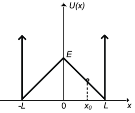
Figure 1: Double-well piecewise linear potential.

Substituting (13) in (8),(10) we obtain the following equation for the Laplace transform $Y(x,x_{0},p)$ of conditional probability density

$$DY^{\prime\prime}-\frac{E}{L}\left[\mathrm{sgn}\left(x\right)Y\right]^{\prime}-pY=-\delta\left(x-x_{0}\right)$$ (14)

with the conditions at reflecting boundaries $x=\pm L$

$$\left[DY^{\prime}-\frac{E}{L}\mathrm{sgn}\left(x\right)Y\right]_{x=\pm L}=0,$$ (15)

where $\mathrm{sgn}(x)$ is the sign function. Because of normalization condition for $Y(x,x_{0},p)$

$$\int\limits_{-L}^{L}Y\left(x,x_{0},p\right)dx=\frac{1}{p},$$

equation (12) gives

$$G\left(x_{0},p\right)=\frac{x_{0}}{p}+\frac{E}{p^{2}L}-\frac{D}{p}\left[Y\left(L,x_{0},p\right)-Y\left(-L,x_{0},p\right)\right]$$

$$-\frac{2E}{pL}\int\limits_{-L}^{0}Y\left(x,x_{0},p\right)dx.$$ (16)

To derive the function $Y(x,x_{0},p)$ we consider first $x_{0}>0$ and solve homogeneous equation (14) in regions $-L\leq x\leq 0$, $0\leq x\leq x_{0}$, $x_{0}\leq x\leq L$ separately. Then we apply the continuity conditions at the points $x=0$ and $x=x_{0}$

$$D\left[Y^{\prime}\left(+0,x_{0},p\right)-Y^{\prime}\left(-0,x_{0},p\right)\right]-\frac{E}{L}\left[Y\left(+0,x_{0},p\right)+Y\left(-0,x_{0},p\right)\right]=0,$$

$$D\left[Y^{\prime}\left(x_{0}+0,x_{0},p\right)-Y^{\prime}\left(x_{0}-0,x_{0},p\right)\right]=-1,$$

$$Y\left(+0,x_{0},p\right)=Y\left(-0,x_{0},p\right),$$

$$Y\left(x_{0}+0,x_{0},p\right)=Y\left(x_{0}-0,x_{0},p\right).$$ (17)

Solving (14) in above-mentioned regions and taking into account the boundary conditions (15) we arrive at

$$Y\left(x,x_{0},p\right)=\left\{\begin{array}[c]{ll}c_{1}\left[\e^{-\lambda_{1}\left(x+L\right)}-\left(\lambda_{2}\left/\lambda_{1}\right.\right)\e^{-\lambda_{2}\left(x+L\right)}\right],-L\leq x\leq 0,\\ c_{2}\cdot\e^{\lambda_{1}x}+c_{3}\cdot\e^{\lambda_{2}x},\qquad\qquad\qquad\qquad 0\leq x\leq x_{0},\\ c_{4}\left[\e^{\lambda_{1}\left(x-L\right)}-\left(\lambda_{2}\left/\lambda_{1}\right.\right)\e^{\lambda_{2}\left(x-L\right)}\right],\qquad x_{0}\leq x\leq L,\end{array}\right.$$ (18)

where $\lambda_{1,2}=\left(E\pm\sqrt{E^{2}+4pDL^{2}}\right)\left/\left(2DL\right)\right.$. Substitution of (18) in (16) gives

$$G\left(x_{0},p\right)=\frac{x_{0}}{p}+\frac{E}{p^{2}L}+\frac{D}{p}\left(1-\frac{\lambda_{2}}{\lambda_{1}}\right)\left(c_{1}-c_{4}\right)$$

$$+\frac{2E}{pL\lambda_{1}}c_{1}\left(\e^{-\lambda_{1}L}-\e^{-\lambda_{2}L}\right).$$ (19)

Calculating unknown constants $c_{1}$ and $c_{4}$ from the continuity conditions (17) and substituting theirs in (19) we have

$$G\left(x_{0},p\right)=\frac{x_{0}}{p}+\frac{E}{p^{2}L}+\frac{\e^{-\lambda_{1}x_{0}}}{p^{2}L}\cdot\frac{pL+E\lambda_{2}\e^{-\lambda_{2}L}}{\lambda_{1}\e^{-\lambda_{1}L}-\lambda_{2}\e^{-\lambda_{2}L}}$$

$$+\frac{\e^{-\lambda_{2}x_{0}}}{p^{2}L}\cdot\frac{pL+E\lambda_{1}\e^{-\lambda_{1}L}}{\lambda_{2}\e^{-\lambda_{2}L}-\lambda_{1}\e^{-\lambda_{1}L}}.$$ (20)

To obtain the function $G\left(x_{0},p\right)$ in the region $x_{0}<0$ we use symmetry considerations. Because of the symmetry of the potential $U(x)$, the SPD (6) is an even function of $x$, $W(x,t\left|x_{0},0\right.)=W(-x,t\left|-x_{0},0\right.)$ and $Y\left(x,x_{0},p\right)=Y\left(-x,-x_{0},p\right)$. So $G\left(x_{0},p\right)$ is an odd function of variable $x_{0}$: $G\left(x_{0},p\right)=-G\left(-x_{0},p\right)$, and from (6),(11) we obtain

$$\tilde{K}\left[p\right]=\frac{\beta}{\left(\e^{\beta}-1\right)L}\int\limits_{0}^{L}x_{0}G\left(x_{0},p\right)\e^{\beta x_{0}/L}dx_{0},$$ (21)

where $\beta=E\left/D\right.$ is the dimensionless height of potential barrier. Substitution of (20) in (21) and subsequent integration gives the following result for Laplace transform of correlation function in stationary state

$$\tilde{K}\left[p\right]=\frac{\left\langle x^{2}\right\rangle}{p}-\frac{D}{p^{2}}+\frac{\beta D}{p^{2}\left(1-\e^{-\beta}\right)\left(\alpha_{1}\e^{\alpha_{2}}-\alpha_{2}\e^{\alpha_{1}}\right)}$$

$$\times\left\{\e^{\alpha_{1}}-\e^{\alpha_{2}}+4\beta\left[\frac{\sinh^{2}\left(\alpha_{2}\left/2\right.\right)}{\alpha_{2}}-\frac{\sinh^{2}\left(\alpha_{1}\left/2\right.\right)}{\alpha_{1}}\right]\right\},$$ (22)

where $\alpha_{1,2}=\left(\beta\pm\sqrt{\beta^{2}+4pL^{2}\left/D\right.}\right)/2$. To obtain the spectral density of coordinate fluctuations of Brownian particle moving in a double-well potential (13) it remains to put in (22) $p=i\omega$ and find its real part. However, we will not report here the exact formula for the spectrum because of its complicated expression. We give here the spectrum for particular case of a rectangular potential well, in the absence of a barrier $\left(\beta=0\right)$. We have $\left\langle x^{2}\right\rangle=L^{2}\left/3\right.$ and from (22) we get

$$\tilde{K}\left[p\right]=\frac{L^{2}}{3p}+\frac{D}{p^{2}}\left(\frac{\tanh L\sqrt{p\left/D\right.}}{L\sqrt{p\left/D\right.}}-1\right),$$ (23)

so after substitution of $p=i\omega$ in (23) we arrive finally at $\left(\omega>0\right)$

$$S\left(\omega\right)=\frac{D}{\pi\omega^{2}}\left(1-\frac{1}{L}\sqrt{\frac{D}{2\omega}}\cdot\frac{\sinh L\sqrt{2\omega\left/D\right.}+\sin L\sqrt{2\omega\left/D\right.}}{\cosh L\sqrt{2\omega\left/D\right.}+\cos L\sqrt{2\omega\left/D\right.}}\right).$$ (24)

4 Discussions

Spectral densities of Brownian diffusion, obtained from (22), for different values of the potential barrier height are plotted in Fig. 2.

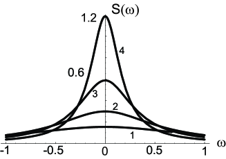
Figure 2: Spectral density of Brownian particle displacement for different values of dimensionless height ($\beta=E/D$) of potential barrier: curve $1$ - $\beta$ $=2$, curve $2$ - $\beta=3$, curve $3$ - $\beta$ $=4$, curve $4$ - $\beta$ $=5$. Parameters are $L=1$, $D=1$.

As shown in Fig. 2, the spectral density has a maximum at zero frequency, which is a general property of Markovian random processes. We see also that the spectrum $S(\omega)$ narrows very rapidly with increasing height of potential barrier, and its value at zero frequency increases fast. This nonlinear phenomenon is due to very rare transitions between steady states when the barrier is high with respect to the noise intensity [17]. Brownian particles therefore move within a potential well for most of the time, and their displacements vary very slowly. As a result, the width of spectral density decreases.

To verify this hypothesis we compare the behaviours of the spectral width and the mean rate of transitions between steady states as a function of potential barrier height. First we find the value of spectral density at zero frequency $S(0)=$ $\tilde{K}\left[0\right]\left/\pi\right.$. Let us expand the function (22) in power series on small parameter $\alpha_{2}$. Then we express this parameter in terms of small parameter $p$

$$\alpha_{2}\simeq-\frac{pL^{2}}{\beta D}+\frac{p^{2}L^{4}}{\beta^{3}D^{2}},$$

and after calculation of the limit $p\rightarrow 0$, we get

$$S(0)=\frac{L^{4}}{\pi D}\cdot\frac{\left(\beta-1\right)^{2}\e^{2\beta}-\left(\beta^{3}-3\beta^{2}+4\beta-4\right)\cdot\e^{\beta}-5}{\beta^{4}\left(\e^{\beta}-1\right)}.$$ (25)

The value $S(0)$ increases therefore as an exponential law $S(0)\sim\e^{\beta}\left/\beta^{2}\right.$, with increasing height of potential barrier $\beta$ and takes the finite value $2L^{4}\left/\left(15\pi D\right)\right.$ for $\beta=0$. This value corresponds to a diffusion in rectangular potential well (see (24)). The width of the spectral density with a maximum at zero frequency can be defined as [16]

$$\Pi=\int\limits_{0}^{+\infty}S(\omega)d\omega\left/S(0)\right.=\frac{\left\langle x^{2}\right\rangle}{2S(0)}.$$ (26)

The variance of Brownian particle position in stationary state from Eqs. (6) and (13) is

$$\left\langle x^{2}\right\rangle=\frac{L^{2}\left[\left(\beta^{2}-2\beta+2\right)\cdot\e^{\beta}-2\right]}{\beta^{2}\left(\e^{\beta}-1\right)}$$ (27)

and increases monotonically from the value $L^{2}\left/3\right.$, which takes for $\beta\rightarrow 0$, to the value $L^{2}$, which takes for $\beta\rightarrow\infty$, due to the finite area of diffusion. Substituting Eqs. (25) and (27) in Eq. (26) we obtain

$$\Pi=\frac{\pi D}{2L^{2}}\cdot\frac{\beta^{2}\left[\left(\beta^{2}-2\beta+2\right)\cdot\e^{\beta}-2\right]}{\left(\beta-1\right)^{2}\e^{2\beta}-\left(\beta^{3}-3\beta^{2}+4\beta-4\right)\cdot\e^{\beta}-5}.$$ (28)

By introducing correlation time similar to (26)

$$\tau_{c}=\int\limits_{0}^{+\infty}K\left[\tau\right]d\tau\left/K\left[0\right]\right.$$

we find from Eqs. (7) and (26)

$$\tau_{c}=\frac{\pi S\left(0\right)}{\left\langle x^{2}\right\rangle}=\frac{\pi}{2\Pi},$$

and equation (28) gives the exact correlation time for bistable potential, recently obtained in [15]. The spectral width decreases monotonically with increasing height of potential barrier from the value $5\pi D\left/\left(4L^{2}\right)\right.$, taken for $\beta\rightarrow 0$, to zero, taken for $\beta\rightarrow\infty$.

The mean rate of transitions, from one stable state to the other, can be determined through the mean first passage time (MFPT) to reach the top of barrier ($x=0$) from the bottom of well ($x=L$), by solving the following differential equation [14, 16] ($x>0$)

$$D\tau^{\prime\prime}\left(x\right)+\frac{E}{L}\tau^{\prime}\left(x\right)=-1$$

with boundary conditions: $\tau^{\prime}\left(L\right)=0$, $\tau\left(0\right)=0$. After simple calculations we get for $\tau(L)$

$$\tau\left(L\right)=\frac{L^{2}}{D}\cdot\frac{\e^{\beta}-1-\beta}{\beta^{2}},$$

and for mean rate of transitions between two steady states

$$\Omega=\frac{D}{L^{2}}\cdot\frac{\beta^{2}}{\e^{\beta}-1-\beta}.$$ (29)

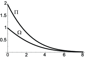
Figure 3: The spectral width and the mean rate of transitions between two steady states vs the dimensionless height of potential barrier. Parameters are $L=1$, $D=0.5$.

In Fig. 3 we report the behaviours of $\Pi$ and $\Omega$ as a functions of dimensionless height of potential barrier $\beta$. The curves expressed by Eqs. (28) and (29) practically coincide at large values of $\beta$. Thus, the mean rate of transitions is approximately the spectral width of Brownian particle coordinate fluctuations in a stationary state.

5 Randomly switching monostable potential

Let us consider now two-noise nonlinear system, namely, one-dimensional overdamped Brownian motion in a fluctuating potential described by the following Langevin equation

$$\frac{dx}{dt}=-\frac{\partial\Phi\left(x,t\right)}{\partial x}+\xi\left(t\right),$$ (30)

where $\xi(t)$ is white Gaussian noise with zero mean and intensity $2D$, $\Phi(x,t)=U(x)+a\eta(t)x$, $U(x)$ is the same potential (13) but without barrier $(E=0)$, and $\eta(t)$ is Markovian dichotomous noise switching with mean rate $\nu$ between the values $\pm 1$. In other words, we analyze Brownian diffusion in monostable potential with two randomly switching stable states near reflecting boundaries at $x=\pm L$ (see Fig. 4).

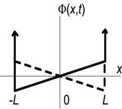
Figure 4: Randomly switching monostable potential.

Let us rewrite for our case the closed set of differential equations for probability density $W(x,t)$, recently obtained in [13], in the diffusion interval $\left(-L,L\right)$

$$\frac{\partial W}{\partial t}=a\frac{\partial Q}{\partial x}+D\frac{\partial^{2}W}{\partial x^{2}},$$

$$\frac{\partial Q}{\partial t}=-2\nu Q+a\frac{\partial W}{\partial x}+D\frac{\partial^{2}Q}{\partial x^{2}}$$ (31)

with the following conditions at reflecting boundaries

$$\left(DW^{\prime}+aQ\right)_{x=\pm L}=0,\qquad\left(DQ^{\prime}+aW\right)_{x=\pm L}=0,$$ (32)

where $Q(x,t)=\left\langle\eta(t)\delta(x-x(t))\right\rangle=W\left(x,t\right)\left\langle\eta(t)\left|x\left(t\right)=x\right.\right\rangle$ is an auxiliary function [13]. We use the same method as for fixed potential.

According to Eqs. (31) and (32) and initial conditions for the functions $W(x,t)$, $Q(x,t)$: $W(x,0)=\delta(x-x_{0})$, $Q(x,0)=0$, we solve the following system of differential equations in the interval $(-L,L)$

$$DY^{\prime\prime}+aZ^{\prime}-pY=-\delta(x-x_{0}),$$

$$DZ^{\prime\prime}+aY^{\prime}-\left(p+2\nu\right)Z=0$$ (33)

with boundary conditions

$$\left(DY^{\prime}+aZ\right)_{x=\pm L}=0,\qquad\left(DZ^{\prime}+aY\right)_{x=\pm L}=0.$$ (34)

Here $Y(x,x_{0},p)$ and $Z(x,x_{0},p)$ are the Laplace transforms of conditional probability density and of auxiliary function respectively. By putting $E=0$ in (16) we get

$$G\left(x_{0},p\right)=\frac{x_{0}}{p}-\frac{D}{p}\left[Y\left(L,x_{0},p\right)-Y\left(-L,x_{0},p\right)\right].$$ (35)

Now we solve the homogeneous set of linear differential equations (33) in two regions: $-L\leq x\leq x_{0}$ and $x_{0}\leq x\leq L$. Then we find eight unknown constants from the boundary conditions (34) and continuity conditions at the point $x=x_{0}$

$$Y\left|{}_{x=x_{0}-0}\right.=Y\left|{}_{x=x_{0}+0}\right.,\qquad Y^{\prime}\left|{}_{x=x_{0}-0}\right.=Y^{\prime}\left|{}_{x=x_{0}+0}\right.+1\left/D\right.,$$

$$Z\left|{}_{x=x_{0}-0}\right.=Z\left|{}_{x=x_{0}+0}\right.,\qquad Z^{\prime}\left|{}_{x=x_{0}-0}\right.=Z^{\prime}\left|{}_{x=x_{0}+0}\right..$$

After some algebra we obtain from (35)

$$G\left(x_{0},p\right)=\frac{x_{0}}{p}$$ (36)

$$-\frac{\left(D\rho_{1}^{2}-p\right)\sinh\rho_{1}L\sinh\rho_{2}x_{0}-\left(D\rho_{2}^{2}-p\right)\sinh\rho_{2}L\sinh\rho_{1}x_{0}}{p\left[\rho_{2}\left(D\rho_{1}^{2}-p\right)\sinh\rho_{1}L\cosh\rho_{2}L-\rho_{1}\left(D\rho_{2}^{2}-p\right)\sinh\rho_{2}L\cosh\rho_{1}L\right]},$$

where

$$\rho_{1,2}=\sqrt{\frac{\gamma^{2}}{2}+\frac{p}{D}\pm\sqrt{\frac{\gamma^{4}}{4}+\frac{pa^{2}}{D^{3}}}},\qquad\gamma=\sqrt{\frac{a^{2}}{D^{2}}+\frac{2\nu}{D}}.$$ (37)

To find the Laplace transform (11) of correlation function in stationary regime we use the expression of SPD for our system, derived in ref. [13],

$$W_{\infty}\left(x\right)=\frac{1}{2L}\cdot\frac{1+\mu\cosh\gamma x\left/\cosh\gamma L\right.}{1+\mu\tanh\gamma L\left/\left(\gamma L\right)\right.},$$ (38)

where $\mu=a^{2}\left/(2\nu D)\right.$. After substitution of Eqs. (36) and (38) into Eq. (11) and integration we get

$$\tilde{K}\left[p\right]=\frac{\left\langle x^{2}\right\rangle}{p}-\frac{1}{p\left[1+\mu\tanh\gamma L\left/\left(\gamma L\right)\right.\right]}$$

$$\times\frac{\left(D\rho_{1}^{2}-p\right)R\left(\rho_{2}\right)\tanh\rho_{1}L-\left(D\rho_{2}^{2}-p\right)R\left(\rho_{1}\right)\tanh\rho_{2}L}{\rho_{2}\left(D\rho_{1}^{2}-p\right)\tanh\rho_{1}L-\rho_{1}\left(D\rho_{2}^{2}-p\right)\tanh\rho_{2}L},$$ (39)

where

$$R\left(z\right)=\frac{1}{z}\left(1-\frac{\tanh zL}{zL}\right)+\frac{\gamma\mu\tanh zL}{z^{2}-\gamma^{2}}\left[\frac{2z}{\left(z^{2}-\gamma^{2}\right)L}-\tanh zL\right]$$

$$+\frac{z\mu}{z^{2}-\gamma^{2}}\left(1-\frac{z^{2}+\gamma^{2}}{z^{2}-\gamma^{2}}\cdot\frac{\tanh zL}{zL}\right).$$ (40)

To obtain the exact formula for the spectral density of Brownian particle position it remains to put in equation (39) $p=i\omega$ and find the real part of expression. In the absence of flippings ($a=0$, $\mu=0$) we find from Eq. (37): $\rho_{1}=\sqrt{\gamma^{2}+p\left/D\right.}$, $\rho_{2}=\sqrt{p\left/D\right.}$ and obtain the result for rectangular potential well of equation (23).

6 New characterization of resonant activation

The evolution of spectrum shape with varying switchings mean rate $\nu$ is shown in Fig. 5. The spectral density of Brownian diffusion in this non-Markovian case has also a maximum at zero frequency.

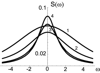
Figure 5: Spectral density $S\left(\omega\right)$ for different values of switchings mean rate $\nu$: curve $1$ - $\nu=0.01$, curve $2$ - $\nu=3$, curve $3$ - $\nu=30$. The curve $4$ corresponds to a free diffusion in rectangular potential well $\left(a=0\right)$. The parameter set is: $L=1$, $a=3$, $D=0.5$.

For very large values of $\nu$, the spectral density approximates to the curve corresponding to a free diffusion in rectangular potential well. The main feature of Fig. 5 is that the spectrum at zero frequency $S\left(0\right)$ shows nonmonotonic behaviour with increasing switchings mean rate $\nu$. Namely, $S\left(0\right)$ initially decreases, reaches a minimum and then increases reaching asymptotically the value $2L^{4}\left/\left(15\pi D\right)\right.$, obtained for rectangular potential well.

Let us find the analytical expression of $S\left(0\right)=\tilde{K}\left[0\right]\left/\pi\right.$. Using the approximate expressions for parameters $\rho_{1}$, $\rho_{2}$ at small $p$ (see (37))

$$\rho_{1}\simeq\gamma+\frac{p}{2\gamma D}\left(1+\frac{a^{2}}{\gamma^{2}D^{2}}\right),\qquad\rho_{2}\simeq\frac{\sqrt{2\nu p}}{\gamma D}$$

and formula for the variance [13]

$$\left\langle x^{2}\right\rangle=\frac{\gamma^{3}L^{3}+3\mu\left[\left(2+\gamma^{2}L^{2}\right)\tanh\gamma L-2\gamma L\right]}{3\gamma^{3}L\left[1+\mu\tanh\gamma L\left/\left(\gamma L\right)\right.\right]}$$ (41)

we get from Eq. (39)

$$S\left(0\right)=\frac{1}{60\pi\gamma^{6}D^{3}\left[1+\mu\tanh\gamma L\left/\left(\gamma L\right)\right.\right]}\{16\nu D\gamma^{4}L^{4}$$

$$+5a^{2}[60+27\mu+4\gamma^{2}L^{2}(3\mu-1)+(4\gamma^{2}L^{2}-27\mu-12)\gamma L\coth\gamma L$$

$$-(48+3\gamma^{2}L^{2}\left(\mu+4\right)-4\gamma^{4}L^{4})\frac{\tanh\gamma L}{\gamma L}]\}.$$ (42)

The typical $\nu$-dependence of spectral density at zero frequency is plotted in Fig. 6. We see a clear minimum at $\nu\simeq 3$. To explain this minimum let us consider the resonant activation phenomenon for this system.

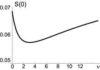
Figure 6: Nonmonotonic behaviour of the spectral density at zero frequency as a function of mean rate of flippings, for the same parameters $L$, $a$, $D$ of Fig. 5.

From the closed set of differential equations for MFPTs $T_{+}\left(x\right)$ and $T_{-}\left(x\right)$ [18]

$$DT_{+}^{\prime\prime}-aT_{+}^{\prime}+\nu\left(T_{-}-T_{+}\right)=-1,$$

$$DT_{-}^{\prime\prime}-aT_{-}^{\prime}+\nu\left(T_{+}-T_{-}\right)=-1$$ (43)

we calculate $T_{+}\left(x\right)$ and $T_{-}\left(x\right)$, the MFPTs for positive $\eta\left(0\right)=+1$ and negative $\eta\left(0\right)=-1$ initial value of the dichotomous noise, with starting position of Brownian particles at the point $x$, respectively. If we place the absorbing boundary at the point $x=L$ we solve equations (43) with the following boundary conditions: $T_{\pm}^{\prime}\left(-L\right)=0,\;T_{\pm}\left(L\right)=0.$ The arithmetic average of MFPTs $T\left(x\right)=\left[T_{+}\left(x\right)+T_{-}\left(x\right)\right]\left/2\right.$ for initial position of Brownian particles at the point $x=-L$ is

$$T\left(-L\right)=\frac{4\nu L^{2}}{\gamma^{2}D^{2}}+\frac{a^{2}}{\gamma^{4}D^{3}}\left[\cosh 2\gamma L-1-\frac{\left(\sinh 2\gamma L-2\gamma L\right)^{2}}{\cosh 2\gamma L+\mu}\right].$$ (44)

The behaviour of $T(-L)$ as a function of switchings mean rate has a minimum, as shown in Fig. 7.

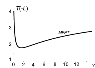
Figure 7: Resonant activation phenomenon for MFPT $T\left(-L\right)$. The parameters $L$, $a$ and $D$ are the same as in Fig. 6.

This effect was called in literature resonant activation: the average residence time as a function of the barrier fluctuation rate $\nu$ has a minimum at intermediate rates between very slow and very fast fluctuations [2]. In this range of rate $\nu$, the crossing event is strongly correlated with the potential fluctuations and Brownian particles overcome randomly switching barrier in a minimal time. As a result, Brownian particle position changes rapidly and very slow components of the random process $x\left(t\right)$ are present in minor amounts: the spectral density at zero frequency takes a minimum. Thus, the nonmonotonic behaviour of the spectral density at zero frequency $S\left(0\right)$ can be interpreted as a new characterization of resonant activation phenomenon.

Finally we report in Fig. 8 the behaviour of spectral width $\Pi$ as a function of flippings mean rate $\nu$.

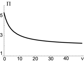
Figure 8: Spectral width vs flippings mean rate for the same parameters $L$, $a$ and $D$ of Fig. 5.

We find a new nonlinear phenomenon: the spectral width decreases with increasing mean rate of switchings, contrary to the linear behaviour. As switchings mean rate increases, the slope of the potential profile of Fig. 4 becomes less and less important. As a result, the diffusion time of Brownian particle between the reflecting boundaries $x=\pm L$ increases and is determined by a free diffusion at very fast flippings. The random process $x\left(t\right)$ therefore becomes more slow and the spectral width $\Pi$ decreases.

7 Conclusions

The exact formula for the spectral density of diffusion in double-well potential for arbitrary noise intensity and arbitrary parameters of potential profile was obtained. We found very rapid narrowing of the spectrum with increasing height of a potential barrier between steady states. We also derived the exact result for spectral density of fluctuations in two-noise nonlinear system, namely, for overdamped Brownian diffusion in randomly flipping potential. We found a new characterization of resonant activation phenomenon in the behaviour of spectral density at zero frequency and new nonlinear effect associated with narrowing of the spectrum of Brownian particle position with increasing mean rate of switchings. Our analytical method enable us to investigate more difficult problems as those with more complex potential profiles. 

This work has been supported by INTAS Grant 2001-0450, MIUR, INFM, by Russian Foundation for Basic Research (project 02-02-17517), by Federal Program ”Scientific Schools of Russia” (project 1729.2003.2), and by Scientific Program ”Universities of Russia” (project 01.01.020).

References

- [1] L. Gammaitoni, P. Hänggi, P. Jung, F. Marchesoni, Rev. Mod. Phys. 70, 223 (1998); R.N. Mantegna, B. Spagnolo, Phys. Rev. E49, R1792 (1994); R.N. Mantegna, B. Spagnolo, M. Trapanese, Phys. Rev. E63, 011101 (2001); E. Lanzara, R.N. Mantegna, B. Spagnolo, R. Zangara, Am. J. Phys. 65, 341 (1997).
- [2] C.R. Doering, J.C. Gadoua, Phys. Rev. Lett. 69, 2318 (1992); M. Bier, R.D. Astumian, Phys. Rev. Lett. 71, 1649 (1993); U. Zürcher, C.R. Doering, Phys. Rev. E47, 3862 (1993); R.N. Mantegna, B. Spagnolo, J. Phys. IV France 8, 247 (1998); R.N. Mantegna, B. Spagnolo, Phys. Rev. Lett. 84, 3025 (2000).
- [3] R.N. Mantegna, B. Spagnolo, Phys. Rev. Lett. 76, 563 (1996); N.V. Agudov, A.N. Malakhov, Phys. Rev. E60, 6333 (1999); N.V. Agudov, B. Spagnolo, Phys. Rev. E64, 035102(R) (2001); A. Fiasconaro, D. Valenti, B. Spagnolo, Physica A325, 136 (2003); A. Fiasconaro, D. Valenti, B. Spagnolo, Modern Problems of Statistical Physics 2, 101 (2003).
- [4] N.V. Agudov, A.A. Dubkov, B. Spagnolo, Physica A325, 144 (2003).
- [5] M.O. Magnasco, Phys. Rev. Lett. 71, 1477 (1993); F. Jülicher, A. Ajdari, J. Prost, Rev. Mod. Phys. 69, 1269 (1997).
- [6] P. Reimann, Phys. Rep. 361, 57 (2002).
- [7] T.K. Caughey, J.K. Dienes, J. Appl. Phys. 32, 2476 (1961).
- [8] M. Mörsch, H. Risken, H.D. Vollmer, Z. Physik B32, 245 (1979).
- [9] M.I. Dykman, R. Mannella, P.V.E. McClintock, F. Moss, S.M. Soskin, Phys. Rev. A37, 1303 (1988); M.I. Dykman, R. Mannella, P.V.E. McClintock , S.M. Soskin, N.G. Stocks, Phys. Rev. A42, 7041 (1990); M.I. Dykman, R. Mannella, P.V.E. McClintock , S.M. Soskin, N.G. Stocks, Phys. Rev. A43, 1701 (1991); M.I. Dykman, P.V.E. McClintock, Physica D58, 10 (1992); M.I. Dykman, K. Lindenberg, in Contemporary Problems in Statistical Physics, edited by G.H. Weiss, SIAM, Philadelphia 1994, p.41.
- [10] F. Marchesoni et al., Phys. Rev. A37, 3058 (1988).
- [11] H.F. Ouyang, Z.Q. Huang, E.J. Ding, Phys. Rev. E50, 2491 (1994).
- [12] N.V. Agudov, A.A. Dubkov, B. Spagnolo, in “Noise in Physical Systems and 1/f Fluctuations”, ed. by G. Bosman, Gainesville, Florida, USA (2001), p.612.
- [13] A.A. Dubkov, P.N. Makhov, B. Spagnolo, Physica A325, 26 (2003).
- [14] H. Risken, The Fokker-Planck Equation, Springer, Berlin 1984; M. v. Smoluchowski, Ann. Physik 48, 1103 (1915).
- [15] A.A. Dubkov, A.N. Malakhov, A.I. Saichev, Radiophys. and Quantum Electronics 43, 335 (2000).
- [16] R.L. Stratonovich, Topics in the Theory of Random Noise, Gordon and Breach, New York 1963, Vol.1.
- [17] H.A. Kramers, Physica 7, 284 (1940).
- [18] V. Balakrishnan, C. Van den Broeck, P. Hänggi, Phys. Rev. A38, 4213 (1988).