Quantum Creep and Variable Range Hopping of One-dimensional Interacting Electrons

Abstract

The variable range hopping results for noninteracting electrons of Mott and Shklovskii are generalized to 1D disordered charge density waves and Luttinger liquids using an instanton approach. Following a recent paper by Nattermann, Giamarchi and Le Doussal [Phys. Rev. Lett. 91, 56603 (2003)] we calculate the quantum creep of charges at zero temperature and the linear conductivity at finite temperatures for these systems. The hopping conductivity for the short range interacting electrons acquires the same form as for noninteracting particles if the one-particle density of states is replaced by the compressibility. In the present paper we extend the calculation to dissipative systems and give a discussion of the physics after the particles materialize behind the tunneling barrier. It turns out that dissipation is crucial for tunneling to happen. Contrary to pure systems the new metastable state does not propagate through the system but is restricted to a region of the size of the tunneling region. This corresponds to the hopping of an integer number of charges over a finite distance. A global current results only if tunneling events fill the whole sample. We argue that rare events of extra low tunneling probability are not relevant for realistic systems of finite length. Finally we show that an additional Coulomb interaction only leads to small logarithmic corrections.

I Introduction

In one dimensional systems, the interplay of interaction and disorder gives rise to a variety of interesting physical phenomena Giamarchi ; Gruner ; Giamarchi+Schulz ; KaneFisher ; FuNa93 ; YuGlMa94 ; ll78 ; Finkelstein83 . In and below two dimensions, disorder leads to localization of all electronic states mt61 ; BeKi94 ; Berezinskii73 ; Abrahams+79 ; OpWe79 ; VoWo80 . Interactions lead to a breakdown of the Fermi liquid concept in one dimension and to the emergence of a Luttinger liquid instead Haldane ; KaneFisher ; Giamarchi , which is characterized by collective excitations. In 1d electron systems, these strong perturbations compete with each other. In the presence of a repulsive interaction, disorder is a relevant perturbation and drives the system into a localized phase Giamarchi+Schulz ; BeKi94 . As a result the linear conductivity vanishes at zero temperature. Thermal fluctuations destroy the localized phase Glatz+Natter02 ; Glatz+Natter04 . At sufficiently high temperatures, i.e. if the thermal de Broglie wavelength of the collective excitations becomes shorter than the zero temperature localization length, the linear conductivity exhibits a power law dependence on temperature with interaction dependent exponents Giamarchi+Schulz . At very low temperatures noninteracting electrons show hopping conductivity Mott69 ; ahl71 ; Shklovskii_Efros_Book . In the present paper we study both, the nonlinear conductivity due to strong electric fields in the zero temperature localized phase as well as the finite temperature hopping conductivity for interacting systems.

Interaction effects in 1d electron systems can be described by the method of bosonization Haldane , which directly describes the collective degrees of freedom associated with the oscillations of a string. Due to the quantum nature of the system, the string can be viewed as a two dimensional elastic manifold in a three dimensional embedding space. In the localized phase, this manifold is pinned by the impurity potential. For a classical pinned manifold, thermally activated hopping over barriers leads to thermal creep, i.e. a nonlinear current-voltage characteristic IoVi87 ; Na87 . Due to the quantum nature of the bosonized electron system, thermal hopping is replaced by quantum tunneling giving rise to quantum creep ngd03 .

From a quantum mechanical point of view, tunneling driven by a potential gradient corresponds to the decay of a metastable state. Using a field theoretical language, this decay is described by instantons langer ; Schulman ; tHooft ; Coleman , i.e. solutions of the Euclidean saddle point equations with a finite action. In the presence of a periodic potential, instantons relate ground states which differ by a multiple of $2\pi$. In this way, the nucleation of a new ground state takes place. The instanton picture was used by Maki Maki to study the nonlinear conductivity of the quantum sine Gordon model. Recently, this framework was used to describe quantum creep in a sine Gordon model with random phase shifts ngd03 , which models the physics of disordered and short range interacting 1d electrons in the localized phase.

In the quantum sine Gordon model, instanton formation is followed by materialization of a kink particle. The materialization is characterized by a rapid expansion of the instanton in both space and time. During this expansion process of the new ground state, the kink particle moves according to its equation of motionMaki . Within the Euclidean action approach, the instanton expansion is described by an unstable Gaussian integral over the saddle point, which gives rise to an imaginary part of the partition function describing the instability of the metastable state langer . In the disordered case, instanton formation describes tunneling from an occupied site close to the Fermi surface to a free site close to it. However, spatial motion of the kink particle after its materialization is impeded by new barriers.

The central point of our paper is a discussion of the materialization process in the disordered case: an extension of the instanton is only possible in time direction due to the presence of barriers in space direction. The inclusion of dissipation feynman ; CaldeiraLeggett ; Hida+Eckern ; Kleinert ; Weiss99 is essential for this process to occur. A dissipative term in the action is essential for finding a saddle point associated with an unstable Gaussian integral on the one hand. On the other hand, dissipation is necessary to correct the energy balance. It is this aspect which was missing in the earlier publication ngd03 . The external electric field provides for the energy necessary to tunnel from an occupied site below the Fermi level to an unoccupied site slightly above it. Generally, the gain in field energy will be larger than the energy difference of the two levels. As dissipation corresponds to the possibility of inelastic processes, the excess energy can be absorbed by the dissipative bath. In the absence of an additional bath, the conductivity was suggested to decay in a double exponential manner with decreasing temperature GMP04 .

The discussion of the instanton mechanism is combined with an RG analysis of the disordered system Glatz+Natter02 ; Glatz+Natter04 . As a consequence, only effective parameters obtained from RG enter the results. The combination with an RG is necessary to scale the system into a regime where the quasiclassical instanton analysis is applicable.

We make a detailed comparison to Mott Mott69 ; ahl71 variable range hopping of noninteracting particles and generalize an argument due to Shklovskii s73 for tunneling of localized electrons in strong fields to arbitrary dimensions. The instanton mechanism discussed above describes the same type of physics. We also discuss the influence of long range interaction Efros_Shklovskii .

We compare the physics of quantum creep to a field induced delocalization transition discovered by Prigodin Prigodin80 ; Soukoulis+83 ; DeSiSo84 ; Kirkpatrick86 ; PriAl89 . This transition is due to the energy dependence of the backscattering probability from a single impurity. As the energy depends linearly on position in the presence of an external electric field, the localization length acquires a spatial dependence. If the localization length grows sufficiently fast, the wave function is no longer normalizable and the state is delocalized. We show that this mechanism becomes effective at field strengths which are parametrically larger than the crossover field for which quantum creep becomes important. In addition, we discuss a generalization of this mechanism to interacting systems. We find that for repulsive short range interactions the delocalizing effect of an external field is less pronounced (in our approximation it even completely disappears) and hence delocalization is not a relevant competition for quantum creep. For attractive short range interactions, the delocalizing effect of an external field is enhanced.

The organization of the paper is as follows: in section II we set up the model and discuss its renormalization. The tunneling due to instantons and the subsequent time evolution of the quantum sine Gordon system is discussed as a reference point in section III. Based on this analysis, tunneling in the disordered case and the essential influence of dissipation is presented in section IV. In section V we compare with previous results for noninteracting systems obtained by Shklovskii and Mott, in section VI we study the influence of a long range Coulomb interaction, and in section VII we discuss the relevance of a localization-delocalization transition in external fields to the problem of quantum creep in 1d systems.

II Model and zero-field renormalization

II.1 The model

We consider in this paper disordered charge- or spin density waves or Luttinger liquids with a density Gruner ; Haldane ; Giamarchi

$$\rho=\left(\rho_{0}+\frac{1}{\pi}\partial_{x}\varphi\right)\big{(}1+\Delta\cos(p\varphi+Qx)\big{)}\,.$$ (2.1)

Here $p=1,2$ for charge density waves (CDW) and Luttinger liquids (LL), respectively, and $p\rho_{0}=(1/\pi)Q$. The form (2.1) preserves the conservation of the total charge under an arbitrary deformation $\varphi(x)$, provided $|\nabla\varphi|\ll Q$. The wave vector of the density modulation $Q=2k_{F}$ for LLs and CDWs (although the value of $Q$ can be different for CDWs depending on the precise shape of the 3D Fermi surface and the optimal electron phonon coupling), and $Q=4k_{F}$ for spin density waves (SDWs). $\Delta=2$ for LLs with a strictly linear dispersion relationHaldane whereas for CDWs $\sqrt{\rho_{0}\Delta}$ denotes the amplitude of the order parameter of the condensate.

The Hamiltonian of the corresponding disordered system is then given by

$$\hat{\mathcal{H}} = \frac{1}{2\pi}\int dx\bigg{\{}\hbar vK(\pi\hat{\Pi})^{2}+\frac{\hbar v}{K}(\partial_{x}\hat{\varphi})^{2}$$ (2.2)

$$+2\pi\rho(x)\big{(}-Exe_{0}+U_{R}(x)\big{)}\bigg{\}}\,,$$

where $\hat{\Pi}(x)$ denotes the momentum operator conjugate to $-\hat{\varphi}(x)$:

$$\big{[}\hat{\Pi}(x),\hat{\varphi}(x^{\prime})\big{]}=i\delta(x-x^{\prime})\,,$$ (2.3)

$v$ denotes the velocity of the phason excitations, and $K$ is the measure of short range interactions. The quantities can be expressed as $\frac{v}{K}=\frac{1}{\pi\hbar\kappa}$, $vK=\frac{\pi\hbar\rho_{0}}{m}$ and hence $K^{2}=\frac{\pi^{2}\hbar^{2}\rho_{0}\kappa}{m}$ and $v^{2}=\frac{\rho_{0}}{m\kappa}$ where $\kappa$ is the compressibility and $m$ the effective mass of the charge carriers (for more details see Appendix A).

For noninteracting spinless fermions $K=1$ and $v=v_{F}$ where $v_{F}$ denotes the Fermi velocity. In CDWs $K$ is small, of the order $10^{-2}$ whereas in SDWs $K$ may reach one Gruner . $E$ denotes the external electric field.

The random potential $U_{R}(x)$ is considered to be build of isolated impurities at random positions $x_{i}$, $i=1,\ldots,N_{\text{imp}}$:

$$U_{R}(x)=-u_{0}\sum\limits_{i=1}^{N_{\text{imp}}}\delta(x-x_{i})\,.$$ (2.4)

In the following, we will neglect the forward scattering term $\sim\partial_{x}\varphi U_{R}(x)$ since it does not affect the time dependent properties. Since disorder is assumed to be weak and hence effective only on length scales much larger than the impurity spacing, we may rewrite the backward scattering term in the continuum manner:

$$-\rho_{0}\Delta u_{0}\int dx\sum\limits_{i=1}^{N_{\text{imp}}}\delta(x-x_{i})\cos(p\varphi(x)+Qx)$$ (2.5)

$$\to-\rho_{0}\Delta u_{0}n^{1/2}_{\text{imp}}a^{-1/2}\int dx\cos\big{(}p\varphi+\alpha(x)\big{)}\,.$$

Here $n_{\text{imp}}=N_{\text{imp}}/L$ is the impurity concentration, and $\alpha(x)$ is a random phase equally distributed in the interval $0\leq\alpha<2\pi$ and $\overline{e^{i(\alpha(x)-\alpha(y))}}=a\delta(x-y)$. For weak pinning, the replacement (2.5) is valid on length scales much larger than the mean impurity spacing and can be justified by the fact that both parts of (2.5) lead to the same pair correlations , e.g. the same replica Hamiltonian

$$-\frac{1}{2}(\rho_{0}\Delta u_{0})^{2}n_{imp}\int dx\cos\left(p(\varphi_{\alpha}(x)-\varphi_{\beta}(x)\right).$$ (2.6)

and hence to the same physics.

The effective Hamiltonian can therefore be rewritten as

$$\begin{split}\hat{\mathcal{H}}&=\frac{1}{2\pi}\int dx\bigg{\{}\hbar vK(\pi\hat{\Pi})^{2}+\frac{\hbar v}{K}(\partial_{x}\varphi)^{2}\\ &-2e_{0}\hat{\varphi}E-2\pi\rho_{0}\Delta n^{1/2}_{\text{imp}}a^{-1/2}u_{0}\cos\big{(}p\varphi+\alpha(x)\big{)}\bigg{\}}\,.\end{split}$$ (2.7)

Below we will use an imaginary time path integral formulation. It is convenient to use dimensionless space and time coordinates by changing $x/a\to x$ and $v\tau/a\to y$ where $a$ is a small scale cut-off. The Euclidean action of our system is then given by

$$\frac{S}{\hbar} = \frac{1}{2\pi K}\int dx\int\limits_{-K/2T}^{K/2T}dy\Big{\{}(\partial_{y}\varphi)^{2}+(\partial_{x}\varphi)^{2}$$ (2.8)

$$-2f\varphi-2u\cos\big{(}p\varphi+\alpha(x)\big{)}\Big{\}}\,.$$

The dimensionless parameters of the theory are

$$\begin{split}K,\,\,\,\,\,\,\,T=\frac{Ka}{\hbar\beta v},\,\,\,\,\,\,\,f=e_{0}Ea\beta T=\frac{Ke_{0}Ea^{2}}{\hbar v},\\ u=\frac{2\pi a^{3/2}K\rho_{0}\Delta n^{1/2}_{\text{imp}}u_{0}}{\hbar v}.\end{split}$$ (2.9)

$\beta$ is the inverse temperature. All $p$-dependent physical quantities $Q(p;K,T,u,f)$ can be calculated from the case $p=1$ by the relation

$$Q(p;K,T,u,f)=Q(1;p^{2}K,p^{2}T,p^{2}u,pf).$$ (2.10)

II.2 Renormalization group analysis

Our strategy to consider the transport properties of the present one-dimensional system includes two steps.

(i) We first integrate out phase fluctuations on length scales from the initial microscopic cut-off $a=1$ to $\xi=e^{l^{*}}$ $1<e^{l}<\xi$ keeping $f=0$; $\xi$ is determined from the condition that the renormalized and rescaled coefficient $u(l)$ of the nonlinear term in (2.8) becomes of order of one or larger and, typically, $K$ becomes small.

(ii) In the second step we treat the problem at nonzero $f$ in the quasi-classical limit. Corrections to this quasi-classical limit arise if the renormalized $K$ is still of order one.

Since the first step is well documented in the literature we will here quote only the results. At zero temperature and $f=0$ the flow equations are given by Giamarchi+Schulz ; Glatz+Natter04

$$\begin{split}\frac{dK}{dl}&=-\frac{1}{2}p^{4}u^{2}KB_{0}(p^{2}K)\,,\\ B_{0}(x)&=\int\limits_{0}^{\infty}d\tau\,\tau^{2}e^{-\tau}\left(1+\frac{\tau^{2}}{2}\right)^{-x/4}\,.\end{split}$$ (2.11)

$$\frac{du^{2}}{dl}=\left(3-\frac{p^{2}}{2}K\right)u^{2}\,.$$ (2.12)

For completeness we also quote the flow equation in the case when the phase $\alpha(x)$ is fixed at $\alpha=0$:

$$\frac{dK}{dl} = -\frac{1}{8\pi}p^{4}u^{2}B_{2}(p^{2}K)\,,$$ (2.13)

$$B_{2}(x) = \int\limits_{0}^{\infty}d\tau\,dx\,(x^{2}+\tau^{2})e^{-\tau}\left(1+\frac{\tau^{2}}{2}\right)^{-x/4}\!\!\cos x\,,$$

$$\frac{du}{dl} = \left(2-\frac{p^{2}}{4}K\right)u\,.$$ (2.14)

Note that in this pure case the definition of $u$ in (2.9) contains an additional factor $\sqrt{n_{\text{imp}}a}$.

In both cases (2.11, 2.12) and (2.13, 2.14), there is a phase transition at $K=K_{c}(u)$ with $K_{c}(0)=6/p^{2}$ and $K_{c}(0)=8/p^{2}$, respectively. For $K>K_{c}$ the potential becomes irrelevant and the system is in a superconducting phase. For $K<K_{c}$ the asymptotic $RG$-flow is to small values of $K$ and large values of $u$. For the rest of the paper we will restrict ourselves to the case $K<K_{c}$.

The renormalization was done so far for zero external field. Now we switch on the field which is a relevant perturbation and destabilizes the system. As in the previous section we consider on scales $L<\xi$ only fluctuations inside one potential valley. The field is then rescaled according to

$$\frac{df}{dl}=2f(l)\,.$$ (2.15)

According to our strategy we stop the flow at $l=l^{\ast}$, $e^{l^{\ast}}=\xi$, $p^{2}u(l^{\ast})=\mathcal{M}$ with $\mathcal{M}\geq 1$ (see Fig. 1). Clearly our one loop flow equations break down as soon as $u(l)\sim 1$, but qualitatively we expect that the flow continues to go into the direction of large $u$ and simultaneously small $K$ such that typically $K(l^{\ast})\ll 1$. The restricted validity of the one-loop flow equations will then merely result in the uncertainty of the definition of the value $K(l^{\ast}(\cal{M}))$.

Figure 1: Flow diagram in $K-u$ plane. RG is stopped at scale $l=l^{\ast}$ such that $p^{2}u(l^{\ast})=\mathcal{M}\gg 1$.

The quantities $u(l)$ and $K(l)$ are the renormalized and rescaled parameters. The corresponding effective parameters observed on scale $L=e^{l}$ are unrescaled. In pure systems $K_{\rm eff}(L)=K(l)$, $u_{\rm eff}(L)=e^{-2l}u(l)$, and $f_{\rm eff}(L)=f=e^{-2l}f(l)$. In this way we get $u_{\rm eff}(\xi)\approx\mathcal{M}/(p\xi)^{2}$.

For impure systems the corresponding relations are $K_{\rm eff}(L)=K(l)$, $u^{2}_{\rm eff}(L)=e^{-3l}u^{2}(l)$, $f_{\rm eff}(L)=f=e^{-2l}f(l)$ and we get $u^{2}_{\rm eff}(\xi)\approx\mathcal{M}/(p^{2}\xi^{3})$. Not too close to $K_{c}$, $\xi$ can be written as

$$\xi\sim L_{\rm FL}^{\frac{K_{c}}{K_{c}-K}}$$ (2.16)

where $L_{\rm FL}=a(p^{2}u)^{-2/3}$ denotes the Fukuyama-Lee length. $\xi$ has the physical meaning of a correlation length. Note, that in the disordered case there is no renormalization of

$$\frac{v}{K}=\frac{v_{\mathrm{eff}}}{K_{\mathrm{eff}}}=\frac{1}{\pi\hbar\kappa}$$ (2.17)

because of a statistical tilt symmetry USchultz .

III Tunneling - in the pure case

At low but finite temperature the lifetime $\Gamma^{-1}$ of a metastable state is determined by quantum-mechanical tunneling and given by the relation

$$\hbar\Gamma=-2\operatorname{Im}F=2\beta^{-1}\operatorname{Im}\ln Z\,,$$ (3.1)

where $F$ is the free energy. In the path integral formulation $Z$ is given by

$$Z=Z_{0}+iZ_{1}=\int{\mathcal{D}}\varphi(x,\tau)\,e^{-\frac{1}{\hbar}\int\limits_{-K_{\mathrm{eff}}/2T}^{K_{\mathrm{eff}}/2T}dy\,{\mathcal{L}}\big{(}\{\varphi\},f\big{)}}.$$ (3.2)

Here ${\mathcal{L}}\big{(}\{\varphi\},f\big{)}$ denotes the Lagrangian of the metastable system from which we integrated out already fluctuations on length scales smaller than $\xi$. This resulted in the replacement $u\to u_{\mathrm{eff}}(l^{\ast})$ and $K\to K_{\mathrm{eff}}(l^{\ast})$. $f$ represents the driving force. The contribution $Z_{0}$ of the partition function $Z$ contains the contribution from field configurations restricted to stay in the vicinity of the potential minimum. Configurations which leave the metastable state are unstable and contribute to the imaginary part of the free energy, which is assumed to be small such that

$$\Gamma\approx 2(\beta\hbar)^{-1}\frac{Z_{1}}{Z_{0}}\,.$$ (3.3)

What we will do in the following is the calculation of the tunneling probability in the quasi-classical approximation: assuming that $K_{\text{eff}}=K(l^{\ast})\ll 1$ we assume that the only deviation from a completely classical behavior is the generation of instantons which trigger the decay of the metastable state. Before we come to the disordered case we briefly exemplify the physics on the pure sine-Gordon model which facilitates the further discussion. The imaginary time Lagrangian of the sine-Gordon model is given by

$$-{\mathcal{L}}\big{(}\{\varphi\}\big{)} = \int\limits_{0}^{L_{0}/a}dx\frac{1}{2\pi K_{\mathrm{eff}}}\bigg{\{}\left(\frac{\partial\varphi}{\partial y}\right)^{2}+\left(\frac{\partial\varphi}{\partial x}\right)^{2}$$ (3.4)

$$-2u_{\mathrm{eff}}\cos p\varphi-2f\varphi\bigg{\}}\,.$$

The decay of a metastable state (say $\varphi_{0}=0$) of the sine-Gordon model has been first considered by Maki Maki following earlier considerations by t’Hooft tHooft and Coleman Coleman . In the present framework the tunneling process is represented by the formation of a two-dimensional instanton which obeys the Euclidean field equation

$$\frac{\partial^{2}}{\partial y^{2}}\varphi+\frac{\partial^{2}}{\partial x^{2}}\varphi-pu_{\mathrm{eff}}\sin p\varphi+f=0$$ (3.5)

and has a finite Euclidean action. The instanton solution $\varphi_{s}(x,y)$ we are looking for forms a (spherical) droplet in the new metastable minimum $\varphi_{1}=2\pi$. Using spherical coordinates, $r^{2}=x^{2}+y^{2}$, we get from (3.5)

$$\frac{\partial^{2}}{\partial r^{2}}\varphi+\frac{1}{r}\frac{\partial}{\partial r}\varphi-pu_{\mathrm{eff}}\sin p\varphi+f=0\,.$$ (3.6)

For small $f$ and hence large droplet radii $R$ we may drop the second term. In particular for $f=0$ the solution is

$$\varphi(r)=\frac{4}{p}\arctan\exp\big{[}(R-r)\sqrt{\pi u_{\mathrm{eff}}p^{2}}\big{]}$$ (3.7)

which connects the original state $\varphi(r)=0$ for $r-R\gg w$ with the new (likewise metastable) state $\varphi(r)=2\pi/p$ for $R-r\gg w$ where $w=1/\sqrt{p^{2}u_{\mathrm{eff}}}\approx\xi\big{/}\sqrt{\cal M}$ is the width of the droplet wall. The neglect of the second term in (3.6) is justified for $R\gg w$. In the following, we will use this narrow wall approximation to describe the instanton only by its radius ignoring for the moment the shape fluctuations. The action of the instanton includes then a surface and a bulk contribution

$$\frac{S(R)}{\hbar}=\frac{2\pi}{pK_{\mathrm{eff}}}\left(R\sigma-R^{2}f\right)\ ,$$ (3.8)

where $\sigma=\frac{8\sqrt{u_{\mathrm{eff}}}}{\pi}\approx\frac{8}{\pi}\frac{\sqrt{\cal M}}{p\xi}$ is the surface tension of the instanton (the Euclidean action associated with the unit length of the instanton boundary is equal to $\hbar\sigma/(pK)$). The action (3.8) has a maximum at

$$R_{c}=\sigma\big{/}(2f).$$ (3.9)

where ${S(R_{c})}/{\hbar}\equiv{S_{\text{inst}}}/{\hbar}={\pi\sigma^{2}}/({2pK_{\mathrm{eff}}f})$ denotes the instanton action.

The ratio $iZ_{1}/Z_{0}$ appearing in the (3.3) can now be calculated as a functional integral over circular droplets Kleinert

$$\begin{split}\frac{Z_{1}}{Z_{0}}\propto{\rm Im\,}\int\sqrt{\frac{S_{\text{inst}}}{{\hbar}}}dR\,e^{-S(R)/\hbar}\\ \propto e^{-S_{\text{inst}}/{\hbar}}{\rm Im\,}\int\limits_{-R_{c}}^{\infty}dr\sqrt{\frac{S_{\text{inst}}}{{\hbar}}}\,e^{2\pi fr^{2}/(pK_{\mathrm{eff}})}\,.\end{split}$$

Here we have taken into account that the change from the integration over $\varphi$ to $R$ involves a Jacobian $\sim\sqrt{S_{\text{inst}}/\hbar}$. The integral, taken along the real axis, is divergent since the saddle point (in the functional space) is a maximum of the action as a function of the instanton size $R=R_{c}+r$.

This leads – after the proper analytic continuation – to the imaginary part in $iZ_{1}$ in the partition function (for a more detailed discussion see Schulman Schulman ). As a result we obtain

$$\frac{iZ_{1}}{Z_{0}}\propto{i}\frac{R_{c}}{\xi}e^{-{S_{\text{inst}}}/{{\hbar}}}\,.$$ (3.10)

Further contributions to the pre-exponential term result from the inclusion of fluctuations of the shape of the instanton. Within the narrow wall approximation these fluctuations could be taken into account by rewriting the Euclidean action in the form DiehlKrollWagner

$$\frac{S}{\hbar}=\frac{1}{pK_{\mathrm{eff}}}\sum\limits_{k=\pm}\!\int\limits_{-K_{\mathrm{eff}}/2T}^{K_{\mathrm{eff}}/2T}\!\!\!\!dy\left\{\sigma\sqrt{1+(\partial_{y}X_{k})^{2}}-2kfX_{k}(y)\right\}.$$ (3.11)

$X_{k}(y)$ (where $k=\pm$) denote the wall position of the left and right segment of the wall of the critical droplet, respectively. These fluctuations were considered by Maki Maki , they lead to a downward renormalization of the surface tension in (3.11).

So far we considered the center of the instanton to be fixed at $x=X_{0}$ and $y=0$. However the position of the center can be moved around which corresponds to the existence of two modes with zero eigenvalue. Correspondingly, in the calculation of the partition function we have to integrate over all possible instanton positions which delivers in the low temperature limit

$$\frac{K_{\text{eff}}}{T}\gg R_{c}=\frac{\sigma}{2f}$$ (3.12)

an additional factor Coleman

$$\frac{L_{0}K_{\text{eff}}}{T\xi^{2}}\frac{S_{\text{inst}}}{2\pi\hbar}\,,$$ (3.13)

where $L_{0}$ is the sample length. The first factor counts the number of different instanton positions, the second one is the Jacobian resulting from the transition from the original to the displacement degrees of freedom. Thus

$$\Gamma\sim\frac{L_{0}\sigma^{3}}{p\beta Tf^{2}\xi^{3}}e^{-\pi\sigma^{2}/(2pK_{\text{eff}}f)}\,.$$ (3.14)

$\Gamma^{-1}$ represents the time scale on which the phase field $\varphi$ tunnels through the energy barrier between $\varphi_{0}$ and $\varphi_{1}$.

Once the critical droplet of the new ground state $\varphi_{1}$ is formed, the field materializes and evolves subsequently according to the classical equation of motion Coleman .

The latter follows from Eq. (3.5) by the resubstitution $y=ivt$. Since $\varphi_{s}(r)$ depends only on $r^{2}=x^{2}-v^{2}t^{2}$, the solution of Eq. (3.6) also describes the evolution of the phase field after the tunneling event. Within the narrow wall approximation, the Minkowski action is

$$\frac{S_{M}}{\hbar}=-\frac{\sigma}{pK_{\mathrm{eff}}}\sum\limits_{k=\pm}\int dt\,\bigg{\{}\sqrt{1-\frac{\dot{X}_{k}^{2}(t)}{v^{2}}}-k\frac{X_{k}(t)}{R_{c}}\bigg{\}}\ ,$$ (3.15)

which leads to the equation of motion of two relativistic particles

$$\pm\frac{1}{v^{2}}\frac{d}{dt}\frac{\dot{X}_{\pm}(t)}{\sqrt{1-\dot{X}_{\pm}^{2}/v^{2}}}=R_{c}^{-1}\,.$$ (3.16)

This has to be solved with the initial condition $X_{\pm}(t=0)=X_{0}\pm R_{c}$ where $t=0$ corresponds to the moment of the materialization, hence

$$X_{\pm}(t)=\pm\sqrt{R_{c}^{2}+v_{\text{eff}}^{2}t^{2}}+X_{0}\,.$$ (3.17)

Clearly, with $ivt\to y$, this is also the saddle-point equation of action (3.11), corresponding again to a spherical droplet of radius $R_{c}$.

The energy ${\cal E}$ is a conserved quantity during the motion of the kinks as

$${\cal E}=\frac{\hbar\sigma}{p}\sum_{k=\pm}\Big{\{}\frac{1}{\sqrt{1-\dot{X}_{k}^{2}/v^{2}}}-k\frac{X_{k}}{R_{c}}\Big{\}}=0.$$ (3.18)

Since the potential energy of the new metastable state is always lower than that of the initial configuration the kinks will accelerate, approaching eventually the phason velocity $v_{\text{eff}}$.

In a long sample the nucleus of the new metastable state may form independently at several places $X_{0}^{(n)}$ followed by a rapid expansion of the kinks $X^{(n)}_{\pm}(t)$ which finally merge. Below we will show that the corresponding picture in a disordered sample is rather different.

For the sake of completeness and since we will use it later, we consider the influence of an additional damping term in the Euclidean action CaldeiraLeggett ; Larkin+Ovchinikov ; Hida+Eckern

$$\frac{S_{d}}{\hbar}=\frac{\eta}{4\pi}\int\limits_{0}^{L_{0}}dx\int\limits_{-K_{\text{eff}}/2T}^{K_{\text{eff}}/2T}dy\,dy^{\prime}\frac{\pi^{2}\big{(}\varphi(x,y)-\varphi(x,y^{\prime})\big{)}^{2}}{(\frac{K_{\text{eff}}}{T})^{2}\sin^{2}\big{[}\frac{T\pi(y-y^{\prime})}{K_{\text{eff}}}\big{]}}\,.$$ (3.19)

We have introduced a phenomenological dimensionless constant $\eta$ describing dissipation. This form of the Euclidean action corresponds to a linear (Ohmic) dissipation term in the classical limit in real time.

In the saddle point equation (3.5), (3.19) results in an additional term

$$\frac{\eta}{2\pi}\int\limits_{-K_{\text{eff}}/2T}^{K_{\text{eff}}/2T}dy^{\prime}\left(\frac{\pi T}{K_{\text{eff}}}\right)^{2}\frac{\big{(}\varphi(x,y)-\varphi(x,y^{\prime})\big{)}^{2}}{\sin^{2}\big{[}\frac{T\pi(y-y^{\prime})}{K_{\text{eff}}}\big{]}}\,.$$ (3.20)

In appendix B, we justify the choice of this dissipative term and explain its physical origin.

IV Tunneling - the disordered case

IV.1 Surface tension of instantons

In this section we will consider the tunneling process in the disordered case. In principle we follow the calculation of Section III, but important differences apply. Starting point is again the effective action of the form (2.8) on the scale $\xi=ae^{l^{\ast}}$ where $u$ is replaced by $u(l^{\ast})$ and $K$ is replaced by $K(l^{\ast})$ as follows from (2.11) and (2.12). The saddle point equation of the instanton now reads

$$\left(\frac{\partial^{2}}{\partial x^{2}}+\frac{\partial^{2}}{\partial y^{2}}\right)\varphi-u(l^{\ast})\sin\big{(}p\varphi+\alpha(x)\big{)}+f(l^{\ast})=0\,.$$ (4.1)

Let us assume that we have found its narrow wall solution which is parametrized by the instanton shape $X_{\pm}(y)$. Plugging this solution into the effective action the latter will take the general form

$$\begin{split}\frac{S}{\hbar}=\frac{1}{pK_{\mathrm{eff}}}\sum\limits_{k=\pm}\int\limits_{-K_{\mathrm{eff}}/2T}^{K_{\mathrm{eff}}/2T}dy\,\bigg{\{}\sigma\big{(}X_{k},\partial_{y}X_{k}\big{)}\sqrt{1+(\partial_{y}X_{k})^{2}}\\ -2kfX_{k}(y)\bigg{\}}\,.\end{split}$$ (4.2)

Here, $\sigma\big{(}X_{k},\partial_{y}X_{k}\big{)}$ denotes the surface tension of the instanton which depends in general both on $x$ and on the slope $\partial_{y}X_{k}$ of the surface element. We could now proceed in looking for solutions of the saddle point equation belonging to (4.2). Since this equation depends on the specific disorder configuration a general solution seems to be impossible. As will be shown below, the surface tension $\sigma\big{(}x,0\big{)}\equiv\sigma_{x}(x)$ changes on the length scale $\xi$ by an amount of the order $\sigma$ whereas $\sigma\big{(}x,\infty\big{)}\equiv\sigma_{y}\approx\sigma$ is constant. Changing the slope of the surface element we expect an monotonous change of $\sigma\big{(}x,\partial_{y}X)$ between $\sigma_{x}(x)$ and $\sigma_{y}$. Because of the rapid change of $\sigma_{x}(x)$ the number of saddle point solutions will be huge. But only one of them will be relevant for the present problem in the sense that it rules the decay of the metastable state.

Following previous work Glatz+Natter02 ; Glatz+Natter04 , we calculate next the surface tensions $\sigma_{x}$ and $\sigma_{y}$ in the limit $K_{\rm eff}\ll 1$. This is in agreement with our general strategy to take into account quantum effects (i.e. the fact that $K_{\rm eff}\neq 0$) only when instanton formation is considered. Additional shape fluctuations of instantons - which are also of quantum origin - could be included later on by considering the renormalization of this surface tension. In general they will reduce the surface tension by a finite amount as long as we are below $K_{c}$. As it was shown in Glatz+Natter02 ; Glatz+Natter04 the limit $K_{\rm eff}\ll 1$ allows an exact solution for the (classical) ground state. To reach this goal we rewrite the effective action as a discrete model on a lattice with grid size $\xi$. In the classical ground state, $\varphi(x,y)$ does not depend on $y$ any more, and the renormalized form of Eqs. (2.7, 2.8) can be written as

$$\frac{S}{\hbar}\to\frac{H_{\mathrm{eff}}}{T}\approx\frac{1}{2\pi T}\int dx\left\{(\partial_{x}\varphi)^{2}-\frac{2u_{\mathrm{eff}}}{\xi^{1/2}}\cos\big{(}p\varphi+\alpha(x)\big{)}\right\}.$$ (4.3)

Next, we replace the integration over $x$ by a summation over discrete lattice sites $i=x/\xi$. This gives

$$\frac{H_{\mathrm{eff}}}{T}\approx\frac{1}{2\pi T\xi}\sum\limits_{i=1}^{L_{0}/\xi}\big{\{}(\varphi_{i}-\varphi_{i+1})^{2}-2u(l^{\ast})\cos(p\varphi_{i}+2\pi\alpha_{i})\big{\}}\,,$$ (4.4)

with $0\leq\alpha_{i}<1$, and $2\pi\alpha_{i}$ denoting a random phase. If $u(l^{\ast})=\mathcal{M}/p^{2}\to\infty$, the exact ground state can be written as Glatz+Natter02 ; Glatz+Natter04

$$p\tilde{\varphi}_{i}(m)=-2\pi\alpha_{i}+2\pi\sum\limits_{j\leq i}[\alpha_{j}-\alpha_{j-1}]_{G}+2\pi m$$ (4.5)

where $[\alpha]_{G}$ denotes the closest integer to $\alpha$, and $m$ is an integer. A uniform electron density corresponds to a constant $\tilde{\varphi}_{i}(m)$. Disorder leads to an inhomogeneous electron distribution with the maximum of $\mid\tilde{\varphi}_{i+1}-\tilde{\varphi}_{i}\mid$ equal to $\pi/p$ corresponding to a maximal excess charge of $\pm e_{0}/2$ on the scale $\xi$.

Next, we consider a possible bifurcation of the ground state. Indeed, since the $\tilde{\varphi}_{i}$ are constructed such that local energy is always minimized in the ground state, we have merely to minimize the elastic energy, which depends on the square of

$$\frac{p}{2\pi}\big{(}\tilde{\varphi}_{i}(m+n)-\tilde{\varphi}_{i-1}(m)\big{)}=-\left(\delta\alpha_{i}-[\delta\alpha_{i}]_{G}\right)+n,$$ (4.6)

where $n$ is integer. Since $\delta\alpha_{i}\equiv\alpha_{i}-\alpha_{i-1}$ is equally distributed in the interval $-2\leq\delta\alpha_{i}\leq 2$, we have $-{1}/{2}\leq\delta\alpha_{i}-[\delta\alpha_{i}]_{G}\leq{1}/{2}$. For $|\delta\alpha_{i}-[\delta\alpha_{i}]_{G}|<1/2$ the ground state is uniquely determined by $n=0$. However, for $\delta\alpha_{i}-[\delta\alpha_{i}]_{G}=k/2$, $k=\pm 1$, phase configurations with $n=0$ and $n=k$ have the same energy and hence the ground state bifurcates. The pairs of sites which show this property can take the values $\tilde{\varphi}_{i}-\tilde{\varphi}_{i-1}=\mp k\pi/p$. Bifurcation corresponds to a local change of the charge by $\pm{2}{}e_{0}/p$. Since adding (or removing) a charge (or a pair of charges in the case of CDWs) does not change the energy one has to conclude that these bifurcation points correspond to states at the Fermi surface. The states which fulfill exactly the bifurcation condition have measure zero, but there is a finite probability that $\Big{|}|\delta\alpha_{j}|-\frac{1}{2}\Big{|}<\varepsilon$. For those pairs the cost for a deviation from the ground state is also of the order $\varepsilon$.

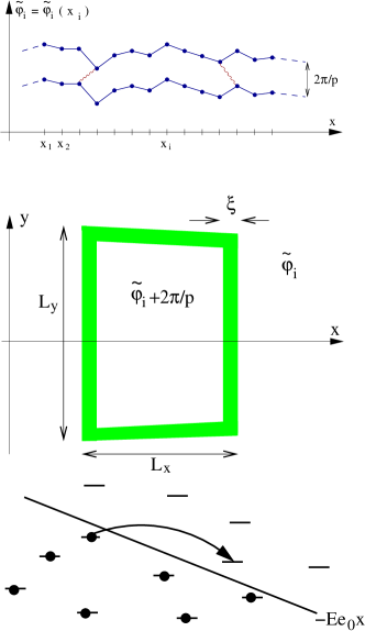
Figure 2: Upper figure: two equivalent ground states with two bifurcation sites which facilitate the formation of an instanton in nonzero external field. Middle: Top view of an almost rectangular instanton, the width of the wall corresponds to $\xi$, i.e. the distance between the grid points of the upper figure. Lower figure: Hopping process corresponding to the instanton formation, see also Fig.3 in s73 .

To calculate the surface tension we first consider a wall parallel to the $y$-axis. Such a wall - at which $m$ is changed to $m+n$, $n=\pm 1$ - has an excess energy

$$\begin{split}\frac{H_{\text{kink}}}{T}\approx\frac{1}{2\pi\xi T}\Big{\{}\big{(}\tilde{\varphi}_{i}(m+n)-\tilde{\varphi}_{i-1}(m)\big{)}^{2}-\\ -\big{(}\tilde{\varphi}_{i}(m)-\tilde{\varphi}_{i-1}(m)\big{)}^{2}\Big{\}}=\\ =\frac{2\pi}{p^{2}\xi T}\Big{\{}1-2n\big{(}\delta\alpha_{i}-[\delta\alpha_{i}]_{G}\big{)}\Big{\}}\equiv\frac{1}{pT}\sigma_{x,i}(n)\end{split}$$ (4.7)

On the rhs we introduced the surface tension of the oriented ($n=\pm 1$) wall $\sigma_{x,i}(n)\equiv\sigma\nu_{i}(n)$, $\sigma\approx{2\pi}/({p\,\xi})$ and ngd03

$$\nu_{i}(n)=1-2n\big{(}\delta\alpha_{i}-[\delta\alpha_{i}]_{G}\big{)}\,,\,\,\,\ \nu_{i}(1)+\nu_{i}(-1)=2$$ (4.8)

and hence $0\leq\nu_{i}(n)\leq 2$. Thus we find that if we proceed in $x$-direction the surface tension $\sigma_{x,i}(n)$ of a wall with a fixed orientation is fluctuating from site to site and equally distributed in the interval $0\leq\sigma_{x,i}(n)\leq 2\sigma$. If the surface tension for a $+$-wall is close to $2\sigma$ the corresponding surface tension for the minus wall is close to zero. If we consider the surface tension of an oriented wall in a typical region (i.e. we exclude for the moment regions where rare events take place) of linear extension $L_{x}\gg\xi$, then the average m-th lowest value of $\nu_{\pm}(x)$ in this region is given by $2m\frac{\xi}{L_{x}}$.

An analogous calculation can be done for the surface tension $\sigma_{y}$ if we introduce also a lattice of grid size $\xi$ in the $y$-direction. Since the disorder is frozen in time, $\delta\alpha_{i}\equiv 0$ and hence $\sigma_{y}(n)=\sigma$. Note that the value of $\sigma$ found here agrees up to a numerical constant with the surface tension obtained for the pure case in the previous section.

IV.2 Instanton action in the disordered case

To describe the decay of the metastable state - which is in the present case one of the classical ground states $\tilde{\varphi}_{i}(m)$ equation (4.5) - the functional integration in $Z_{1}$ has to include the integration over droplet configurations of the new phase $\tilde{\varphi}_{i}(m+1)$ starting with small droplets which subsequently enlarge in both $x$ and $y$-direction until the new metastable state is reached at least in a part of the $1d$ system. Since the surface tension $\sigma_{x}$ can become arbitrarily low it is obvious that the dominating droplet configurations are those bounded by walls essentially parallel to the $y$-axis. Once the saddle point (the instanton) is reached, the droplet will expand only in $y$-direction since further expansion in $x$-direction is prohibited by the high cost of leaving the wall position with extra low surface tension. The maximal extension of the droplet in $x$-direction will be denoted by $L_{x,c}$.

We will start our quantitative consideration by restricting ourselves to rectangular droplets of linear extension $L_{x}$ and $L_{y}$, respectively. The instanton action $S(L_{x},L_{y})$ is then given by

$$\begin{split}\frac{S(L_{x},L_{y})}{\hbar}\frac{pK_{\text{eff}}}{\sigma}\equiv\tilde{S}(L_{x},L_{y})=L_{x}\big{\{}2+\eta\ln\frac{L_{y}}{\xi}\big{\}}+\\ +\big{\{}\nu_{+}(x)+\nu_{-}(x+L_{x})-R_{c}^{-1}L_{x}\big{\}}L_{y}\ ,\end{split}$$ (4.9)

where we have included also the contribution of the dissipation Hida+Eckern . We will assume here that the dissipation is weak, $\eta\ll 1$. It should be noted that the dissipation favors in general a rectangular shape of the instanton even in the absence of disorder Hida+Eckern . $\nu_{\pm}(x)$ denotes the generalization of $\nu_{i}(n=\pm 1)$ to a continuum description and is a random quantity equally distributed in the interval $0\leq\nu_{\pm}\leq 2$ with a correlation length of the order $\xi$. $R_{c}$ is still given by (3.9). The functional integral corresponding to (III) takes now the form

$$\frac{Z_{1}}{Z_{0}}\sim\operatorname{Im}\int dL_{x}dL_{\tau}\,e^{-S(L_{x},L_{\tau})/\hbar}\,.$$ (4.10)

It is illustrative to consider the evaluation of (4.10) for the pure case, where $\nu_{\pm}(x)\equiv 1$, and $\eta\equiv 0$, ignoring for the moment the fact that the consideration of circular droplets is here more natural. The main contribution to (4.10) comes now from quadratic droplets since for a given area the square has the least circumference. At the saddle point $L_{x,c}=L_{y,c}=2R_{c}$ and the instanton action is $\tilde{S}_{c}=4R_{c}$. Clearly, circular droplets have a lower saddle point action $\tilde{S}_{c}=\pi R_{c}$.

In the impure case the situation is different because of the variation of the surface tension $\nu_{\pm}(x)$. The saddle point will be determined by low values of the surface tension $\nu_{+}(x)+\nu_{-}(x+L_{x})$. Since the surface tension $\nu(x)$ fluctuates on the scale $\xi$, the droplet will not - as in the pure case - expand both in the $x$- and in the $y$-direction. For the further discussion it is useful to use the parametrization $L_{x}=\Lambda\cdot l_{x}$ where $0<l_{x}\leq 1$. In an $x$-interval of extension $\Lambda$ the typical surface tension fulfills the inequality

$$2\frac{\xi}{\Lambda}\lesssim\nu_{+}(x)+\nu_{-}(x+L_{x})\equiv 2\frac{\xi}{L_{x}}\mu(x,l_{x})\lesssim 2.$$ (4.11)

For a typical region $\mu(x,l_{x})\approx\mu(l_{x})$ will not depend on the choice of $x$. As explained above $\mu(l_{x})$ is strongly fluctuating with a correlation length $\xi/\Lambda$. Since we have no detailed information about the strongly fluctuating surface tension $\mu(l_{x})$ we now minimize $S$, Eq. (4.9), with respect to the scale factor $\Lambda$ and $L_{y}$, and choosing such a value of $l_{x}$ that $\mu(l_{x})$ is of the order one. This gives the saddle point equations:

$$\begin{split}L_{x}(2+\eta\ln\frac{L_{y}}{\xi})-(2\frac{\xi}{L_{x}}\mu(l_{x})+\frac{L_{x}}{R_{c}})L_{y}=0,\\ \eta\frac{L_{x}}{L_{y}}+2\frac{\xi}{L_{x}}\mu(l_{x})-\frac{L_{x}}{R_{c}}=0.\end{split}$$ (4.12)

Note, that the second equation describes the energy conservation during tunneling. These equations have the solution

$$\begin{split}L_{x,c}^{2}=2\xi R_{c}\mu(l_{x})\frac{1+\frac{\eta}{2}\ln(\frac{eR_{c}}{\xi})}{1+\frac{\eta}{2}\ln(\frac{R_{c}}{e\xi})},\\ L_{y,c}=R_{c}\left(1+\frac{\eta}{2}\ln\left(\frac{eR_{c}}{\xi}\right)\right).\end{split}$$ (4.13)

Thus we get for the saddle point action

$$\frac{S_{c}}{\hbar}=\frac{2\sigma}{pK_{\text{eff}}}\sqrt{\mu(l_{x})\xi R_{c}}\sqrt{\left(1+\frac{\eta}{2}\ln\frac{R_{c}}{\xi}\right)^{2}-\left(\frac{\eta}{2}\right)^{2}}.$$ (4.14)

This solution becomes exact in the quasiclassical limit $K_{\rm eff}\ll 1$. For $K_{\rm eff}\lesssim 1$, there are additional fluctuations which lead to downward renormalization of the surface tension.

IV.3 Stability of the saddle point solution

Considering quadratic fluctuations around the saddle point it is easy to show that one eigenvalue is negative as it has to be the case for an instanton. The eigenvector corresponding to this eigenvalue has a small component in $x$-direction which could suggest a further growth of the droplet both in $y$- and in $x$-direction. For the further discussion it is however important to realize that the decay from the true saddle point has to follow one of the many surface tension minima inscribed in the function $\mu(l_{x})$ and which determines the saddle point value of $l_{x}$. The latter would follow from a more microscopic approach using a variation with respect to $L_{x}=\Lambda l_{x}$. Such a treatment would require the detailed knowledge of the energy landscape $\mu(l_{x})$ which is unknown. Since $\mu(l_{x})$ is of the order of one for the low surface tension valleys we conclude the for the true saddle point $l_{x,c}\equiv l_{c}$ and $\mu(l_{c})\equiv\mu_{c}$ remain unspecified, but are both of order unity. Such a decay within one energy valley can only happen if (i) the slope of $S$ in $y$-direction is negative and (ii) if

$$\frac{\partial^{2}S}{\partial L_{y}^{2}}|_{L_{y}=L_{y,c}}=-\eta\frac{L_{x}}{L_{y}^{2}}<0.$$ (4.15)

The first condition is fulfilled, as one can see from the saddle point equation for $L_{y}$. The second condition depends crucially on the existence of dissipation. Without dissipation, e.g. the emission of phonons, the decay to the new metastable state is impossible because it would violate energy conservation. In experimental systems, dissipation is always present, for example due to electron phonon coupling. The precise way in which the dissipation strength enters the final result as a prefactor is beyond the logarithmic accuracy of our present calculation. However, from a comparison with the decay rate of dissipative two level systems Weiss99 we conjecture that the decay rate is proportional to the damping strength $\eta$. The answer to the question whether an short range interacting and disordered 1D electron system has a sufficient amount of intrinsic dissipation to support a finite creep current is clearly beyond the scope of the present work.

As a final result we get for the decay rate $\Gamma(E)$ in the limit of $\eta\ll 1$, $E\ll E_{0}$ and hence for the nonlinear zero temperature conductivity $\sigma(E)$

$$\ln\Gamma(E)\sim\ln\sigma(E)\sim-2\frac{L_{x}(E)}{\xi_{\text{loc}}}\left(1+{\eta}{}\ln\frac{L_{x}(E)}{\xi}\right)$$ (4.16)

where

$$\frac{L_{x}(E)}{\xi_{\text{loc}}}\approx\sqrt{\frac{E_{0}}{E}},\,\,\,\,\,\,\,\,E_{0}=\frac{\pi\hbar v}{pKe_{0}\xi_{\text{loc}}^{2}}=\big{(}p\kappa e_{0}\xi_{\text{loc}}^{2}\big{)}^{-1}\,\,\,\,.$$ (4.17)

$L_{x}(E)$ denotes the extension of the instanton and hence the distance over which charges are tunneling in $x$-direction. $\kappa$ is the compressibility which depends on the interaction parameter $K$ (compare Appendix A). $\xi_{\text{loc}}=p^{2}\xi K_{\text{eff}}$ is the localization length of the tunneling charges, in agreement with a result of Fogler fogler02 . In fact the correlation length $\xi$ was used in Giamarchi+Schulz ; ngd03 and subsequent papers as the localization length, which is correct for intermediate $K$. In the limit $K\to 0$, $\xi$ goes over into the Fukuyama-Lee length which is a completely classical quantity. Tunneling processes are characterized by a length scale $\xi_{\text{loc}}$ which is intrinsically of quantum mechanical origin and therefore has to vanish for $\hbar\to 0$.

IV.4 Percolating instantons

Once a single instanton was formed it will expand in the $y$-direction leaving a region of linear extension $L_{x}(E)$ behind in which the phase is advanced by $2\pi/p$. Since such a configuration corresponds to a change of the phase difference of neighboring sites at the left and right boundary of this region by $\pm 2\pi/p$ one has to conclude that such an event corresponds to a transfer of a charge $2e_{0}/p$ from one boundary to the other. Many such events will happen independently at different places of the sample, each of it leads to a local transfers of charge over a typical distance $L_{x}(E)$. A current will only flow if these tunneling processes fill eventually the whole sample, see Fig. 3.

Figure 3: Phase profile $\varphi(x)$ (bold line) after several tunneling events have happened, starting from the zero field ground state characterized by the dashed line. The thin lines show different zero field ground states which follow from each other by phase shifts of $2\pi/p$. A current flows only if the instantons form a percolating path through the sample.

It is in this respect important to note that bifurcation sites (at which the original metastable state $\tilde{\varphi}_{j}(m),\forall j$ was changed to $\varphi_{j\geq i}=\tilde{\varphi}_{j}(m+n)$ ($n=\pm 1$)) are now favorable sites for a change to $\varphi_{j}=\tilde{\varphi}_{j}(m+n),\forall j$. Indeed, if the initial reduced surface tension for this pair of sites was (compare(4.7)) $\nu_{i}=\epsilon$, then we get for the surface tension between the state $\tilde{\varphi}_{j}(m+n),\forall j$ and $\varphi_{j\geq i}=\tilde{\varphi}_{j}(m+n),\varphi_{j<i}=\tilde{\varphi}_{j}(m)$

$$\begin{split}\frac{H_{\text{kink}}}{T}\approx\frac{1}{2\pi\xi T}\Big{\{}\big{(}\tilde{\varphi}_{i}(m+n)-\tilde{\varphi}_{i-1}(m+n)\big{)}^{2}-\\ -\big{(}\tilde{\varphi}_{i}(m+n)-\tilde{\varphi}_{i-1}(m)\big{)}^{2}\Big{\}}=\\ =\frac{2\pi}{p^{2}\xi T}\Big{\{}-1+2n\big{(}\delta\alpha_{i}-[\delta\alpha_{i}]_{G}\big{)}\Big{\}}.\end{split}$$ (4.18)

The reduced surface tension of the new wall is therefore

$$\nu_{i}(n)=-1+2n\big{(}\delta\alpha_{i}-[\delta\alpha_{i}]_{G}\big{)}=-\varepsilon\ ,$$ (4.19)

i.e. these sites are preferential for the formation of new instantons which will fill the gaps between already existing regions of increased $\varphi$. These considerations have a simple interpretation in terms of the charges which undergo tunneling: In the initial ground state $\tilde{\varphi}_{i}(m)$ all occupied states have energies below the Fermi level. The creation of an instanton corresponds to the transfer of a charge ($e_{0}$ for Luttinger liquids and $2e_{0}$ for CDWs) from an occupied to an unoccupied site of distance $L_{x}(E)$. The site which is unoccupied now is below the Fermi-energy and consequently its surface tension is negative.

As one can see from (4.16) the current $I\sim-\frac{1}{\pi}\langle\dot{\varphi}\rangle\sim\Gamma(E)$ shows for $E\ll E_{0}$ creep-like behavior. The calculation of the complete pre-factor of the decay rate $\Gamma$ is beyond the scope of the present paper.

IV.5 Finite temperatures

So far we assumed that the typical extension $L_{y,c}$ of the instanton in $y$-direction is much smaller than $K_{\text{eff}}/T$. However, this condition is violated for

$$\beta<\beta_{E}\equiv\frac{p}{e_{0}E\xi_{\text{loc}}}\,\,\,\,\text{or}\,\,\,\,E<E_{\beta}=\frac{p}{e_{0}\xi_{\text{loc}}\beta}.$$ (4.20)

For higher temperatures, $\beta<\beta_{E}$, the saddle point cannot be reached any more. In the limit $\beta\ll\beta_{E}$ we can proceed as in ngd03 and consider the contribution to the average current $j\sim-\frac{1}{\pi}\langle\dot{\varphi}\rangle$ from the production of droplets of the metastable states with $n=\pm 1$.This leads in the limit $\beta e_{0}EL_{x}\ll 1$ to a linear relation between $j$ and $E$. The maximal barrier is now given by $L_{y}\approx K_{\text{eff}}/T$, $L_{x}\approx L_{x}(E_{\beta})$ which gives a linear conductivity

$$\sigma(T)\sim\exp\big{\{}-\text{const.}\sqrt{\hbar\omega_{p}\beta}/K_{\text{eff}}\big{\}}\,.$$ (4.21)

Here, $T=\pi\kappa a/\beta$ where $\beta$ is the inverse temperature, and we introduced the pinning frequency $\omega_{p}$ by

$$\omega_{p}=\frac{\pi pv_{\text{eff}}}{\xi}.$$ (4.22)

The result (4.21) can be also written in the form

$$\sigma(T)\sim\exp\big{\{}-\text{const.}\sqrt{\beta/(\kappa\xi_{\text{loc}})}\big{\}}.$$ (4.23)

where we used the compressibility $\kappa$ defined in the Appendix. Note that $\kappa$ depends on the interaction parameter $K$. Equation (4.23) is the natural extension of the Mott variable range hopping result to short range interacting electrons. A long range Coulomb interaction leads to a logarithmic correction in Eq. (4.23), see teber_fogler_shklovskii . The additional logarithmic correction due to a dissipative damping of the tunneling action by electronic degrees of freedom teber_fogler_shklovskii is only relevant for strong pinning, whereas in the situation of weak pinning this correction is absent as all electronic degrees of freedom are localized and cannot dissipate energy.

IV.6 Rare events

So far we considered typical instantons. The question arises what is the influence of regions in which the lowest surface tension is untypically large? The question was addressed for nonzero temperatures Kurkijarvi ; SerotaKaliaLee ; RaikhRuzin . We proceed in a similar manner. The regions with large surface tension will lead to a lower tunneling probability and hence act as a weak link. We may first ask the question: what is the largest distance $x_{m}$ between two consecutive sites of surface tension $\nu_{i}\leq\nu_{0}$ in a sample of length $L_{0}$? These sites are randomly distributed along the sample of length $L_{0}$. Their concentration is given by

$$n_{0}=\nu_{0}/\xi\,.$$ (4.24)

The probability distribution for the separation $x$ between such consecutive sites is

$$p_{0}(x)=n_{0}e^{-n_{0}x}\,.$$ (4.25)

The number of sites with $\nu_{i}<\nu_{0}$ has the average $L_{0}n_{0}$ and a standard deviation $\sqrt{L_{0}n_{0}}$. Therefore, the largest separation $L_{x,m}$ between such sites can be found from

$$L_{0}n_{0}\int\limits_{L_{x,m}}^{\infty}dx\,p_{0}(x)\sim 1\,,$$ (4.26)

where the integral represents the probability that the given pair of neighboring sites has the separation exceeding $L_{x,m}$. Using Eqs. (4.24) and (4.25), we find:

$$\nu_{0}=\frac{\xi}{L_{x,m}}\ln\left(L_{0}\frac{\nu_{0}}{\xi}\right)\approx\frac{\xi}{L_{x,m}}\ln\left(\frac{L_{0}}{L_{x,m}}\right)\,.$$ (4.27)

Comparing this equation with (4.11) we see that in the region considered $\mu(x,l_{x})$ is of the order $\ln(L_{0}/L_{x,m})$ instead of order one as in the typical regions. Combining this result with the saddle point equations (4.12) we find that we have use the replacement

$$\mu(l_{x})\rightarrow\mu(l_{x})\ln(L_{0}/\sqrt{\xi R_{c}})$$ (4.28)

in (4.13) and the subsequent formulas. Since it is this weak link which will control the total current ,the main exponential dependence of the current is given by

$$\ln I\sim-2\sqrt{\frac{E_{0}}{E}}\sqrt{\ln\left(\frac{L_{0}}{\xi_{\text{loc}}}{\sqrt{\frac{E}{E_{0}}}}\right)}\,.$$ (4.29)

We may now consider the influence of this weakest link on the conductivity at finite temperatures. We found before that the nonlinear conductivity crosses over to a linear behavior when the extension of the instanton in $y$-direction reaches $K_{eff}/T=L_{y,c}\approx R_{c}$. This relation is not affected by the value of the surface tension as can be seen from (4.13). We have therefore to use the same replacement $E\rightarrow E_{\beta}$ as for the typical instantons but take into account the extra factor in (4.29), which gives for the resistance of the the sample of length $L_{0}$

$$\ln(R_{m}/R_{0})\sim\sqrt{\frac{\beta}{\kappa\xi_{\rm loc}}}\sqrt{\ln\left(L_{0}\sqrt{\frac{\kappa}{\beta\xi_{\rm loc}}}\right)}\,.$$ (4.30)

Finally we mention that for exponentially large samples $L_{0}\sim\xi e^{R_{c}/\xi}$ there are weak links with surface tension $\nu_{0}$ of the order one. In this case the tunneling probability is $\ln\Gamma(E)\sim E_{0}/E$. A similar crossover with respect to the sample length was found in Refs. SerotaKaliaLee, ; RaikhRuzin, for linear conductivity in 1d in the case of nonzero temperature.

V Shklovskii and Mott Variable range hopping

In this Section we give a brief account of the derivation of Shklovkii’s zero temperature nonlinear hopping conductivity which was done for three dimensions s73 . Its extension to general dimensions $d$ is straightforward. All electrons are assumed to be localized over a distance of the order of the localization length $\xi_{\text{loc}}$. An electron can be transferred from a filled to an empty site separated by a distance $L_{x}$ without absorption of a phonon provided the difference between the difference of the energies of the states does not exceed $e_{0}EL_{x}$. If we denote the density of states (per energy and unit length) by $g(\cal{E})$, the number of states states with energy smaller than $e_{0}EL_{x}$ accessible by a jump over the spatial distance $L_{x}$ is given by $g({\cal E}_{F})\cdot e_{0}EL_{x}^{d+1}\gtrsim 1$. $\cal{E}_{F}$ denotes the Fermi energy. The minimal distance for the tunneling is therefore given $L_{x,c}\approx\big{(}e_{0}Eg({\cal E}_{F})\big{)}^{-1/(d+1)}$. The probability for an electron to jump over a distance $L_{x,c}$ is $P(L_{x})\sim e^{-2L_{x,c}/\xi_{\text{loc}}}\sim I$ and hence we get for the nonlinear current voltage relation

$$I(E)\sim e^{-\big{[}{E_{0}}/{E}\big{]}^{1/(d+1)}},\,\,\,E_{0}=\left(\frac{2}{\xi_{\text{loc}}}\right)^{d+1}(e_{0}g({\cal E}_{F}))^{-1}\ .$$ (5.1)

This result agrees with our findings (4.16) in $d=1$ dimension in the noninteracting case $K=1$.

Indeed, the one-particle density of states at the Fermi level can be written as

$$g({\cal E}_{F})=\frac{1}{L_{0}}\sum\limits_{k}\delta({\cal E}_{F}-\epsilon_{k})\,,$$ (5.2)

where $\epsilon_{k}$ are the energies of the eigenstates of the Hamiltonian describing noninteracting electrons, and $L_{0}$ is the system size. At zero temperature, the particle density $\rho$ can be expressed as

$$\rho(\mu)=\frac{1}{L_{0}}\sum\limits_{k}\Theta({\cal E}_{F}-\epsilon_{k})\,,$$ (5.3)

and hence $\kappa\equiv\partial\rho/\partial\mu=g(\mu)$ for $\mu={\cal E}_{F}$.

In the case of finite temperatures when $e_{0}E\xi_{\text{loc}}\beta<1$ the number of reachable sites is determined by thermal activation Mott69 ; ahl71 . Indeed, the number of these sites located in a volume $L_{x}^{d}$ and the energy interval $\Delta E$ is given by $g({\cal E}_{F})\Delta EL_{x}^{d}\gtrsim 1$. The hopping probability is then to be determined from the maximum of

$$P(L_{x})\sim e^{-2L_{x,c}/\xi_{\text{loc}}}e^{-\beta/(g({\cal E}_{F})L_{x}^{d})}\ ,$$ (5.4)

which gives

$$L_{x,\beta}=\Big{(}\frac{\beta d\xi_{\text{loc}}}{2g({\cal E}_{F})}\Big{)}^{1/(d+1)}\,,$$ (5.5)

and hence for the current

$$I\sim E\cdot\exp\Big{[}{-\frac{2(d+1)}{d}\Big{(}\frac{\beta d}{2g({\cal E}_{F})\xi_{\text{loc}}^{d}}\Big{)}^{1/(d+1)}}\Big{]}\,.$$ (5.6)

Thus there is a crossover from a nonlinear current voltage relation at low temperatures $\beta>\beta_{E}\equiv(e_{0}E\xi_{\text{loc}})^{-1}$ to a linear relation at higher temperatures. The result (5.6) agrees for $K=1$ again with our result (4.21).

VI The influence of Coulomb interaction

Efros and Shklovskii Efros_Shklovskii considered the influence of the Coulomb interaction on Mott variable range hopping. The Coulomb repulsion leads in dimensions $d>1$ to a suppression of the density of states close to the Fermi energy, $g({\cal E})\sim|{\cal E-E}_{F}|^{d-1}$, which changes the exponent $1/(d+1)$ in (5.1) and (5.6) to $1/2$ in all dimensions. This can be seen as follows:

To calculate the density of states in a system with Coulomb interaction we first consider deviations from the ground state. For any pair of localized states close to the Fermi surface the transfer of an electron from am occupied site ${\bf r}_{i}$ of energy ${\cal E}_{i}<{\cal E}_{F}$ to an empty site ${\bf r}_{j}$ of energy ${\cal E}_{j}>{\cal E}_{F}$ the net change of energy has to be positive

$$\Delta{\cal E}={\cal E}_{j}-{\cal E}_{i}-\frac{e_{0}^{2}}{\epsilon_{s}\mid{\bf r}_{i}-{\bf r}_{j}\mid}>0.$$ (6.1)

Here $\epsilon_{s}$ denotes the dielectric constant. Let us now assume that we consider all energy levels with $\mid{\cal E}_{i}-{\cal E}_{F}\mid<{\tilde{\cal E}}$. Apparently, they have to fulfill the inequality (6.1) which gives

$$\mid{\bf r}_{i}-{\bf r}_{j}\mid\gtrsim\frac{e_{0}^{2}}{\epsilon_{s}\tilde{\cal E}}.$$ (6.2)

Hence the donor concentration $n({\tilde{\cal E}})$ cannot be larger than $n({\tilde{\cal E}})\lesssim\big{(}\frac{e_{0}^{2}}{\epsilon_{s}\tilde{\cal E}}\big{)}^{-d}$, from which we find for the density of states $g(\tilde{\cal E})=\frac{dn(\tilde{\cal E})}{d{\tilde{\cal E}}}\approx{\tilde{\cal E}}^{d-1}\epsilon_{s}^{d}/e_{0}^{2d}$. Thus there is no change in the density of states in $d=1$ dimensions. A slightly more refined calculation gives a logarithmic correction to the density of states which give logarithmic modifications of in the exponents of (5.1) and (5.6)teber_fogler_shklovskii ; teber .

We consider now the influence of long range Coulomb interaction. In the Fourier transformed action (2.8) $k^{2}|\varphi_{k}|^{2}$ is replaced by $k^{2}(1+{\cal C}\ln(k_{F}/k))|\varphi_{k}|^{2}$ where the dimensionless prefactor ${\cal C}=\frac{2\pi e_{0}^{2}K}{\hbar v\epsilon_{s}}=\frac{2\pi^{2}e^{2}_{0}\kappa}{\epsilon_{s}}$ measures the relative strength of the Coulomb interaction. Fluctuations of $\varphi$ are now reduced leading to a suppression of the transition to the delocalized superconducting phase. The effect of the Coulomb interaction in the localized phase is weak and we have still a flow of our coupling parameter $u$ to large values. Following our considerations of Section IV we have next to construct the exact ground state in the presence of Coulomb interaction. Because of its nonlocal character, Eq. (4.5) is not longer the true ground state. However, it is clear that any configuration which deviates from the ground state has to increase the energy. We consider now the instanton as such a configuration. The effective instanton action is now given by

$$\begin{split}\frac{S(L_{x},L_{y})}{\hbar}\frac{pK_{\text{eff}}}{\sigma}=L_{x}\big{\{}2+\eta\ln\frac{L_{y}}{\xi}\big{\}}+\\ +\big{\{}\big{(}{\mu}(x,l_{x})-{\tilde{\cal C}\big{)}\frac{\xi}{L_{x}}}-\frac{L_{x}}{R_{c}}\big{\}}L_{y}.\end{split}$$ (6.3)

Here ${\mu}$ denotes now the surface tension in the presence of the Coulomb interaction and there is an additional contribution $\sim\tilde{\cal C}\sim{\cal C}$ from the Coulomb interaction between the surfaces. Since we consider deviations from the ground state, ${\mu}(x,l_{x})-{\tilde{\cal C}}$ has to be positive. It is therefore tempting to assume that this difference scales as ${\mu}(x,l_{x})-{\tilde{\cal C}}\approx{\mu}_{\cal C}(l_{x})$ and the results of Section IV apply with ${\mu}(l_{x})$ replaced by ${\mu}_{\cal C}(l_{x})$, in complete agreement with the consideration for the case without long-range interactions. Thus, the Coulomb interaction does not change the power law dependence of the the results (4.16) and (4.23) on $E$ and $\beta$. There is a logarithmic corrections to $\mu_{\cal C}(l_{x})$ due to long range Coulomb interactions teber which is beyond the accuracy of the present calculation.

VII Delocalization in strong fields

For our discussion of quantum creep in 1d electronic systems the presence of dissipation was essential. A possible nonlinear I-V characteristic in noninteracting electron systems without dissipation was discussed by Prigodin Prigodin80 and others Soukoulis+83 ; DeSiSo84 ; Kirkpatrick86 ; PriAl89 . This nonlinearity is due to a field dependent delocalization of electronic wave functions. To understand whether this mechanism possibly interferes with the quantum creep discussed in section IV., we briefly review its derivation and discuss a generalization to short range interacting electron systems afterwards.

The disordered potential (2.4) consists of a series of delta function scatterers of strength $u_{0}$ placed at irregular positions $x_{i}$ with a mean density $n_{\rm imp}$. A free electron incident with energy $\cal{E}$ on one of these scatterers is reflected back with a probability

$$R({\cal E})=\Big{[}1+\frac{2{\cal E}\hbar^{2}}{mu_{0}^{2}}\Big{]}^{-1}\ .$$ (7.1)

Neglecting localization effects for the moment, the energy dependent mean free path is given by $\ell({\cal E})={R^{-1}({\cal E})}{n^{-1}_{\rm imp}}$. In the presence of an external electric field, the electron kinetic energy becomes position dependent according to ${\cal E}(x)={\cal E}_{0}+eEx$, leading to a position dependent mean free path

$$\ell(x)=\left[1+\frac{2\hbar^{2}}{mu_{0}^{2}}({\cal E}_{0}+e_{0}Ex)\right]\frac{1}{n_{\rm imp}}\ \$$ (7.2)

for noninteracting electrons. In one-dimensional systems, the localization length $\xi_{\rm loc}$ is approximately equal to the mean free path Berezinskii73 . The equality between mean free path and localization length is valid even in the presence of an electric field, as the additional phase shift that the electron acquires as it moves along the field is canceled out on the return trip counter to the field Prigodin80 . Thus, the energy dependence of the backscattering probability of an individual scatterer gives rise to a position dependent localization length $\xi_{\rm loc}(x)\sim\ell(x)$.

Without applied external field, a localized electronic state centered around a position $x_{0}$ is characterized by an exponentially decaying wave function envelope $\Psi(x)\sim\exp(-|x-x_{0}|/\xi_{\rm loc})$. In the presence of an external field, the localization length acquires a position dependence. The electron kinetic energy changes on a length ${\cal E}_{0}/e_{0}E$. If the localization length is much smaller than this length scale, $\xi_{\rm loc}\ll{\cal E}_{0}/e_{0}E$, the localization length varies slowly in space, and the wave function envelope is given by Kirkpatrick86

$$\Psi(x)\sim\left\{\begin{array}[]{ll}e^{-(x_{0}-x)/\xi_{\rm loc}(x_{0})}&,x<x_{0}\\ e^{-\int_{x_{0}}^{x}d\tilde{x}\frac{1}{\xi_{\rm loc}(\tilde{x})}}&,x>x_{0}\end{array}\right.\ \ .$$ (7.3)

Using the explicit position dependence of the mean free path given in (7.2), one finds that the envelope decays asymptotically as a power

$$\Psi(x)\sim\left[1+\frac{(x-x_{0})eE}{{\cal E}_{0}}\right]^{-\frac{mn_{\rm imp}u_{0}^{2}}{2e_{0}E\hbar^{2}}}$$ (7.4)

The state is only localized if it is normalizable, i.e. the integral over the envelope squared

$$\int_{-\infty}^{\infty}dx\;\Psi^{2}(x)<\infty$$ (7.5)

must be finite. The wave function is only normalizable if the envelope decays faster than $1/\sqrt{x}$ or if the electric field is weaker than the critical electric field

$$E_{c}=\frac{mn_{\rm imp}u_{0}^{2}}{e_{0}\hbar^{2}}\ .$$ (7.6)

This calculation underestimates the exact result Prigodin80 by a factor of two. We want to compare this critical field to the crossover field $E_{0}=\frac{\pi v\hbar}{\xi_{\rm loc}^{2}e_{0}}$ obtained from Eq. (4.16) for the creep current. Using the relation $\xi_{\rm loc}\approx\frac{2\hbar^{2}{\cal E}_{F}}{mu_{0}^{2}n_{\rm imp}}$ valid for noninteracting electrons, the crossover field Eq. (7.6) can be rewritten as $E_{c}=E_{0}k_{F}\xi_{\rm loc}\gg E_{0}$. From this relation one sees that the instanton mechanism is effective already at fields which are parametrically smaller than the critical field for delocalization.

If the point scatterers are not of delta-function type but characterized by a finite interaction range instead, even an arbitrarily weak external electric field will lead to delocalization on long length scales as the backscattering probability drops significantly for electron wave vectors larger than the inverse potential range.

How can this argument be generalized to short range interacting electrons? If the particle density is spatially homogeneous, the kink kinetic energy far from the center of localization is much larger than the Fermi energy of the interacting system and the kink should essentially behave like a free particle. In this case, the kink wave function would stay localized for fields below the threshold value (7.6), and the power law tail of the kink wave function could possibly enhance the tunneling current derived in Sec. IV. Alternatively, the charge density may be locally in equilibrium with the electro-chemical potential. In this situation, both the particle density and the Fermi wave vector are position dependent. Assuming that the free electron relation ${\cal E}_{F}=\frac{\hbar^{2}k_{F}^{2}}{2m}$ is at least approximately valid, the Fermi wave vector acquires a position dependence

$$k_{F}(x)=\sqrt{\frac{2m}{\hbar^{2}}({\cal E}_{0}+eEx)}\ \ .$$ (7.7)

Expressing the cutoff as $\Lambda=k_{F}$, the localization length depends on the Fermi wave vector according to

$$\xi_{\rm loc}\propto k_{F}^{-1}\left(k_{F}L_{\rm FL}\right)^{\frac{1}{(1-K/K_{c})}}\ ,$$ (7.8)

where the classical Fukuyama-Lee length $L_{\rm FL}$ is independent of $k_{F}$. For a noninteracting system, $K/K_{c}=2/3$ and one retrieves the dependence $\xi_{\rm loc}\sim k_{F}^{2}$. For general $K$, the position dependence of the localization length is

$$\xi_{\rm loc}(x)\propto\left[\frac{2m}{\hbar^{2}}({\cal E}_{0}+eEx)\right]^{\frac{K}{2(K_{c}-K)}}\ L_{\rm FL}^{\frac{K_{c}}{K_{c}-K}}\ .$$ (7.9)

Accordingly, the wave function envelope decays as a stretched exponential $\exp\left(-{\rm const}\;x^{\frac{K_{c}-3K/2}{K_{c}-K}}\right)$ for $K<1$ and does not decay to zero at all for $K>1$. The argument leading to this result contains approximations which may be correct only qualitatively. For this reason, we only draw the conclusion that the delocalizing effect of an external field is weakened by repulsive short range interactions and enhanced by attractive ones. In order to determine whether the critical field strength $E_{c}$ indeed has a discontinuity when varying $K$ across one a more sophisticated calculation is necessary.

In conclusion, the delocalization mechanism studied in this paragraph does not seem to interfere with the creep current described by formula Eq. (4.25) for the case of repulsive short range interactions.

VIII Conclusion

In the present paper we extended Mott’s and Shklovskii’s approach for 1D variable range hopping conductivity to short range interacting electrons in charge density waves and Luttinger liquids using an instanton approach. Following the recent paper ngd03 , we calculated the quantum creep of charges at zero temperature and the linear conductivity at finite temperatures for these systems. The main results of the paper are equations (4.16) for zero temperature and (4.23) for nonzero temperatures, respectively.

In our approach the quantum effects are weak but essential for the transport. An applied electric field renders all classical ground states metastable, and the motion between ground states along the electric field occurs via quantum tunneling. We were interested in the effect of the collective pinning by weak impurities, which always localizes a 1D system with repulsive short range interactions on a sufficiently large length scale. The presence of disorder favors the charge transport: the corresponding pure system has an excitation energy gap.

In the case with disorder, the notion of the materialization is different from that in the pure case. The disordered system is intrinsically inhomogeneous, so that the transport occurs as a sequence of local materialization events. In the fermion picture these correspond to separate hops whose positions and lengths depend on the disorder configuration. At zero temperature, the typical hop length depends on the electric field $E$ and is given by $L_{x}=\xi_{\rm loc}\sqrt{E_{0}/E}$. In this regime, the conductivity reads: $\sigma\propto\exp(-\sqrt{E_{0}/E})$. Quantum creep takes place for $E\ll E_{0}$. The results can be expressed in terms of the localization length and the compressibility.

We compared the electric field $E_{0}$ with the threshold field $E_{c}$ found in Refs. Prigodin80, ; Soukoulis+83, ; DeSiSo84, ; Kirkpatrick86, ; PriAl89, : $E_{0}\sim E_{c}/(k_{F}\xi_{\rm loc})\ll E_{c}$, therefore we expect that our creep conductivity result is valid.

We demonstrated that the inclusion of the dissipative term in the action is necessary to find an unstable mode in the functional integral. Besides, the dissipative bath takes into account the possibility of inelastic processes and ensures the energy conservation. The question about the energy balance does not appear in the treatment of the pure system where the gain in the electric field energy is spent on the increase of the kinetic energy of departing kinks.

However, for weak dissipation, our result for the exponent in the quantum creep regime only weakly depends on the dimensionless dissipative coefficient $\eta$. This feature can certainly change as one crosses over to the nonzero temperature regime with linear conductivity.

The effect of the Coulomb interaction in 1D was shown to be irrelevant. It destroys the delocalization transition, but it is not expected to change much in the phase already localized by the disorder.

Appendix A

Here we recall several relations for the bosonic representation of $1d$ spinless fermions. In a one-dimensional system of short range interacting fermions, the excitations can be understood as density fluctuations of bosonic nature. Following Ref. KaneFisher, , we define the compressibility as the derivative of the particle density with respect to the chemical potential: $\kappa=\partial\rho/\partial\mu$. Correspondingly, the elastic energy density is given by $(\delta\rho)^{2}/(2\kappa)$.

Using expression (2.1) for the long-wavelength deviation of the density $\delta\rho=\partial_{x}\varphi/\pi$ from $\rho_{0}$, we can rewrite the elastic energy in the form of the second term in the Hamiltonian (2.7) if

$$\kappa^{-1}=\frac{\pi\hbar v}{K}\,,\quad{\rm i.e.}\quad\frac{v}{K}=\frac{1}{\pi\hbar\kappa}\,.$$ (A.1)

The last combination is usually denoted by $v_{N}$.

As both pressure and chemical potential depend only on the ratio $N/V$, one can derive a relation between the conventional isothermal compressibility AGD

$$\tilde{\kappa}=-\frac{1}{V}\frac{\partial V}{\partial P}=\rho^{-2}\frac{\partial\rho}{\partial\mu}=\frac{\kappa}{\rho^{2}}$$ (A.2)

and the above defined $\kappa$. We should note that he compressibility in Ref. Haldane, was defined as $\rho^{2}(\partial\mu/\partial\rho)$ which is the inverse of the conventional thermodynamic isothermal compressibility $\tilde{\kappa}$.

The kinetic energy is relevant for the description of dynamical (quantum) phenomena. In a less rigorous way we may argue that the first term in Hamiltonian (2.7) has its origin in a sum of single-particle kinetic energies $p^{2}/(2m)$, where $p$ is the momentum conjugate to the displacement, which is proportional to $\varphi$, and $m$ is the effective mass. Then, using commutator (2.3) and the mentioned proportionality relations, we obtain a relation between the coefficient in the Hamiltonian and fermionic quantities

$$Kv=\frac{\pi\hbar\rho_{0}}{m}\,.$$ (A.3)

This quantity is often referred to as $v_{J}$.

Thus, the parameters of the bosonized Hamiltonian, the stiffness $K$ and the phason velocity, can be expressed in terms of the fermion system parameters Haldane :

$$K=\pi\hbar\sqrt{\frac{\rho_{0}\kappa}{m}}\,,\qquad v=\sqrt{\frac{\rho_{0}}{m\kappa}}\,.$$ (A.4)

In the $g$-ology approach, the compressibility and the effective mass are found as

$$\kappa=\frac{2\pi}{\pi\hbar(2\pi v_{F}+g_{4}+g_{2})},\qquad m=\frac{2\pi p_{F}}{2\pi v_{F}+g_{4}-g_{2}}\,,$$ (A.5)

with the Fermi momentum $p_{F}=\pi\hbar\rho_{0}$. Repulsion ($K<1$) usually corresponds to a smaller compressibility and a larger sound (phason) velocity.

Appendix B

In this appendix, we justify our choice of an Ohmic dissipation in Eq. (3.19) and argue that it captures the generic features of more general, and possibly material specific, dissipative mechanisms. Coupling of the 1d electron systems to one- or higher dimensional phonon degrees of freedom is the obvious candidate for the realization of dissipation. This mechanism is extensively discussed in the literature on Mott variable range hopping, see BoBr85 for a review. The action for a bath with arbitrary dispersion relation and coupling to the electron system is given by

$${S_{\rm dis}\over\hbar} = {1\over\Omega_{\rm ph}}\sum_{\alpha}\int_{\beta/2}^{\beta/2}d\tau\left[{1\over 2}c_{\alpha}(\tau)\left(-{\partial^{2}\over\partial_{\tau}^{2}}+\omega_{\alpha}^{2}\right)c_{\alpha}(\tau)+\right.$$ (B.1)

$$\left.\int{dq\over 2\pi}\varphi(-q,\tau)U(q)\Phi_{\alpha}(q)c_{\alpha}(\tau)\right]\ \ .$$

Here, the $c_{\alpha}$ are bosonic bath degrees of freedom with eigenfunctions $\Phi_{\alpha}(q)$, eigenfrequencies $\omega_{\alpha}$, a coupling $U(q)$ to the electronic degrees of freedom, and $1/\Omega_{\rm ph}$ is the volume element for one eigenstate in the $\alpha$–representation. After integrating out the bath degrees of freedom, one finds the dissipative term

$${S_{\rm dis}\over\hbar}=-T\sum_{\omega_{n}}\int\!{dqdq^{\prime}\over(2\pi)^{2}}\varphi(q)K(q,q^{\prime};\omega_{n})\varphi(q^{\prime})$$ (B.2)

with the kernel

$$K(q,q^{\prime};\omega_{n})={U(q)U(q^{\prime})\over 2\Omega_{\rm ph}}\sum_{\alpha}{\Phi_{\alpha}(-q)\Phi_{\alpha}(-q^{\prime})\over\omega_{n}^{2}+\omega_{\alpha}^{2}}\ .$$ (B.3)

The precise structure of the kernel $K$ depends on the dispersion relation $\omega_{\alpha}$, the wave functions $\Phi_{\alpha}(q)$, and the coupling $U(q)$ of the dissipative bath. For the instanton calculation in section IV we have used a generic Ohmic dissipation $K(q,q^{\prime};\omega_{n})=\eta\delta(q+q^{\prime})|\omega_{n}|$ giving rise to a term $\eta L_{x}\ln L_{y}$ in the instanton action. For a material specific choice of parameters one may not find this Ohmic dissipation, but instead a general dependence $\eta F(L_{x},L_{y})$. In the following, we will argue that (i) for a weak coupling to the bath, one finds only a logarithmic dependence of the instanton action on the external electric field and hence no change of the exponential field dependence in Eq.4.16 and that (ii) $S_{\rm dis}$ generally has a negative second derivative with respect to $L_{y}$.

For a weak coupling to the bath, the dominant process will be the hop of a kink accompanied by the emission of one excitation of the bath. This process is described by a first order Taylor expansion

$$e^{-{\eta\over\hbar}F(L_{x},L_{y})}\!\approx\!1\!-\!{\eta\over\hbar}F(L_{x},L_{y})=1\!-\!{\eta\over\hbar}e^{\ln F(L_{x},L_{y})}.$$ (B.4)

The zero order term does not make any contribution to the imaginary part of the partition function $Z_{1}$. In the spirit of such a Taylor expansion, one typically finds that the preexponential factor for Mott variable range hopping conductivity is proportional to the square of the electron bath coupling and in our notation proportional to $\eta$. According to this expansion, the instanton action contains a term $\ln F(L_{x},L_{y})$ and depends via $L_{x}$, $L_{y}$ only in a logarithmic fashion on the external electric field.

To illustrate our claim (ii) that generally ${\partial^{2}F(L_{x},L_{y})\over\partial L_{y}^{2}}<0$, we consider the specific example of a local coupling of the 1d electron system to 1d acoustic phonons, i.e. the general index $\alpha$ corresponds to momentum $q$, $U(q)\propto U_{0}q^{2}$ (here $U_{0}$ is the dimensionless electron-phonon coupling constant), $\omega_{\alpha}=v_{\rm ph}q$. For an instanton with $L_{x}\ll{v_{\rm ph}\over v}L_{y}$ one finds

$${S_{\rm dis}\over\hbar}\propto{\rm const.}-{L_{x}^{2}\over L_{y}^{2}}{U_{0}^{2}v^{2}\over v_{\rm ph}^{2}}$$ (B.5)

and hence a negative second derivative with respect to time.

References

- (1) T. Giamarchi, Quantum Physics in One Dimension (Oxford Univ. Press, 2003).
- (2) G. Grüner, Density Waves in Solids (Addison-Wesley, New York, 1994).
- (3) T. Giamarchi and H. J. Schulz, Phys. Rev. B 37, 325 (1988).
- (4) C. L. Kane and M. P. A. Fisher, Phys. Rev. B 46, 15233 (1992).
- (5) A. Furusaki and N. Nagaosa, Phys. Rev. B 47, 4631 (1993).
- (6) D. Yue, L. I. Glazman, and K. A. Matveev, Phys. Rev. B 49, 1966 (1994).
- (7) A. I. Larkin and P. A. Lee, Phys. Rev. B 17, 1596 (1978).
- (8) A. M. Finkelstein Zh. Eksp. Teor. Fiz. 84, 166 (1983) [ Sov. Phys. JETP 57, 97 (1983)]; Z. Phys. B 56, 189 (1984); C. Castellani, C. DiCastro, B.G. Kotliar, and P. A. Lee, Phys. Rev. Lett. 56, 1179 (1986).
- (9) N. F. Mott and W. D. Twose, Adv. Phys. 10, 107 (1961).
- (10) D. Belitz and T. R. Kirkpatrick, Rev. Mod. Phys. 66, 261-380, (1994).
- (11) A. Glatz and T. Nattermann, Phys. Rev. Lett. 88, 256401 (2002).
- (12) A. Glatz and T. Nattermann, Phys. Rev. B 69, 115118 (2004).
- (13) N. F. Mott, Phil. Mag. 19, 835 (1969).
- (14) V. Ambegaokar, B. I. Halperin, and J. S. Langer, Phys. Rev. B 4, 2612 (1971).
- (15) B. I. Shklovskii and A. L. Efros, Electronic Properties of Doped Semiconductors ( Springer Series in Solid State Sciences 45, Springer, Berlin 1984).
- (16) V. L. Berezinskii, Zh. Eksp. Teor. Fiz. 65, 1251 (1973) [Sov. Phys. JETP 38, 620 (1973)].
- (17) E. Abrahams, P. W. Anderson, D. C. Licciardello, and T. V. Ramakrishnan, Phys. Rev. Lett. 42, 673 (1979).
- (18) R. Oppermann and F. Wegner, Z. Phys. B 34, 327 (1979).
- (19) D. Vollhardt and P. Wölfle, Phys. Rev. Lett. 45, 842 (1980); Phys. Rev. B 22, 4666 (1980).
- (20) F. D. M. Haldane, Phys. Rev. Lett. 47, 1840 (1981).
- (21) L. B. Ioffe and V. M. Vinokur, J. Phys. C 20, 6149 (1987).
- (22) T. Nattermann, Europhys. Lett. 4, 1241 (1987).
- (23) T. Nattermann, T. Giamarchi, and P. Le Doussal Phys. Rev. Lett. 91, 056603 (2003).
- (24) J. S. Langer, Ann. Phys. (N.Y.) 41, 108 (1967).
- (25) L. S. Schulman, Techniqes and Applications of Path Integration (J. Wiley & Sons, New York, 1981).
- (26) G. t’Hooft, Phys. Rev. Lett. 37, 8 (1976).
- (27) S. Coleman, Phys. Rev. D 15, 2929 (1977); C. G. Callan and S. Coleman, Phys. Rev. D 16, 1762 (1977); S. Coleman, Aspects of symmetry, Selected Erice lectures (Cambridge Univ. Press, Cambridge, 1985).
- (28) K. Maki, Phys. Rev. Lett. 39, 46 (1977); K. Maki, Phys. Rev. B 18, 1641 (1978).
- (29) R. P. Feynman and A. R. Hibbs, Quantum Mechanics and Path Integrals (McGraw-Hill, New York, 1965).
- (30) A.O. Caldeira and A.J. Leggett, Phys. Rev. Lett. 46, 211 (1981).
- (31) K. Hida and U. Eckern, Phys. Rev. B 30, 4096 (1984).
- (32) A. I. Larkin and Yu. N. Ovchinikov, J. Stat. Phys. 41, 425 (1985).
- (33) H. Kleinert, Path Integrals in Quantum Mechanics, Statistics and Polymer Physics (World Scientific, Singapore, 1995).
- (34) U. Weiss, Quantum Dissipative Systems (World Scientific, Singapore, 1999).
- (35) I. V. Gornyi, A. D. Mirlin, and D. G. Polyakov, Phys. Rev. Lett. 95, 046404 (2005), cond-mat/0407305.
- (36) B. I. Shklovskii, Fiz. Tekh. Poluprovod. 6, 2335 (1972) [Sov. Phys.–Semicond. 6, 1964 (1973)].
- (37) A. L. Efros and B.I. Shklovskii, J. Phys. C8, L49 (1975).
- (38) V. N. Prigodin, Zh. Eksp. Teor. Fiz. 79, 2338 (1980) [Sov. Phys. JETP 52, 1185 (1980)].
- (39) C. M. Soukoulis, J. V. Jose, E. N. Economou, and P. Sheng, Phys. Rev. Lett. 50, 764 (1983).
- (40) F. Delyon, B. Simon, and B. Souillard, Phys. Rev. Lett. 52, 2187 (1984).
- (41) T. R. Kirkpatrick, Phys. Rev. B 33, 780 (1986).
- (42) V. N. Prigodin and B. L. Altshuler, Phys. Lett. A 137, 301 (1989); V. I. Perel’ and D. G. Polyakov, Sov. Phys. JETP 59, 204 (1984).
- (43) U. Schultz, J. Villain, E. Brezin, and H. Orland, J. Stat. Phys. 51, 1 (1988).
- (44) H. W. Diel, D. M. Kroll, and H. Wagner, Z. Phys. B 36, 329 (1980).
- (45) M. M. Fogler, Phys. Rev. Lett. 88, 186402 (2002).
- (46) R. A. Serota, R. K. Kalia, and P. A. Lee, Phys. Rev. B 33, 8441 (1986).
- (47) M. E. Raikh and I. M. Ruzin, Sov. Phys. JETP 68, 642 (1989) [Zh. Exp. Teor. Fiz. 95, 1113 (1989)].
- (48) M. M. Fogler, S. Teber and B. I. Shklovskii, Phys. Rev. B 69, 35413(2004).
- (49) S. Teber, Eur. Phys. J. B 49, 289 (2006), cond-mat/0404449.
- (50) J. Kurkijärvi, Phys. Rev. B 5, 922 (1973).
- (51) A. A. Abrikosov, L. P. Gorkov, and I. E. Dzyaloshinski, Methods of Quantum Field Theory in Statistical Physics, Prentice Hall (1963).
- (52) H. Böttger and V.V. Bryskin, Hopping Conduction in Solids, VCH Weinheim (1985).