Quantum transport of non-interacting Fermi gas in an optical lattice combined with harmonic trapping

Abstract

We consider a non-interacting Fermi gas in a combined harmonic and periodic potential. We calculate the energy spectrum and simulate the motion of the gas after sudden replacement of the trap center. For different parameter regimes, the system presents dipole oscillations, damped oscillations around the replaced center, and localization. The behaviour is explained by the change of the energy spectrum from linear to quadratic.

1 Introduction

In solid state physics, electrons in an atomic lattice are modelled by fermions satisfying the Schrödinger equation in a periodic potential. Alkali atoms in a periodic potential created by light have recently provided a new physical realization of the same mathematical model [1, 2, 3, 4, 5, 6]. Experimentally, optical lattices are highly controllable and open a wide range of parameters for study, also the dynamics. For bosonic atoms, quantum transport such as Bloch oscillations have been observed [2]. The first such experiments on fermions in optical lattices have been realized very recently [3, 4, 5, 6].

Unlike electrons in bulk solids, the atomic gases feel in addition to the lattice an overall confining potential, usually of harmonic shape. This harmonic trapping can be chosen weak and the system considered nearly homogeneous. On the other hand, it can be made significant in order to induce interesting quantum transport experiments: shift of the trap center may cause oscillatory motion of the gas [3, 4, 5]. Single-particle states and spectrum in a combined harmonic and periodic potential have been studied in [7, 8], and the effect of the potential on quantum transport has been analyzed in [5, 9] using semiclassical analysis. We present here exact numerical treatment which gives a complementary point of view for understanding the problem, and provides a method applicable for a wide range of parameter values. Since we consider non-interacting fermions, the only physical assumptions we need are that the individual atoms obey the Schrödinger equation and that the equilibrium of the many-particle system can be described by the grand canonical ensemble. The physical model is considered in more detail in Section 2. Details of the numerical implementation are discussed in Section 3. Finally, in Section 4 the results of the simulations are presented and discussed, and compared with the experiments.

2 Physical model

We consider a one-dimensional optical lattice combined with a three-dimensional quadratic potential. The quadratic potential is weak in the direction of the lattice (axial direction) and tight in the remaining two (radial) directions. The full three-dimensional Hamiltonian operator for a single particle is

$$H^{3D}=-\frac{\hbar^{2}}{2m}\nabla^{2}+\frac{1}{2}m(\omega_{a}^{2}x^{2}+\omega_{r}^{2}y^{2}+\omega_{r}^{2}z^{2})+\frac{U}{2}\cos(\frac{4\pi}{\lambda}x)$$

where $\omega_{a}$ and $\omega_{r}$ are the axial and radial frequencies, respectively, $U$ is the lattice height, and $\lambda$ is the lattice wavelength. We shall consider the one-dimensional system in the axial direction first and deal with the radial degrees of freedom later. Choosing the units of energy and length to be $\hbar\omega_{a}$ and $\sqrt{\hbar/m\omega_{a}}$, respectively, and using the notation $A=U/2$ and $k=4\pi/\lambda$, the one-dimensional Hamiltonian can be written as a sum

$$H=H^{O}+H^{L}=-\frac{1}{2}\frac{d^{2}}{dx^{2}}+\frac{1}{2}x^{2}+A\cos(kx)$$

of the lattice potential $H^{L}=A\cos(kx)$ and the oscillator Hamiltonian

$$H^{O}=\frac{1}{2}\frac{d^{2}}{dx^{2}}+\frac{1}{2}x^{2}.$$

Let $(\phi_{n})$ and $(\epsilon_{n})$ be the eigenfunctions and eigenenergies of $H$, respectively. Using the annihilation and creation operators $a_{n},a_{n}^{\dagger}$ associated to the eigenfunctions we may write the many-particle Hamiltonian in the fermionic Fock space as

$$\hat{H}=\sum_{n}\epsilon_{n}a_{n}^{\dagger}a_{n}.$$

Initially the system is in the statistical equilibrium and can be described by the grand canonical ensemble

$$\Phi(0)=\frac{e^{-\beta(\hat{H}-\mu N)}}{\Tr e^{-\beta(\hat{H}-\mu N)}}$$ (1)

where $\mu$ is the chemical potential, $N=\sum_{n}a_{n}^{\dagger}a_{n}$ is the number operator, and $\beta=\frac{1}{k_{B}T}$. The time evolution of the system is given by

$$\Phi(t)=e^{i\hat{H}^{d}t/\hbar}\Phi(0)e^{-i\hat{H}^{d}t/\hbar}$$

where $H^{d}$ is the Hamiltonian governing the dynamics of the system. Of course, $H^{d}$ must be different from the Hamiltonian $H$ used to calculate the initial equilibrium state $\Phi(0)$, otherwise the system will be stable. In the experiment, the displacement $d$ of the harmonic trap gives rise to the new Hamiltonian

$$H^{d}=-\frac{1}{2}\frac{d^{2}}{dx^{2}}+\frac{1}{2}(x-d)^{2}+A\cos(kx),$$

which starts the time evolution of the system. Displacement of the trap center in the absense of the lattice leads to the dipole oscillations characteristic for a harmonic potential.

We want calculate the time evolution of the expectation value of the position operator. The task is greatly simplified by the fact that we can represent any many-particle state $\Phi$ by a single-particle state $\rho(\Phi)$ when calculating expectation values of single-particle observables. This reduction is discussed in more detail in the Appendix. The single-particle state $\rho(\Phi(0))$ corresponding to the grand canonical ensemble $\Phi(0)$ is a diagonal operator in the energy eigenbasis. The diagonal elements are given by the Fermi-Dirac distribution

$$f(\varepsilon)=\frac{1}{1+e^{\beta\varepsilon}}.$$

When the Hamiltonian operator is itself a single-particle operator, which is the case for non-interactig Fermi gas, the reduced state obeys the ordinary Schrödinger equation. Hence the final formula for the motion of the Fermi gas is simply

$$\langle X\rangle(t)=\Tr(e^{iH^{d}t/\hbar}\rho(\Phi(0))e^{-iH^{d}t/\hbar}X),$$ (2)

where $X$ is the position operator.

As the final step we consider dimensional reduction from three dimensions to one. Even though we are interested in the motion of the Fermi gas only in one dimension, the physical system is naturally three-dimensional. However, we can simply trace out the radial degrees of freedom since they are independent of the observable which we are measuring. In practice, this is done by replacing the Fermi-Dirac distribution by the effective one-dimensional energy distribution

$$f_{eff}(\varepsilon)=\sum_{k,l=0}^{\infty}f(\varepsilon+(k+l)\hbar\omega_{r}).$$

where the multiples of $\hbar\omega_{r}$ exhaust the energy spectra of the independent oscillators in the radial directions.

3 Numerical implementation

The time evolution of the center of mass of the non-interacting Fermi gas trapped in an optical lattice was calculated using the formula (2). The first task was to diagonalize the Hamiltonian. Actually there were two Hamiltonians $H$ and $H^{d}$ to be considered corresponding to the two positions of the trap. However, we made the simplifying assumption that the displacement of the trap was a multiple of the lattice wavelength (this is justified when the latter is much smaller than the former). Then by a symmetry argument the two sets of eigenfunctions were obtained from each other by a simple translation. According to the formula (1) the initial equilibrium state $\Phi(0)$ is diagonal in the eigenstate basis of the initial Hamiltonian $H$, and the diagonal elements are determined by the corresponding eigenvalues. The chemical potential $\mu$ was fitted to match the particle number. By a change of basis, the state matrix was then transformed to the eigenstate basis of the displaced Hamiltonian $H^{d}$. The position operator $X$ was also expressed in this basis. By definition, the Hamiltonian itself $H^{d}$ is diagonal in this basis, so that the time evolution was easy to calculate using formula (2).

The main difficulty was to find a basis suitable for diagonalizing the Hamiltonian numerically. We used the Hermite functions

$$\psi_{n}(x)=(2^{n}n!\sqrt{\pi})^{-\frac{1}{2}}e^{-\frac{x{{}^{2}}}{2}}H_{n}(x)$$

where $H_{n}$ is the $n$th Hermite polynomial. With this choice the harmonic oscillator Hamiltonian $H^{O}$ becomes diagonal with matrix elements

$$H^{O}_{nm}=(n+1/2)\delta_{nm}$$

and even the matrix elements of the lattice part $H^{L}$ can be calculated analytically. To be exact, the matrix elements are recovered as $H^{L}_{nm}=A\mathbf{Re}(I_{nm})$ where

$$I_{nm}=I_{nm}(k):=\int_{-\infty}^{\infty}\psi_{n}(x)\psi_{m}(x)e^{ikx}\,dx.$$

We were able to derive explicit closed expressions for $I_{nm}(k)$ as finite polynomials of $k$. However, they are rather cumbersome and not very useful in practice. In numerical calculations the integrals are most easily obtained from the formula

$$I_{nm}=e^{-\frac{1}{4}k^{2}}\,i^{n+m}\,(\frac{n!m!}{2^{n+m}})^{\frac{1}{2}}\,h_{nm}$$ (3)

where $h_{nm}$ satisfies the recursion equation

$$h_{nm}=(kh_{n-1,m}-2h_{n-1,m-1})/n$$ (4)

with the initial conditions $h_{00}=1$ and $h_{nm}=0$ if either of the indices is negative. We proved formulas (3) and (4) using generating function methods. The recursion formula is efficient but numerically unstable. Therefore high precision arithmetics had to be used.

Since Fourier transform $\mathcal{F}$ is a unitary transform on the space of square integrable functions and since Hermite functions are eigenfunctions of $\mathcal{F}$, $\mathcal{F}\psi_{n}=i^{n}\psi_{n}$, we can also use the above formulas to calculate the convolutions

$$\int_{-\infty}^{\infty}\psi_{n}(x)\psi_{m}(x-d)\,dx=i^{n+m}I_{nm}(d).$$

Apart from being interesting in their own right, these convolutions give the matrix elements of the change of basis from $(\psi_{n}(x))$ to the translated basis $(\psi_{n}(x-d))$, which is exactly what was needed to transform the state matrix from the eigenstate basis of $H$ to that of $H^{d}$. Hence formulas (3) and (4) were in double use in the implementation.

For some values of the parameters it was beneficial to use the scaled Hermite functions $(\sqrt{\lambda}\psi_{n}(\lambda x))$ with $\lambda>1$ in the diagonalization to improve resolution. Even in this case the matrix elements needed are easily derived from the above formulas. In the simulations we used less than 3000 basis vectors and calculated typically a few hundred eigenstates. This was probably not enough for all the cases but at this point our computer resources became a limiting factor.

4 Results

We used the above methods to simulate the motion of the free Fermi gas of potassium atoms in an optical lattice confined in a magnetic potential and compared them to the experimental results described in [5, 3, 4]. The average temperature of the gas in the experiment described in [5] was $T=90$ nK, the lattice wavelength $\lambda=863$ nm, the axial and radial frequencies $\omega_{a}=2\pi\times 24$ s^-1 and $\omega_{r}=2\pi\times 275$ s^-1, respectively, and the average atom number $25000$. Recall that $k=4\pi/\lambda$. The depth $U=2A=sE_{R}$ of the lattice given in the units of recoil energy $E_{R}=h{{}^{2}}/2m\lambda^{2}$ was varied. Initially the trap was replaced by $15$ $\mu$m to excite oscillations. The results of the simulation are shown in Figure 1. The energies of the lowest lying single-particle eigenstates are also plotted against the ordinal number in Figure 2 to give some qualitative insight to the system.

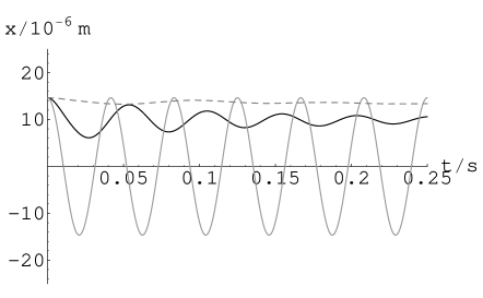
Figure 1: Time evolution of the center of mass of the fermion cloud at the lattice height $s=0$ (grey line), $s=3$ (black line), and $s=8$ (dashed line).

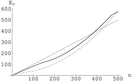
Figure 2: Energy spectrum of a single atom in the combined one-dimensional potential at the lattice height $s=0$ (grey line), $s=3$ (black line), and $s=8$ (dashed line). The energy unit is the energy quantum of the axial harmonic oscillator. The ground state energies are set to zero. A transition from a linear spectrum (harmonic oscillator) to a quadratic one occurs when the lattice is imposed. The quadratic part of the spectrum corresponds to localized states. Non-localized states appear again for higher energies, see the black line which becomes linear for $n>450$.

In the absence of the lattice potential ($s=0$) the system is reduced to a harmonic oscillator and the average position oscillates freely showing the characteristic dipole oscillation in a harmonic potential. None of the eigenstates is localized and the corresponding energy spectrum is linear. The energy quantum or the difference between the consecutive eigenvalues gives the frequency of the oscillations.

When the height of the lattice is increased to $s=3$, both localized and non-localized eigenstates play a role. The oscillations of the system are damped, which can be understood as follows. According to the formula (2), the center of mass of the cloud is a sum periodic terms whose frequencies are given by the differences $(\varepsilon_{n}-\varepsilon_{m})/\hbar$ between the eigenvalues $\varepsilon_{n}$ of the dynamical Hamiltonian. When the eigenvalues are not evenly spaced, destructive interference causes dephasing.

Increasing the lattice height also increases the offset of the dipolar oscillations since more and more particles become localized. When the height of the lattice is increased to $s=8$, localized eigenstates dominate. The system is almost frozen to its initial position. The energy spectrum becomes almost quadratic. The spectrum corresponds to states that are localized in individual lattice potential sites. Neighbouring sites are shifted in energy according to the superimposed harmonic potential, therefore the quadratic form of the spectrum (difference in energy of two localized particles depends essentially only on their locations in the lattice). Actually each energy is doubly degenerate (the symmetric and the antisymmetric states formed of lattice sites at opposite sides of the center) which can be resolved by a closer look at the spectrum. Therefore, to be accurate, localized particles correspond to a superpositions of these doubly degenerate states. Representative examples of localized and non-localized eigenstates are shown in Figure 3.

It is noteworthy that in the intermediary region lowest-lying states are not localized. This is indicated by the linear parts in the spectra near origin. Hence the atoms do not tend to localize when the system is cooled down to ultra-low temperatures, on the contrary. Note that also higher energy states may be unlocalized, i.e. have a linear spectrum, as is shown for one set of parameter values in Figure 2. This is associated with the existence of higher bands of the optical lattice potential. Such states may affect the localization and oscillation behaviour of the gas significantly in higher temperatures.

Figure 3: The two eigenstates (a) and (c) of the lowest energy associated to the potential (e) with parameters $k=3$ and $A=10$ form a quasidegenerate pair. In a superposition of such states, the particle is localized in one of the wells of the potential (e). Relating to Figure 2, such states correspond to a doubly degenerate pair of eigenvalues in a quadratic spectrum. The eigenstates (b) and (d) associated to the potential (f) with parameters $k=12$ and $A=30$ are not localized. They resemble the eigenstates of the harmonic oscillator, modulated by the lattice potential. They correspond to a linear spectrum and their energies are not degenerate.

The results are in very good qualitative and quantitative agreement both with the experiment and the semiclassical approximation presented in [5]. We compared our simulations also to two earlier experiments [3, 4] by Modugno et al. In these cases the experimentalists observed oscillations with considerably larger amplitude and higher frequency than what was predicted by the simulations. We believe that this was simply because the physical parameters used in these experiments were much more demanding for our numerical method and would have required more eigenstates to be calculated than was currently possible. The larger the displacement and the particle number, and the higher the temperature, the more eigenstates are needed for reliable results. The computer resources at our disposal were rather modest so that we have hardly pushed the method to its limits.

5 Conclusions

We have analyzed the energy spectrum and motion of a Fermi gas in a combined potential. The harmonic potential alone has a linear spectrum and shows dipole oscillations of the gas when the trap center is displaced. Introducing the periodic potential transforms the spectrum gradually into quadratic one and the gas becomes localized. Intermediate cases show damped oscillations around the displaced center position. Our approach is complementary to the semiclassical analysis presented in [5, 9], and is in good qualitative agreement with the experiments. For the parameter values which are not too challenging from the numerical point of view the results agree also quantitatively with both the experiments and the semiclassical analysis.

It is important to note that the quantum transport in the combined harmonic and periodic potential is qualitatively rather different from the Bloch oscillation or Wannier-Stark ladder behaviour in tilted periodic potentials. The two cases approach each other only when the gas moves in a region where the harmonic trap can be approximated by a linear potential. This requires a much shallower trap than that used in the experiments [3, 4, 5]. Understanding the behaviour of the non-interacting Fermi gas sets the basis for investigating effects of interactions [4, 10] and eventually superfluidity [11, 12].

Appendix

In this appendix we formulate the reduction from many-particle to single-particle state in the language of symplectic geometry. This formulation may be helpful in using the reduction in a more systematic way and perhaps for more general purposes.

Let us first recall some concepts of classical mechanics using a point-like particle moving in three-dimensional space as an example. The configuration space of the particle is just $C=\mathbb{R}^{3}$ whereas the coordinates of phase space $M\simeq\mathbb{R}^{3}\times\mathbb{R}^{3}$ include the momentum $\mathbf{p}$ as well as the position $\mathbf{x}$. In mathematical terms, the phase space is the cotangent space $T^{*}C$ of the configuration space and it comes equipped with a canonical non-degenerate two-form

$$\omega=\sum_{k=1}^{3}dp^{k}\wedge dx^{k},$$

which is known as the symplectic form while the pair $(M,\omega)$ is referred to as a symplectic manifold. The symmetries of the phase space are the diffeomorphisms of $M$ preserving $\omega$. Accordingly, infinitesimal symmetries are the vector fields $A$ on $M$ whose Lie derivative satisfy $L_{A}\omega=0$. Then each infinitesimal symmetry generates a one-parameter group of symmetries at least locally, where the correspondence is given by the flow of the vector field.

Under some mild conditions we can associate a classical observable or a function $H_{A}$ on the phase space $M$ to an infinitesimal symmetry $A$. The observable is defined by the equation

$$\omega(A,B)=dH_{A}(B)$$

which is required to be valid for all vector fields $B$ on $M$. In particular, since the time-evolution of a classical mechanical system preserves the symplectic form, it is generated by an observable, which is know as the Hamiltonian. In the example above it is clear that both translations and rotations are symmetries of the phase space. An infinitesimal translation is just a three-vector $\mathbf{t}\in\mathbb{R}^{3}$, and the corresponding observable is

$$H_{\mathbf{t}}(\mathbf{x},\mathbf{p})=\mathbf{p}\cdot\mathbf{t}.$$

Similarly, an infinitesimal rotation can be given by a three-vector $\mathbf{r}$ as $\mathbf{r}\cdot\mathbf{R}$ where the components of $\mathbf{R}$ are the infinitesimal rotations about the coordinate axes. The associated classical observable is then

$$H_{\mathbf{r}}(\mathbf{x},\mathbf{p})=(\mathbf{x}\times\mathbf{p})\cdot\mathbf{r}.$$

The general pattern emerging is that given a Lie algebra $\mathfrak{g}$ of infinitesimal symmetries, the collection of associated observables is most conveniently expressed as a map $\rho$ from the phase space $M$ to the dual $\mathfrak{g}^{*}$, that is, the space of linear maps $\mathfrak{g}\to\mathbb{R}$. In this way we associated the momentum $\mathbf{p}$ to the translations and the impulse moment $\mathbf{x}\times\mathbf{p}$ to the rotations. Therefore the map $\rho:M\to\mathfrak{g}^{*}$ defined by the equation

$$(\rho(x),A)=H_{A}(x)$$

for all $A\in\mathfrak{g}$ and $x\in M$ is known as the moment map. The Lie group $G$ corresponding to the Lie algebra $\mathfrak{g}$ acts naturally on both $\mathfrak{g}$ and $\mathfrak{g}^{*}$, and the moment map is equivariant in the sense that $\rho(gx)=g\rho(x)$for all $g$ in $G$.

Returning to quantum mechanics, let $\mathcal{H}$ be a Hilbert space, on which a compact group $G$ acts unitarily. This is the general framework for a quantum mechanical system with the symmetry group $G$. Now the projective space

$$\mathbb{P}(\mathcal{H})=\{v\in\mathcal{H}\>|\>\|v\|=1\}\>/\>U(1)$$

of pure states is canonically a symplectic manifold, on which $G$ acts preserving the symplectic form. Hence from the point of view of symplectic geometry, all that we have said previously applies.

Let $\mathfrak{g}$ be the Lie algebra of $G$. The observable associated to an infinitesimal symmetry $A\in\mathfrak{g}$ is calculated to be the expectation value $H_{A}(v)=\langle v|\hat{A}|v\rangle$ where $\hat{A}$ stands for the representation of $A$ in $\mathcal{H}$. There is also the moment map

$$\rho:\mathbb{P}(\mathcal{H})\to\mathfrak{g}^{*}$$

from the projective space to the dual of $\mathfrak{g}$ defined by the equation

$$H_{A}(v)=(\rho(v),A).$$

Hence the expectation value of $\hat{A}$ in the vector state $v$ is given by $\langle\hat{A}\rangle=(\rho(v),A)$. We can extend the moment map to any state $\Phi$ by linearity. Then the moment map image $\rho(\Phi)$ is a kind of reduced state which can be used to calculate expectation values for all observables in $\mathfrak{g}$. The point is that $\rho(\Phi)$ may be a much simpler object than the state $\Phi$ we started with. Furthermore, the equivariance of the moment map means that

$$\rho(\hat{U}\Phi\hat{U}^{-1})=U\rho(\Phi)U^{-1}$$

for every element $U$ of $G$. In particular, if the Hamiltonian $H$ itself belongs to $\mathfrak{g}$, then the time evolution of the reduced state $\rho(\Phi)$ is given by the usual Schrödinger equation.

In the application we have in mind $G$ is the group of unitary transformations of the single-particle Hilbert space $\mathcal{V}$ and $\mathfrak{g}$ may be identified with the single-particle observables or the Hermitian operators on $\mathcal{V}$. Using the pairing $(B,A)=\Tr(BA)$ we may identify $\mathfrak{g}$ with its dual. Let $\mathcal{H}$ be the fermionic Fock space associated to $\mathcal{V}$. Then $G$ acts naturally on $\mathcal{H}$ and by the general theory

$$\langle\hat{A}\rangle=\Tr(\Phi\hat{A})=\Tr(\rho(\Phi)A)$$ (5)

for any many-particle state $\Phi$ and single-particle observable $A$. It is easy to check that $\rho(\Phi)$ is a positive operator with trace

$$\Tr{\rho(\Phi)}=\Tr(\rho(\Phi)I)=\Tr(\Phi\hat{I})=\Tr(\Phi N)=\langle N\rangle$$

since the number operator $N$ is indeed the representation of $I\in\mathfrak{g}$ in the fermionic Fock space.

In conclusion, we can represent any many-particle state $\Phi$ by a single-particle state $\rho(\Phi)$ when calculating expectation values of single-particle observables. It is easy to calculate $\rho(\Phi)$ explicitly in a given basis $(v_{n})$ of $\mathcal{V}$ using equation 5. In terms of the annihilation and creation operators associated to this basis, the matrix elements of $\rho(\Phi)$ are

$$\rho(\Phi)_{nm}=\Tr(\Phi a_{m}^{\dagger}a_{n})=\langle a_{m}^{\dagger}a_{n}\rangle.$$

Applying the above procedure to the grand canonical ensemble (1) yields

$$\rho(\Phi(0))_{nm}=\frac{e^{\beta(\mu-\epsilon_{n})}\prod_{n\neq k=1}^{\infty}e^{\beta(\mu-\epsilon_{k})}}{\prod_{k=1}^{\infty}e^{\beta(\mu-\epsilon_{k})}}\delta_{nm}=f(\epsilon_{n}-\mu)\delta_{nm},$$

where

$$f(x)=\frac{1}{1+e^{\beta x}}$$

is the Fermi-Dirac distribution which is usually derived using the partition function approach. The preceeding discussion was not just for the sake of an appealing generalization but also to show that the reduction to the single-particle state formalism gives not only the energy distribution but a state matrix obeying the Schrödinger equation.

References

References

- [1] Cataliotti F S, Burger S, Fort C, Maddaloni P, Minardi F, Trombettoni A, Smerzi A and Inguscio M 2001 Science 293 843 Denschlag J H, Simsarian J E, Häffner H, McKenzie C, Browaeys A, Cho D, Helmerson K, Rolston S L and Phillips W D 2002 J. Phys. B: At. Mol. Opt. Phys.35 3095 Liu W M, Fan W B, Zheng W M, Liang J Q and Chui S T 2002 Phys. Rev. Lett.88 170408 Glück M, Keck F, Kolovsky A R and Korsch H J 2001 Phys. Rev. Lett.86 3116 Greiner M, Mandel O, Esslinger T, Hänsch T W and Bloch I Nature 415 39 Anderson B P and Kasevich M A 1998 Science 282 1686
- [2] Dahan M B, Peik E, Reichel J, Castin Y and Salomon C 1996 Phys. Rev. Lett.76 4508 Wilkinson S R, Bharucha C F, Madison K W, Qian Niu and Raizen M G 1996 Phys. Rev. Lett.76 4512 Morsch O, Müller J H, Cristiani M, Ciampini D and Arimondo E Phys. Rev. Lett.87 140402
- [3] Modugno G, Ferlaino F, Heidemann R, Roati G and Inguscio M 2003 Phys. Rev. A 68 011601 (R)
- [4] Ott H, de Mirandes E, Ferlaino F, Roati G, Modugno G and Inguscio M 2004 Phys. Rev. Lett.92 160601
- [5] Pezze L, Pitaevskii L P, Smerzi A, Stringari S, Modugno G, de Mirandes E, Ferlaino F, Ott H, Roati G and Inguscio M 2004 Preprint cond-mat/0401643
- [6] Roati G, de Mirandes E, Ferlaino F, Ott H, Modugno G and Inguscio M 2004 Preprint cond-mat/0402328
- [7] Rigol M and Muramatsu A 2003 Preprint cond-mat/0311444
- [8] Hooley C and Quintanilla J 2003 Preprint cond-mat/0312079
- [9] Kennedy T A B 2004 Preprint cond-mat/0402166
- [10] Orso G, Pitaevskii L P and Stringari S 2004 Preprint cond-mat/0402532
- [11] Rodrígues M and Törmä P 2004 Phys. Rev. A 69 041602 (R)
- [12] Wouters M, Tempere J and Devreese J T 2003 Preprint cond-mat/0312154