Effect of the shot-noise on a Coulomb blockaded single Josephson junction

Abstract

We have investigated how the Coulomb blockade of a mesoscopic Josephson junction in a high-impedance environment is suppressed by shot noise from an adjacent junction. The presented theoretical analysis is an extension of the phase correlation theory for the case of a non-Gaussian noise. Asymmetry of the non-Gaussian noise should result in the shift of the conductance minimum from zero voltage and the ratchet effect (nonzero current at zero voltage), which have been experimentally observed. The analysis demonstrates that a Coulomb blockaded tunnel junction in a high impedance environment can be used as an effective noise detector.

The Coulomb blockade is very sensitive to fluctuations in an environment. The Johnson-Nyquist noise results in a power-law-like increase of conductance as a function of temperature Aver ; SZ ; IN : $G\propto T^{2\rho-2}$. The exponent of the power law, $2\rho-2$, is governed by the parameter $\rho=R/R_{Q}$ where the resistance $R$ describes the dissipative ohmic environment and $R_{Q}=h/4e^{2}$ is the quantum resistance. Tuning the dissipative parameter $\rho$ one expects the quantum or dissipative transition (superconductor–insulator transition) at $\rho=1$, which was revealed experimentally Penttila . Then in the case of large exponents $2\rho-2\gg 1$ (the insulator state), there is a high resolution against tiny changes in temperature, or alternatively, a high sensitivity to thermal noise.

One would expect that the Coulomb blockaded tunnel junction would be sensitive to other noise sources as well. In Ref. SN, the Coulomb blockade of Cooper pairs was used to detect shot noise induced by a separately biased superconductor-insulator-normal metal (SIN) tunnel junction. The current through SIN was found to strongly reduce the Coulomb blockade of Cooper pairs. This has shown a way to use a Josephson tunnel junction for “noise spectroscopy”, and other modifications of this method of noise investigation have been discussed in the literature SNO . However, the theoretical analysis given in Ref. SN, was far from complete: (i) While the experiment was done in the insulator state $\rho\gg 1$, the theoretical analysis was performed for $\rho<1$ using the perturbation theory with respect to shot noise.(ii) The theory could not explain the asymmetry of observed $IV$ curves (shift of the conductance minimum from zero voltage).

The present Letter suggests a theory for the effect of shot noise from an independent source on a Coulomb blockaded Josephson junction. The junction is in the insulator state with high impedance environment $\rho\gg 1$, which is most suitable for purposes of noise detection. The theory shows that since shot noise is non-Gaussian and asymmetric Les , the $IV$ curves should also be asymmetric, i.e., conductance is not an even function of voltage. This should result in the shift of the conductance minimum and the ratchet effect (a finite current at zero voltage bias on the junction BG ), which have already been observed experimentally exp . Asymmetry of $IV$ curves originates from odd moments of the shot noise, which are now intensively discussed theoretically Odd , but are quite difficult to detect experimentally by other methods OddE . This is a manifestation of rich possibilities of noise detection with Coulomb blockaded junctions. The present theory addresses shot noise in a Josephson junction, but apparently it can be generalized to other types of noise and to a Coulomb blockaded normal junction. So the latter can be used for noise detection as well.

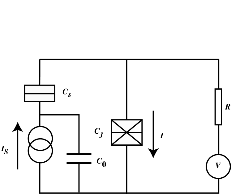
Figure 1: Electric circuit.

The electric circuit for our analysis is shown in Fig. 1. The Josephson tunnel junction with capacitance $C_{J}$ is voltage-biased via the shunt resistor $R$. Parallel to the Josephson junction there is another junction (noise junction) with the capacitance $C_{s}$ connected with an independent DC current source. The role of very large capacitance $C_{0}$ is to shortcircuit the large ohmic resistance of the current source for finite frequencies. The current $I_{S}$ through the noise junction produces shot noise, which affects the $IV$ curve of the Josephson junction. Let us recall well known results concerning the $IV$ curve without shot noise ($I_{S}=0$). We assume that the Josephson coupling energy $E_{J}\cos\varphi$ ($\varphi$ is the Cooper-pair phase across the Josephson junction) is weak in comparison with the Coulomb energy $E_{C}=e^{2}/2C$, where $C=C_{s}+C_{J}$, and the former can be considered as a perturbation. Then the Golden Rule gives for the current of Cooper pairs Aver ; IN :

$$I={\pi eE_{J}^{2}\over\hbar}[P(2eV)-P(-2eV)]~{},$$ (1)

where the function

$$P(E)={1\over 2\pi\hbar}\int_{-\infty}^{\infty}dt\,e^{iEt}\left\langle e^{i\varphi(t_{0})}e^{-i\varphi(t_{0}-t)}\right\rangle~{}$$ (2)

characterizes the probability to excite an environment mode with the energy $E$. Since we use the perturbation theory with respect to $E_{J}$ we can calculate phase fluctuations neglecting $E_{J}$, i.e., treating the Josephson junction as a capacitor. The crucial assumption in the phase-fluctuation theory (or $P(E)$ theory) is that the phase fluctuations are Gaussian IN and

$$\langle e^{i\varphi(t_{0})}e^{-i\varphi(t_{0}-t)}\rangle\approx e^{J_{0}(t)}~{},$$ (3)

where the phase–phase correlator

$$J_{0}(t)=\langle[\varphi(t)-\varphi(0)]\varphi(0)\rangle=J_{R}(t)+iJ_{I}(t)$$

$$=2\int_{-\infty}^{\infty}{d\omega\over\omega}\frac{\mbox{Re}Z(\omega)}{R_{Q}}\frac{e^{-i\omega t}-1}{1-e^{-\beta\hbar\omega}}$$ (4)

is a complex function of time determined by the Johnson-Nyquist noise in the environment, i.e., in the electric circuit with the impedance $Z(\omega)$. Here $\beta=1/k_{B}T$ is the inverse temperature. Then the current is

$$I=-{2eE_{J}^{2}\over\hbar^{2}}\mbox{Im}\int_{0}^{\infty}dte^{J_{0}(t)}\sin\left(2eVt\over\hbar\right)$$ (5)

and the zero-bias conductance is given by

$$G_{0}=\left.{dI\over dV}\right|_{V\rightarrow 0}=-{4e^{2}E_{J}^{2}\over\hbar^{3}}\mbox{Im}\int_{0}^{\infty}t\,dte^{J_{0}(t)}\,.$$ (6)

In our case $Z(\omega)=(1/R+i\omega C)^{-1}$, and at $T\to 0$ ($t>0$):

$$J_{0}(t)=\rho\left[-e^{t/\tau}\mbox{E}_{1}\left({t\over\tau}\right)-e^{-t/\tau}\mbox{E}_{1}\left(-{t\over\tau}+i0\right)\right.$$

$$\left.-2\ln{t\over\tau}-2\gamma-i\pi\right]\approx\rho\left[{t^{2}\over\tau^{2}}\left(\ln{t\over\tau}+\gamma-{3\over 2}\right)-{i\pi t\over\tau}\right]\,,$$ (7)

where $\tau=RC$, $\gamma=0.577$ is the Euler constant, and $\mbox{E}_{1}(z)=\int_{1}^{\infty}(e^{-zt}/t)\,dt$ is the exponential integral AS . The second expression yields the short-time expansion ($t\ll\tau$). The small imaginary correction $+i0$ to the argument of one of the exponential integrals is important for analytic continuation of $\mbox{E}_{1}(z)$ from real $t$ to the complex plane AS . At long times $t\gg\hbar\beta\gg\tau$ one cannot ignore the temperature, which determines the phase diffusion: $J_{R}(t)\approx-2\pi\rho t/\hbar\beta=-2\pi\rho k_{B}Tt/\hbar$. In the insulator state $\rho>1$ in the zero-temperature limit the conductance $G(T)\propto T^{2(\rho-1)}$ vanishes, and the current depends nonanalytically on voltage: $I\propto V^{2\rho-1}$.

One can take into account shot noise simply by adding the shot noise contribution to the correlator $J_{0}(t)$. Then the fluctuating phase $\varphi=\varphi_{0}+\varphi_{s}$ consists of two terms: $\varphi_{0}$ from Johnson-Nyquist noise, and $\varphi_{s}$ from shot noise. Since the fluctuations are uncorrelated the phase–phase correlator is a superposition of two noise contributions: $J(t)=J_{0}(t)+J_{s}(t)$. At long times $t\gg\tau$ the shot noise modifies the phase diffusion: $J_{0}(t)+J_{s}(t)=-2\pi\rho k_{B}(T+T_{N})t/\hbar$, where $T_{N}=e|I_{S}|R/2k_{B}$ is the noise temperature. As a result, the conductance power-law expression changes: $G\sim(T+T_{N})^{2\rho-2}$. At $T=0$ this yields a nonanalytic power-law dependence on the noise current: $G\propto|I_{S}|^{2\rho-2}$. But this approach used in Ref. SN fails at $\rho\gg 1$, which is the most interesting case for noise detection. It ignores the odd moments of shot noise, since the correlator $J_{s}(t)=\langle[\varphi_{s}(t)-\varphi_{s}(0)]\varphi_{s}(0)\rangle$ is quadratic with respect to $\varphi_{s}$.

In the theory for the case $\rho\gg 1$ one should abandon Eq. (3), which assumes that the noise is Gaussian. On the other hand, we assume that the fluctuation $\varphi_{s}$ is classical and the values of $\varphi_{s}$ at different moments of time commute. Since the equilibrium noise and the shot noise are uncorrelated, the generalization of Eq. (5) is

$$I=-{2eE_{J}^{2}\over\hbar^{2}}\mbox{Im}\left\{\int_{0}^{\infty}dte^{J_{0}(t)}\left\langle\sin\left({2eVt\over\hbar}+\Delta\varphi_{s}\right)\right\rangle\right\}.$$ (8)

Here $\Delta\varphi_{s}=\varphi_{s}(t_{0})-\varphi_{s}(t_{0}-t)$. Subtracting from (8) the current at $\Delta\varphi_{s}=0$ given by Eq. (5) we receive the shot-noise contribution to the current (the only contribution at $T\to 0$):

$$\Delta_{s}I=-{2eE_{J}^{2}\over\hbar^{2}}\mbox{Im}\left\{\int_{0}^{\infty}dte^{J_{0}(t)}\left[\cos{2eVt\over\hbar}\left\langle\sin\Delta\varphi_{s}\right\rangle\right.\right.$$

$$\left.\left.+\sin{2eVt\over\hbar}(\left\langle\cos\Delta\varphi_{s}\right\rangle-1)\right]\right\}\,.$$ (9)

Now we want to calculate the shot-noise fluctuations $\varphi_{s}$. The charge transport through the noise junction is a sequence of current peaks $\delta I=\mbox{sign}(I_{S})e\sum_{i}\delta(t-t_{i})$, where $t_{i}$ are the random moments of time when an electron crosses the junction Blanter . We neglect the duration of the tunneling event itself. The positive sign of $I_{S}$ corresponds to the current shown in Fig. 1. Any peak generates a voltage pulse at the Josephson junction: $V_{s}(t)=\mbox{sign}(I_{S})(e/C)\sum_{i}\Theta(t-t_{i})e^{-(t-t_{i})/\tau}$ where $\Theta(t)$ is the step function. After using the Josephson relation $\hbar\partial\varphi/\partial t=2eV$ one finds that $\varphi_{s}$ is given by a sequence of phase jumps at the Josephson junction:

$$\varphi_{s}(t)=\mbox{sign}(I_{S}){2e^{2}\tau\over\hbar C}\sum_{i}\Theta(t-t_{i})\left[1-e^{-(t-t_{i})/\tau}\right]$$

$$=\mbox{sign}(I_{S})\pi\rho\sum_{i}\Theta(t-t_{i})\left[1-e^{-(t-t_{i})/\tau}\right]~{}.$$ (10)

The phase difference between two moments $t_{0}$ and $t_{0}-t$ can be presented as $\Delta\varphi_{s}=\sum_{i}\delta\varphi_{s}(t,t_{0}-t_{i})$, where

$$\delta\varphi_{s}(t,\tilde{t})=\mbox{sign}(I_{S})\pi\rho\left\{\Theta(\tilde{t})\left[1-e^{-(\tilde{t})/\tau}\right]\right.$$

$$\left.-\Theta(\tilde{t}-t)\left[1-e^{-(\tilde{t}-t)/\tau}\right]\right\}~{}.$$ (11)

is the phase difference generated by a single current peak and $\tilde{t}=t_{0}-t_{i}$. Since phase jumps are not small for $\rho\gg 1$, one cannot expand the sine and cosine functions in Eq. (9).

For small currents $|I_{S}|\ll e/\tau$ through the noise junction the voltage pulses and phase jumps are well separated in time. Then the average powers of the phase difference can be approximately estimated as

$$\left\langle\Delta\varphi_{s}^{n}\right\rangle=\sum_{i}\left\langle[\delta\varphi_{s}(t,t_{0}-t_{i})]^{n}\right\rangle$$

$$={|I_{S}|\over e}\int_{-\infty}^{\infty}d\tilde{t}[\delta\varphi_{s}(t,\tilde{t})]^{n}~{}.$$ (12)

The averaging is performed over the random sequences of moments $t_{i}$, which eliminates any dependence on the time $t_{0}$. In Eq. (12) we neglected cross-terms, which contain the phases from more than one pulse and are proportional to higher powers of a small parameter $|I_{S}|\tau/e$.

Equation (12) can be extended on any function of $\Delta\varphi_{s}$, which vanishes at $\Delta\varphi_{s}\rightarrow 0$, and hence we obtain

$$\langle\sin\Delta\varphi_{s}\rangle={|I_{S}|\over e}\int_{-\infty}^{\infty}d\tilde{t}\sin\delta\varphi_{s}(t,\tilde{t})$$

$$={I_{S}\tau\over e}\left\{{\pi\over 2}+\mbox{si}\left[r\left(1-e^{-t/\tau}\right)\right]\right.$$

$$\left.+\sin r\left[\mbox{ci}r-\mbox{ci}\left(re^{-t/\tau}\right)\right]-\cos r\left[\mbox{si}r-\mbox{si}\left(re^{-t/\tau}\right)\right]\right\},$$ (13)

$$\langle\cos\Delta\varphi_{s}\rangle-1={|I_{S}|\over e}\int_{-\infty}^{\infty}d\tilde{t}\left[\cos\delta\varphi_{s}(t,\tilde{t})-1\right]$$

$$={|I_{S}|\tau\over e}\left\{-{t\over\tau}+\cos r\left[\mbox{ci}r-\mbox{ci}\left(re^{-t/\tau}\right)\right]\right.$$

$$\left.+\sin r\left[\mbox{si}r-\mbox{si}\left(re^{-t/\tau}\right)\right]+\mbox{ci}\left[r\left(1-e^{-t/\tau}\right)\right]\right.$$

$$\left.-\gamma-\ln\left[r\left(1-e^{-t/\tau}\right)\right]\right\}~{},$$ (14)

where $\mbox{si}(x)=-\int_{x}^{\infty}\sin t\,dt/t$ and $\mbox{ci}(x)=-\int_{x}^{\infty}\cos t\,dt/t$ are sine and cosine integral functions, and $r=\pi\rho$.

Analyzing the $IV$ curve at small voltage bias, one can expand Eq. (9 ) in $V$:

$$\Delta_{s}I=I_{0}+G_{s}V+aV^{2}+bV^{3}~{},$$ (15)

where

$$G_{s}=-{4e^{2}E_{J}^{2}\over\hbar^{3}}\mbox{Im}\int_{0}^{\infty}t\,dte^{J_{0}(t)}[\left\langle\cos\Delta\varphi_{s}\right\rangle-1]$$ (16)

is the shot-noise conductance, the constant current

$$I_{0}=-{2eE_{J}^{2}\over\hbar^{2}}\mbox{Im}\int_{0}^{\infty}dte^{J_{0}(t)}\left\langle\sin\Delta\varphi_{s}\right\rangle$$ (17)

determines the ratchet effect, and the constants

$$a={4e^{3}E_{J}^{2}\over\hbar^{4}}\mbox{Im}\int_{0}^{\infty}t^{2}\,dte^{J_{0}(t)}\left\langle\sin\Delta\varphi_{s}\right\rangle$$ (18)

and

$$b={8e^{4}E_{J}^{2}\over 3\hbar^{5}}\mbox{Im}\int_{0}^{\infty}t^{3}\,dte^{J_{0}(t)}[\left\langle\cos\Delta\varphi_{s}\right\rangle-1]$$ (19)

determine the curvature of the conductance-voltage plot and the shift of the conductance minimum.

In the high-impedance limit $\rho\gg 1$ it is possible to calculate the parameters of the $IV$ curve analytically. As one can see below, the most important contribution to the integrals comes from $t\sim\tau/\sqrt{r}$. Since $r=\pi\rho$ is large, these values of $t$ are small compared to $\tau$ and one can use the small-argument expansion for the Johnson-Nyquist correlator given in Eq. (7). On the other hand the arguments $rt/\tau\sim\sqrt{r}$ of the sine and the cosine integrals are large and one should use asymptotic expansions for them: $\mbox{si}(x)\sim-\cos x/x$, $\mbox{ci}(x)\sim\sin x/x$. Let us consider, for example, the integral for $G_{s}$:

$$G_{s}\approx-{4eE_{J}^{2}\tau\over\hbar^{3}}|I_{S}|\int_{0}^{\infty}t\,dt\mbox{Im}\left\{e^{J_{0}(t)}\right\}{\sin\left[r\left(1-e^{-t/\tau}\right)\right]\over r\left(1-e^{-t/\tau}\right)}$$

$$\approx{4eE_{J}^{2}\tau^{2}\over\hbar^{3}r}|I_{S}|\int_{0}^{\infty}dt\exp\left(-\rho{t^{2}\over\tau^{2}}\ln{\tau\over t}\right)\sin^{2}{rt\over\tau}$$

$$\approx{\sqrt{2}\pi eE_{J}^{2}\tau^{3}\over\hbar^{3}r^{3/2}\sqrt{\ln r}}|I_{S}|\approx{\pi^{5/2}E_{J}^{2}C^{3}\over 4e^{5}\sqrt{2\ln\rho}}\rho^{3/2}|I_{S}|~{}.$$ (20)

In a similar way one can calculate the integrals determining the other parameters of the IV-curve:

$$I_{0}={\pi^{2}E_{J}^{2}C^{2}\over 8e^{4}}\rho I_{S},~{}a={I_{S}\over|I_{S}|}{C\over 2e}G_{s},~{}b=-{\pi^{2}C^{2}\rho\over 6e^{2}\ln\rho}G_{s}.$$ (21)

If the current $I_{S}$ through the second (noise) junction is not small compared to $e/\tau$ the voltage (phase) pulses start to overlap. Eventually at further growth of the current, so that $|I_{S}|\gg e/\tau$, the current fluctuations around the average value become very small. In this limit with a good accuracy the phase shift $\Delta\varphi_{s}(t)$ is a linear function of time, proportional to the voltage drop $I_{S}R$ on the shunt resistance, and the voltage at the Josephson junction is $V+I_{S}R$. Then as a function of the voltage bias $V$ the $IV$ curve would be asymmetric. In particular, the conductance would have a minimum at $V_{min}=-I_{S}R$, and not at $V=0$. However, for small $I_{S}$ when the electron transport through the noise junction is a sequence of well separated current pulses the asymmetry parameters are essentially different from the electric-circuit effects at large currents, even though they have the same signs.

The ratchet effect can be quantified by the ratio of currents (the current gain) at zero voltage bias: $\beta_{0}=I_{0}/I_{S}$. Our analysis is valid until $\beta_{0}<1$. If $\beta_{0}\gg 1$, a single current pulse at the noise junction is able to produce many Cooper pair tunnelings through the Josephson junction. But then the shot noise at the latter junction would be more important than the noise at the former. Moreover, according to Ref. IN, (Sec. 5.2) the condition $\beta_{0}<1$ is required for validity of the perturbation theory used to calculate the current through the Josephson junction.

In contrast to the equilibrium Johnson-Nyquist-noise governed conductance, which is a nonanalytic function of $V$ in the $T=0$ limit determined by long-time correlations Aver ; SZ ; IN , the shot-noise governed conductance for large $\rho$ has a leading analytic contribution, which comes from short times $\sim\tau/\sqrt{\rho}$ as evident from Eq. (20). Without shot noise the analytic contribution exactly vanishes. One can see it by rotating the integration path in Eq. (6) from the real to the negative imaginary axis in the complex plane. After rotation the integral becomes purely real while the conductance is determined by the imaginary part of the integral. For the purely equilibrium noise the approximation used in Eq. (20) is invalid since the integrand is a strongly oscillating function. But even in the presence of shot noise one can use Eq. (20) only until the conductance integral is convergent at long times $t\gg\tau$. In this limit according to Eq. (7 ) the Johnson–Nyquist correlator $J_{0}(t)\propto-2\rho\ln t$ and the shot noise correlator $\left\langle\cos\Delta\varphi_{s}\right\rangle\propto t$ [see Eq. (14)]. Then the integral for the conductance $G_{s}$ is convergent only if $\rho>1.5$. As long as this inequality is satisfied, $G_{s}$ is linear with respect to $|I_{S}|$. But for $\rho<1.5$ the nonanalytic contribution $G\propto|I_{S}|^{2\rho-2}$, which was derived in Ref. SN, , becomes more important. Thus the transition from nonanalytic to analytic behavior of $G_{s}$ should occur at $\rho=1.5$.

We assumed that the current $I_{S}$ was small, but not so small that Johnson-Nyquist noise from the noise junction could compete with the shot noise. This is achieved by a high resistance $R_{s}$ of the noise junction: $R_{s}I_{S}\gg k_{B}T/e~{},~{}\hbar\omega/e$ PH . Here the relevant frequency is $\omega\sim\sqrt{\rho}/\tau$. These conditions are satisfied in the experiment, which is compared with our theory exp .

In summary, we have presented a theory of the effect of shot noise from an independent source on the Coulomb blockaded Josephson junction in a high-impedance environment. Though we used the framework of phase correlation theory, we essentially modified it by admitting that fluctuations are not Gaussian. The analysis takes into account the asymmetry of shot noise characterized by its odd moments. For high impedance environment the effect is so strong that the expansion in moments is not valid and was not used in the analysis. The asymmetry of the shot noise results in asymmetry of the $IV$ curve: the shift of the conductance minimum from the zero bias and the ratchet effect, which have been observed experimentally exp . Altogether, the analysis demonstrates, that the Coulomb blockaded tunnel junction in a high impedance environment can be employed as a sensitive detector of shot noise. We expect that other sources of noise (e.g., $1/f$–noise), produce similar effects.

I acknowledge collaboration with Julien Delahaye, Pertti Hakonen, Tero Heikkilä, Rene Lindell, Mikko Paalanen, and Mikko Sillanpää. Also I appreciate interesting discussions with Dmitry Averin, Marcus Büttiker, Daniel Esteve, Joseph Imry, Yeshua Levinson, Yuval Oreg, Michael Reznikov, Cristian Urbina, Andrei Zaikin, and Alexander Zorin. The work was supported by the Academy of Finland, by the Large Scale Installation Program ULTI-3 of the European Union, and by the grant of the Israel Academy of Sciences and Humanities.

References

- (1) D.V. Averin, Yu.V. Nazarov, and A.A. Odintsov, Physica B 165&166, 945 (1990).
- (2) G. Schön and A.D. Zaikin, Phys. Rep. 198, 237 (1990).
- (3) G.L. Ingold and Yu.V. Nazarov, in Single Charge Tunneling, Coulomb Blockade Phenomena in Nanostructures, ed. by H. Grabert and M. Devoret (Plenum, New York, 1992), pp. 21-107.
- (4) J.S. Penttilä, Ü. Parts, P.J. Hakonen, M.A. Paalanen, and E.B. Sonin, Phys. Rev. Lett. 82, 1004 (1999).
- (5) J. Delahaye, R. Lindell, M.S. Sillanpää, M.A. Paalanen, E.B. Sonin, and P.J. Hakonen, cond-mat/0209076.
- (6) R. Deblock, E. Onac, L. Gurevich, and L.P. Kouwenhoven, Science 301, 203 (2003); J. Tobiska and Yu.V. Nazarov, con-mat/0308310.
- (7) G.B. Lesovik, Pis’ma Zh. Eksp. Teor. Fiz. 60, 806 (1994)[JETP Lett. 60, 820 (1994)].
- (8) For the “classical” Josephson junction (without Coulomb blockade) the ratchet effect from asymmetric noise was discussed by V. Berdichevsky and M. Gitterman, Phys. Rev. E 56, 6340 (1997).
- (9) R. Lindell, J. Delahaye, M.A. Sillanpää, T.T. Heikkilä, E.B. Sonin, and P.J. Hakonen, cond-mat/0403427, (submitted to Phys. Rev. Lett.)
- (10) L.S. Levitov, H. Lee, and G.B. Lesovik, J. Math. Phys. 37, 4845 (1996); L.S. Levitov and M. Reznikov, cond-mat/0111057; C.W.J. Beenakker, M. Kindermann, and Yu.V. Nazarov, Phys. Rev. Lett. 90, 176802 (2003); A. Shelankov and J. Rammer, Europhys. Lett. 63, 485 (2003); D.B. Gutman and Y. Gefen, Phys. Rev. B 68, 035302 (2003).
- (11) B. Reulet, J. Senzier, and D.E. Prober, Phys. Rev. Lett. 91, 196601 (2003).
- (12) M. Abramowitz and I. A. Stegun, Handbook of Mathematical Functions (Dover, New York, 1972).
- (13) Ya.M. Blanter and M. Büttiker, Phys. Rep. 336, 1 (2000).
- (14) V. Pietilä and T.T. Heikkilä (unpublished).