Dynamics and stability of vortex-antivortex fronts in type II superconductors

Abstract

The dynamics of vortices in type II superconductors exhibit a variety of patterns whose origin is poorly understood. This is partly due to the nonlinearity of the vortex mobility which gives rise to singular behavior in the vortex densities. Such singular behavior complicates the application of standard linear stability analysis. In this paper, as a first step towards dealing with these dynamical phenomena, we analyze the dynamical stability of a front between vortices and antivortices. In particular we focus on the question of whether an instability of the vortex front can occur in the absence of a coupling to the temperature. Borrowing ideas developed for singular bacterial growth fronts, we perform an explicit linear stability analysis which shows that, for sufficiently large front velocities and in the absence of coupling to the temperature, such vortex fronts are stable even in the presence of in-plane anisotropy. This result differs from previous conclusions drawn on the basis of approximate calculations for stationary fronts. As our method extends to more complicated models, which could include coupling to the temperature or to other fields, it provides the basis for a more systematic stability analysis of nonlinear vortex front dynamics.

I Introduction

I.1 Motivation

The properties of type II superconductors have been studied extensively in past decades. The analysis of patterns in the magnetic flux distribution has generally focused on equilibrium vortex phases. The interplay of pinning and fluctuation effects, especially in the high-$T_{c}$ superconductors, gives rise to a rich variety of phases whose main features are by now rather well understood giannirmp ; gianni . In comparison with equilibrium behavior, however, our understanding of the dynamics of vortices, and the dynamical formation of vortex patterns, is still much less well developed.

Recently, experiments with magneto-optical techniques on flux penetration in thin films have revealed the formation of a wide variety of instabilities. An example is the nucleation of dendrite-like patterns in $Nb$ and $MgB_{2}$ films dendrites ; Shantsev ; Shantsev2 . These complex structures consist of alternating low and high vortex density regions and are found in a certain temperature window. Likewise, flux penetration in the form of droplets separating areas of different densities of vortices has been observed in $NbSe_{2}$ droplets . Patterns with branchlike structures have been found also in high-$T_{c}$ materials, like $YBa_{2}Cu_{3}O_{7-x}$ leiderer . In addition, the scaling of the fluctuations of a (stable) vortex front penetrating a thin sample has been studied surdeanu .

Usually the occurrence of dendrite-like patterns in interfacial growth phenomena can be attributed to a diffusion-driven, long-wavelength instability of a straight front, similar to the Mullins-Sekerka instability Mullins-Sekerka found in crystal growth. In this paper we therefore investigate the stability of a straight front of vortices and antivortices which propagate into a type II superconductor. Furthermore, according to the experimental data Frello ; Indenbom ; Koblischka ; Vlasko , the boundary between vortices and antivortices exhibits many features suggestive of a long-wavelength instability.

The nucleation of dendrites associated with the propagation of a flux front into a virgin sample has been attributed to such an interfacial instability. This results from a thermo-magnetic coupling Mints ; Shantsev ; Shantsev2 ; Aranson where a higher temperature leads to a higher mobility, enhanced flux flow, and hence a larger heat generation. However, the cause of the instability at the boundary between fluxes of opposite sign is still being debated. Shapiro and co-workers Shapiro attribute these patterns to a coupling to the temperature field via the heat generated by the annihilation of vortices with antivortices. On the other hand, Fisher et al. Fisher ; Fisher1 claim that an in-plane anisotropy of the vortex mobility is sufficient to generate an instability.

There are several reasons to carefully reinvestigate the idea of an anisotropy-induced instability of propagating vortex-antivortex fronts. First of all, even though this mechanism was claimed to be relevant for the ”turbulent” behavior at the boundaries of opposite flux regions, the critical anisotropy coefficients found on the basis of an approximation Fisher ; Fisher1 correspond to an anisotropy too high to describe a realistic situation, even when a nonlinear relation between the current and the electric field was considered. anisocoeff1 ; anisocoeff2 ; anisocoeff3 . Secondly, the calculation was effectively done for a symmetric stationary interface, rather than a moving one. Thirdly, the physical picture that has been advanced Fisher for the anisotropy-induced instability is that of a shear-induced Kelvin-Helmholtz instability, familiar from the theory of fluid interfaces kelvin . However, it is not clear how far the analogy with the Kelvin-Helmholtz instability actually extends.

In order to try to settle the mechanism that underlines such phenomena, we investigate here the linear stability of the interface between vortices and antivortices without any approximations in the case where the front of vortices propagates with a finite velocity. We perform an explicit linear stability analysis which shows that, in the presence of an in-plane anisotropy, vortex fronts with sufficiently large speed are stable in the absence of coupling to the temperature. We shall see that the issue of the stability of fronts between vortices and antivortices is surprisingly subtle and rich: while we confirm the finding of Fisher et al. Fisher ; Fisher1 that stationary fronts have an instability to a modulated state, our moving fronts are found to be stable for all anisotropies. Moreover, our calculations indicate that the stability of such fronts depends very sensitively on the distribution of antivortices in the domain into which the front propagates, so it is difficult to draw general conclusions.

Besides the intrinsic motivation to understand this anisotropy issue, there is a second important motivation for this work. Our coarse-grained dynamics of the vortex densities is reminiscent of reaction-diffusion equations with nonlinear diffusion. This makes the coarse-grained vortex dynamics very different from the Gaussian diffusive dynamics of a linear diffusion equation. For example, the fact that vortices penetrate a sample with linear density profiles bean is an immediate consequence of this. More fundamentally, the dynamically relevant fronts in such equations with nonlinear diffusion are usually associated with nonanalytic (singular) behavior of the vortex densities — such singular behavior has been studied in depth for the so-called porous medium equation porous1 ; porous2 ; porous3 , which has a similar nonlinear diffusion. In the case we will study, the front corresponds to a line on one side of which one of the vortex densities is nonzero, while on the other side it vanishes identically. In the regime on which we will concentrate, this vortex density vanishes linearly near the singular line. But for other cases encountered in the literature Fisher1 ; otherexp even more complicated non-linear dynamical equations arise that are reminiscent of reaction-diffusion type models in other physical systems. The case of bacterial growth models benjacob ; Judith illustrates that the non-linearity of the diffusion process can have a dramatic effect on the front stability, so a careful analysis is called for. Nevertheless, in our case nonlinear diffusion by itself does not lead to an instability of the front, unlike in the bacterial growth case Judith or viscous fingering Mullins-Sekerka .

From a broader perspective, we see this work as a first step towards a systematic analysis of moving vortex fronts. The linear stability analysis which we will develop can equally well be applied to dynamical models which include coupling to the temperature or in which the current-voltage characteristic is nonlinear. For this reason, we present the analysis in some detail for the relatively simple case where the vortex velocity is linear with respect to the magnetic field gradient and the current. Even then, as we shall see, the basic uniformly translating front solutions can still have surprisingly complicated behavior. We find that the density of vortices which penetrate the sample vanishes linearly for large enough front velocities, but with a fractional exponent for front velocities below some threshold velocity barenblatt . Since the latter regime appears to be physically less relevant, and since we do not want to overburden the paper with mathematical technicalities, we will focus our analysis on the first regime. As stated before, in this regime we find that an anisotropy in the mobility without coupling to the temperature does not give rise to an instability of the flux fronts.

Our analysis will be aimed at performing the full stability analysis of the fronts in the coupled continuum equations for the vortex densities. Our procedure thus differs from the one of Fisher ; Fisher1 in which a sharp interface limit was used. In many physical systems it is often advantageous to map the equations onto a moving boundary effective interface problem, in which the width of the transition zone for the fields is neglected. One can in principle derive the proper moving boundary approximation from the continuum equations with the aid of singular perturbation theory. The analogous case of the bacterial growth fronts Judith indicates, however, that such a derivation can be quite subtle for nonlinear diffusion problems. Indeed it is not entirely clear whether the assumptions used in the sharp interface limit of Ref. Fisher ; Fisher1 are fully justified. For this reason, we have developed an alternative and more rigorous stability analysis which allows for a systematic study on fronts in vortex dynamics.

I.2 The model

The physical situation that we have in mind refers to a semi-infinite 2D thin film in which there is an initial uniform distribution of vortices due to an external field H applied along the $z$ direction. By reversing and increasing the field, a front of vortices of opposite sign penetrates from the edge of the film. We will refer to the original vortices as antivortices with density $n^{-}$, and to the ones penetrating in after the field reversal as vortices with density $n^{+}$. In the region of coexistence of vortices and antivortices, annihilation takes place. Vortices are driven into the interior of the superconducting sample by a macroscopic supercurrent J along the $y$ direction due to the gradient in the density of the internal magnetic field. Flux lines then tend to move along the direction $x$ transverse to the current under the influence of the Lorentz force on each vortex (see e.g. giannirmp ; gianni )

$${\bf F}^{\pm}=\pm\frac{1}{c}{\bf J}\times{\bf\phi}_{0}\,{\bf e_{z}},$$ (1)

where ${\bf\phi}_{0}$ is the quantum of magnetic flux associated with each Abrikosov vortex. We consider the regime of pure flux flow in which pinning can be neglected, while the viscous damping then gives rise to a finite vortex mobility. We follow a coarse-grained hydrodynamic approach in which the fields vary on a scale much larger than the distance between vortices. Since the magnetic flux penetrates in the form of quantized vortices, the total magnetic field in the interior of the thin film can be expressed in a coarse graining procedure through the difference in the density of vortices and antivortices,

$${\bf B}=(n^{+}-n^{-})\,\phi_{0}\,{\bf e_{z}}.$$ (2)

The dynamical equations for the fields of vortices and antivortices are simply the continuity equations

$$\frac{\partial n^{+}}{\partial t} = -{\bf\nabla}\cdot(n^{+}\,{\bf{v}^{+}})-\frac{n^{+}n^{-}}{\tau},$$

$$\frac{\partial n^{-}}{\partial t} = -{\bf\nabla}\cdot(n^{-}\,{\bf{v}^{-}})-\frac{n^{+}n^{-}}{\tau},$$ (3)

where the second term on the right represents the annihilation between vortices of opposite sign. Note that since vortices annihilate in pairs, the total magnetic field $B_{z}$ is conserved in the annihilation process. The annihilation terms depends on the recombination coefficient $\tau$; a simple kinetic gas theory type estimate shows that $\tau^{-1}$ is of order of $v\xi_{0}$, since the cross section of a vortex is of order $\xi_{0}$, the coherence length Shapiro . The velocity $\bf{v}$ can be determined with the phenomenological formula for the flux flow regime:

$$\eta{\bf{v}}^{\pm}=\pm\,{\bf{J}}\times\frac{\phi_{0}}{c}\,{\bf{e}_{z}},$$ (4)

where the Hall term has been neglected with good approximation for a case of a dirty superconductor gianni . The drag coefficient $\eta$ is given by the Bardeen-Stephen model Bardeen and generally depends on the temperature of the sample. In this paper we neglect this important coupling to the temperature, but we will allow the mobility (the inverse of the drag) to be anisotropic. In passing, we also note that the above linear relation between the current J and the flow velocity ${\bf v}^{\pm}$ is often generalized to a nonlinear dependence Fisher1 . For simplicity, we do not consider this case here, but our method can be extended to such situations.

For a type II superconducting material with a Ginzburg-Landau parameter $\kappa\gg 1/\sqrt{2}$, the magnetization of the sample can be neglected, so that ${\bf B}\approx{\bf H}$. Then, by using the Maxwell equation (in which the term related to the displacement currents has been neglected with good approximation)

$${\bf J}=\frac{c}{4\pi}\,{{\bf\nabla}}\,\times\,{\bf B},$$ (5)

together with (2) and (4), and substituting into (3), we get:

$$\frac{\partial n^{+}}{\partial t} = D\,{\bf\nabla}\cdot(n^{+}\,{\bf\nabla}(n^{+}-n^{-}))-\frac{n^{+}n^{-}}{\tau},$$ (6)

$$\frac{\partial n^{-}}{\partial t} = D\,{\bf\nabla}\cdot(n^{-}\,{\bf\nabla}(n^{-}-n^{+}))-\frac{n^{+}n^{-}}{\tau}.$$ (7)

where the coefficient D is given by ${\displaystyle D=\phi_{0}^{2}/(4\pi\eta)}$. This is the system of non-linear differential equations which governs the dynamics of the vortex-antivortex front. The situation that we will study in our analysis is the following. We consider a front of vortices which propagates into the superconducting thin film from the left edge at $x=-L_{x}$ in the positive $x$ direction. At $x=-L_{x}$, we impose the boundary condition that the density of vortices $n^{+}$ is ramped up linearly in time, $n^{+}(-L_{x},t)=Rt$. This corresponds to the field going up linearly, just as in the Bean critical state bean . We impose also that far right at $x\to\infty$, $n^{+}$ vanishes while $n^{-}$ approaches a constant value $n_{\infty}$. Through a rescaling of time and length variables, the coefficients of the equations (6) and (7) can be set to unity. In particular, it is convenient to rescale the time and length variables according to the following transformation:

$$t \rightarrow \frac{t\,n_{\infty}}{\tau},$$

$$x \rightarrow \frac{x}{l_{0}}=x\sqrt{\frac{4\pi\eta}{\phi_{0}^{2}\tau}},$$

$$n \rightarrow \frac{n}{n_{\infty}}.$$ (8)

We will henceforth analyze the equations (6) and (7) with $D=1$ and $\tau=1$.
As we already mentioned in the introduction, and as we shall see in detail below, the above continuum equations have a mathematical singularity at the point where $n^{+}$ vanishes. Of course, in reality there cannot be such a true singularity and our continuum coarse-grained model breaks down at scales of the order of the London penetration depth. In particular, the derivative of the magnetic field and thus the current $\bf{J}$ are not discontinuous with respect to the space variable, but they decrease exponentially in a distance approximately equal to the penetration depth. Effects like thermal diffusion, the finite core size, and the nonlocal relations which are neglected in the London approximation all play a role there, and the Ginzburg-Landau equation would provide a more appropriate starting point. Clearly, if the dynamical behavior of our continuum model would be very sensitively dependent on the nature of the singularity, then this would be a sign that the physics at this cutoff scale would really strongly affect the dynamically relevant long-wavelength dynamics. In practice, however, this is not the case. First of all, our method to do the linear stability analysis is precisely aimed at making sure that the singularities at the level of the continuum equations does not mix with the behavior or pertubations of the front region. Secondly, as we shall see there are no instabilities on scales of the order of the microscopic cutoff provided by the London penetration depth.

I.3 The Method

In our analysis, we first study a planar front which propagates with a steady velocity v along the x direction. By considering the propagation of the front in the comoving frame, we get a system of ordinary differential equations (ODEs) for the vortex and antivortex density fields. The derivation of the uniformly translating solution is discussed in Section II.1. As we will see, the profile that corresponds to the planar front for the density of vortices is singular. In particular, in the regime on which we will focus, the derivative of the vortex density is discontinuous at the point where the field vanishes, while in the low-velocity regime there are higher order singularities. As a consequence of this nonanalytic behavior, the numerical integration of the equations has to be done with care near the singular point.

In Section III, we perform a linear stability analysis of the planar solution. A proper ansatz consists here of two contributions: a perturbation in the line of the singular front and a perturbation of the density field. As we will see, the presence of an in-plane anisotropy means that the (anti)vortex flow velocity is no longer in the same direction as the driving force acting on the (anti)vortices. Hence, contrary to the isotropic case, we have to consider a component of the velocity perpendicular to the driving force. The viscosity is thus represented by a non-diagonal tensor and depends on the angle between the direction of propagation of the front and the fast growth direction given by the anisotropy. By applying a linear stability analysis we get a system of equations for the fields representing the perturbation. Through a shooting method, and by matching the proper boundary conditions, we are then able to determine a unique dispersion relation for the growth rate of the perturbation. In Section IV we treat the case of a stationary front, with a velocity $v=0$. Contrary to the case of a moving front, no singularity in the profiles of the fields is present and the analysis can be carried out in the standard way.

II The planar front

II.1 The equations and boundary conditions

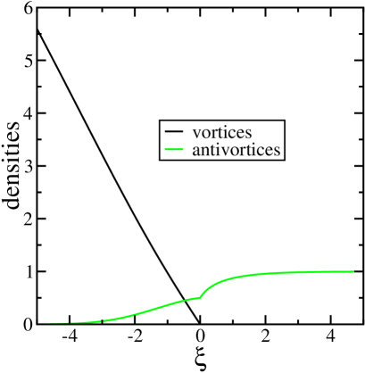
Figure 1: Profile of the planar front for the density of the vortices ($n^{+}$) and antivortices ($n^{-}$) for the case $v=1$.

In this section, we analyze the planar uniformly translating front solutions $n^{+}=n^{+}_{0}(x-vt)$, $n^{-}=n^{-}_{0}(x-vt)$ which are the starting point for the linear stability analysis in the next section. We refer to the system in a comoving frame in which the new coordinate is traveling with the velocity $v$ of the front, ${\displaystyle\xi=x-vt}$. The temporal derivative then transforms into ${\displaystyle\partial_{t}|_{x}=\partial_{t}|_{\xi}-v\partial_{\xi}}$. Since the front is uniformly translating with velocity $v$, the explicit time derivative vanishes. In the comoving frame system, we consider $\xi$ to vary in the spatial interval $[-L,+\infty]$. The equations (6) and (7) become:

$$-v\frac{dn_{0}^{+}}{d\xi} = \frac{d}{d\xi}n_{0}^{+}\,\frac{d}{d\xi}(n_{0}^{+}-n_{0}^{-})-n_{0}^{+}n_{0}^{-},$$ (9)

$$-v\frac{dn_{0}^{-}}{d\xi} = \frac{d}{d\xi}n_{0}^{-}\,\frac{d}{d\xi}(n_{0}^{-}-n_{0}^{+})-n_{0}^{+}n_{0}^{-}.$$ (10)

This is a system of two ODEs of second order. Motivated by the physical problem we wish to analyze, the relevant uniformly translating front solutions obey the following boundary conditions at infinity:

$$\begin{array}[]{ll}\displaystyle\lim_{\xi\rightarrow+\infty}n_{0}^{-}=n_{\infty},&{\displaystyle\lim_{\xi\rightarrow+\infty}\frac{dn_{0}^{-}}{d\xi}=0},\\ \displaystyle\lim_{\xi\rightarrow+\infty}n_{0}^{+}=0,&{\displaystyle\lim_{\xi\rightarrow+\infty}\frac{dn_{0}^{+}}{d\xi}=0}.\end{array}$$ (11)

It is important to note that the constant $n_{\infty}$ can actually be set to unity: by rescaling the density fields as well as space and time, any problem with arbitrary $n_{\infty}$ can be transformed into a rescaled problem with $n_{\infty}=1$. The stability of fronts therefore does not depend on $n_{\infty}$, and in presenting numerical results we always use the freedom to set $n_{\infty}=1$.

On the left, the density of vortices $n^{+}$ increases linearly with time with sweeping rate $R$. After a transient time, because of the annihilation process, the field $n_{0}^{-}$ and its derivative vanish. The dynamical equation (9) for the $n^{+}$ field then yields

$$\frac{dn_{0}^{+}}{d\xi}=-v+\mathcal{O}\left(\frac{1}{n_{0}^{+}}\right),$$ (12)

i.e., we recover the well known critical state result bean that in the absence of antivortices the penetrating $n^{+}$ field varies linearly with slope $-v$. Requiring that this matches the boundary condition $n^{+}(-L_{x},t)=Rt$ for large times at $\xi=-L$ then immediately yields that $R=v^{2}$. It can be easily derived that the density of antivortices decays with a Gaussian behavior on the left. By using indeed the relation (12) for large distances and substituting it in (10), we get:

$$n_{0}^{-}\approx Ae^{-\xi^{2}/4}.$$ (13)

Since the analysis of the planar front profiles and of their stability is naturally done in the comoving $\xi$ frame, we will in practice use a semi-infinite system in the $\xi$ frame, and impose as boundary conditions at $\xi=-L$

$$\begin{array}[]{ll}\displaystyle\lim_{\xi\rightarrow-L}{\displaystyle n_{0}^{-}=0},&\displaystyle\lim_{\xi\rightarrow-L}{\displaystyle\frac{dn_{0}^{-}}{d\xi}=0},\\ \displaystyle\lim_{\xi\rightarrow-L}{\displaystyle n_{0}^{+}=const\gg 1},&\displaystyle\lim_{\xi\rightarrow-L}{\displaystyle\frac{dn_{0}^{+}}{d\xi}}=-v.\end{array}$$ (14)

Of course, in any calculation we have to make sure that $L$ is taken large enough that the profiles $n_{0}^{\pm}$ have converged to their asymptotic shapes.

II.2 Singular behavior of the fronts

Effectively, Eqs. (6-7) and (9-10) have the form of diffusion equations whose diffusion coefficient vanishes linearly in the densities $n^{+}$ and $n^{-}$. As already mentioned before, it is well known, from e.g. the porous medium equation porous1 ; porous2 ; porous3 , that such behavior induces singular behavior at the point where a density field vanishes (see e.g. Ref. Bender ). Because we are looking at fronts moving into the region where $n^{+}=0$, in our case the singularity is at the point where the $n^{+}$ density vanishes. Let us choose this point as the origin $\xi=0$. Then the relevant front solutions have $n^{+}(\xi)=0$ for all $\xi>0$; see Fig. 1 note3 .

Because $n^{-}_{0}(0)\neq 0$, the prefactor of the highest derivative in the $n^{-}$ equation does not vanish at $\xi=0$, and hence one might naively think that $n^{-}$ is nonsingular at this point. However, because of the coupling through the diffusion terms, this is not so. By integrating Eq. (10) over an interval centered around $\xi=0$ and using that the field values $n^{+}_{0}$ and $n^{-}_{0}$ are continuous, one immediately obtains that

$$\lim_{\Delta\xi\rightarrow 0}\left.\left(\frac{dn_{0}^{+}}{d\xi}-\frac{dn_{0}^{-}}{d\xi}\right)\right|_{-\Delta\xi}^{\Delta\xi}=0.$$ (15)

Physically, this constraint expresses the continuity of the derivative of the coarse-grained magnetic field (2). Mathematically, it shows that any singularity in $n^{+}_{0}$ induces precisely the same singularity in $n^{-}_{0}$: to lowest order the two singularities cancel. Fig. 1 illustrates this: one can clearly discern a jump in the derivative of $n^{-}_{0}$ at the point where $n^{+}_{0}$ vanishes with finite slope.

Before we analyze the nature of the singularity in more detail, we note that because of the nonanalytic behavior at $\xi=0$, it is necessary to analyze the region $\xi<0$ where $n^{+}_{0}\neq 0$ separately from the one at $\xi>0$ where $n^{+}_{0}=0$. In the latter regions, the equations simplify enormously, as the remaining terms in Eq. (10) can be integrated immediately. Upon imposing the boundary conditions (11) at infinity, this yields

$$\frac{dn_{0}^{-}}{d\xi}=-v\frac{(n_{0}^{-}-n_{\infty})}{n_{0}^{-}},\hskip 14.22636pt\xi>0.$$ (16)

Let us now analyze of the nature of the singularity at $\xi=0$. As the effective diffusion coefficient of the $n^{+}$-equation is linear in $n^{+}$, analogous situations in the porous medium equation suggest that the field $n^{+}$ vanishes linearly. This motivates us to write for $-1\ll\xi<0$ note4

$$\begin{array}[]{l}{\displaystyle n^{+}_{0}(\xi)=A^{+}_{1}\xi+A^{+}_{2}\xi^{2}+\cdots,}\\ {\displaystyle n^{-}_{0}(\xi)=A^{-}_{1}\xi+A^{-}_{2}\xi^{2}+\cdots+n^{-}_{\rm an}(\xi),}\end{array}$$ (17)

where $n^{-}_{\rm an}(\xi)$ is the analytic function which obeys Eq. (16) for all $\xi$. Clearly, the continuity condition (15) immediately implies

$$A^{+}_{1}=A^{-}_{1}.$$ (18)

If we now substitute the expansion (17) with (18) into Eq. (9) for $n^{+}_{0}$ we get by comparing terms of the same order:

$$\begin{array}[]{l}{\displaystyle{\mathcal{O}}(1):~{}~{}~{}A^{+}_{1}(v-n^{-\prime}_{\rm an})=0,}\\ {\displaystyle{\mathcal{O}}(\xi):~{}~{}~{}4(A^{+}_{2}-A^{-}_{2})-2n^{-\prime\prime}_{\rm an}-n^{-}_{\rm an}=0.}\end{array}$$ (19)

Here $n^{-\prime}_{\rm an}=dn^{-}_{\rm an}/d\xi|_{\xi=0}$, etc. Likewise, if we substitute the expansion into Eq. (10) for $n^{-}_{0}$, we get

$${\displaystyle{\mathcal{O}}(1):~{}~{}~{}2vA^{-}_{1}-2n^{-}_{\rm an}(A^{+}_{2}-A^{-}_{2})=0,}$$ (20)

since the term of order unity involving $n^{-}_{\rm an}$ cancels in view of (16). Higher order terms in the expansion determine the coefficients $A_{2}^{+}$ and $A_{2}^{-}$, and other terms like $A_{3}^{\pm}$ separately, but are not needed here. Together with (16), the above equations (19-20) immediately yield

$$\begin{array}[]{rl}{\displaystyle n_{\rm an}^{-\prime}}=&{\displaystyle v,}\\ {\displaystyle n_{\rm an}^{-}(0)}=&{\displaystyle 1/2},\\ {\displaystyle A^{+}_{1}=A^{-}_{1}}=&{\displaystyle-v+\frac{1}{16v},}\end{array}$$ (21)

where for convenience we have now put $n_{\infty}=1$.

There are two curious features to note about the above result. First of all, $n^{+}_{0}$ always vanishes at the point where $n^{-}_{0}$ is half of the asymptotic value $n_{\infty}$ at infinity. Secondly, note that $A^{+}_{1}$ is negative for $v\geq 1/4$ and positive for $v<1/4$. Since the vortex density $n^{+}$ has to be positive, we see that these uniformly translating front solutions can only be physically relevant for $v\geq 1/4$!

Since the front velocity in this problem is not dynamically selected but imposed by the ramping rate $R=v^{2}$ at the boundary, we do expect physically realistic solutions with $v<1/4$ to exist. In fact, it does turn out that in this regime the nature of the singularity changes: instead of vanishing linearly, $n^{+}_{0}$ vanishes with a $v$-dependent exponent. Indeed, if we write for $-1\ll\xi<0$ note4

$$n^{+}_{0}(\xi) = |\xi|^{\alpha}(A^{+}_{1}+A^{+}_{2}\xi+\cdots),$$ (22)

$$n^{-}_{0}(\xi) = |\xi|^{\alpha}(A^{-}_{1}+A^{-}_{2}\xi+\cdots)+n^{-}_{\rm an}(\xi),$$ (23)

and substitute this into the equations, then, in analogy with the result above, we find

$$\begin{array}[]{rl}{\displaystyle n_{\rm an}^{-\prime}}=&{\displaystyle v,}\\ {\displaystyle n_{\rm an}^{-}(0)}=&{\displaystyle 1/2},\\ {\displaystyle A^{+}_{1}}=&{\displaystyle A^{-}_{1}},\\ {\displaystyle\alpha}=&{\displaystyle\frac{1}{8v^{2}}-1>1},~{}~{}~{}(v<1/4),\end{array}$$ (24)

while again for $\xi>0$ $n^{+}_{0}$ vanishes. A singular behavior with exponent depending on the front velocity $v$ is actually quite surprising for such an equation barenblatt . However, one should keep in mind that this behavior is intimately connected with the initial condition for the $n^{-}$ vortices. If one starts with a case where $n^{-}$ does not approach a constant asymptotic limit on the far right, but instead increases indefinitely, one will obtain solutions where $n^{+}$ vanishes linearly. For this reason, and in order not to overburden the analysis with mathematical technicalities, from here on we will concentrate the analysis on the regime $v\geq 1/4$.

Since our study will limit the stability analysis to fronts with velocity $v\geq 1/4$ in our dimensionless variables, let us check how the scale that we consider relates with the realistic values of flux flow velocities. By considering relations (8) the velocities are measured in units of:

$$v_{0}=\frac{l_{0}n_{\infty}}{\tau} = c\sqrt{\frac{H_{\infty}}{H_{c2}}}\sqrt{\frac{\rho_{n}n_{\infty}v\xi_{0}}{4\pi}},$$ (25)

$$\approx c\sqrt{\frac{\xi_{0}^{2}}{a^{2}}}\sqrt{\frac{\rho_{n}v\xi_{0}}{4\pi a^{2}}},$$

where we have expressed the viscosity $\eta$ in terms of the upper critical field $H_{c2}$ and the normal state resistivity $\rho_{n}$ by using Bardeen . Furthermore, $a$ is the distance between vortices for $\xi\rightarrow\infty$; thus, since $H_{\infty}=\phi_{0}n_{\infty}\approx\phi_{0}/a^{2}$, it follows that $H_{\infty}/H_{c2}\approx\xi_{0}^{2}/a^{2}$. For the constant $\tau$ we have used the estimate $\tau^{-1}=v\xi_{0}$ discussed after Eq. (3). We can then rewrite (25) as

$$v\approx c^{2}\frac{\xi_{0}^{3}}{4\pi a^{4}}\rho_{n}.$$ (26)

By considering typical values in Gaussian units $\rho_{n}\approx~{}10^{-16}s$ for the resistivity of the material, a coherence length $\xi_{0}\approx 2\,10^{-7}$ cm for high-$T_{c}$ compounds and a magnetic field $H_{\infty}\approx 20G$ (which corresponds to a length $a\approx 10^{-4}$ cm), our velocity is then measured in units of $v\approx 1\,cm/s$. This velocity scale is much less than values found typically in the flux flow regime, since in the presence of instabilities fronts of vortices can propagate with much higher velocities of order $10^{4}-10^{6}cm/s$ Shantsev2 . Thus, the regime $v\geq 1/4$ is indeed the physical relevant one.

II.3 Sum and difference variables

At first glance, the equations look like two coupled second order equations. However, there is more underlying structure due to the fact that the annihilation term does not effect the difference $n^{+}-n^{-}$. In order to integrate the set of equations (9-10), it is convenient to consider the following transformations in the variables related to the sum and difference of the density fields:

$$\begin{array}[]{ll}{\displaystyle D}&={\displaystyle n^{+}-n^{-},}\\ {\displaystyle S}&={\displaystyle n^{+}+n^{-}.}\end{array}$$ (27)

In these variables, the equations become

$$-v\frac{dD_{0}}{d\xi} = \frac{d}{d\xi}S_{0}\frac{dD_{0}}{d\xi},$$ (28)

$$-v\frac{dS_{0}}{d\xi} = \frac{d}{d\xi}D_{0}\frac{dD_{0}}{d\xi}-\frac{S_{0}^{2}-D_{0}^{2}}{2}.$$ (29)

By numerically integrating (28-29) and looking for the solutions which satisfy the boundary conditions above, we obtained the uniformly translating front solutions. As Fig. 1 illustrates for $v=1$, the profile is singular at the point where the density of the $n^{+}$ field vanishes linearly, in agreement with the earlier analysis.

Because of this singularity, the numerical integration of the set (28-29) is quite nontrivial. In particular, because of the discontinuity in the derivative of the $n^{+}$ field, the system (28-29) effectively needs to be solved only in the interval $[-L,0[$, as the matching to the behavior for $\xi>0$ has already been translated into the boundary conditions (21). The first equation can be straightforwardly integrated and by combining it with the second, the set reduces to

$$\begin{array}[]{ll}{\displaystyle\frac{dD_{0}}{d\xi}}&={\displaystyle\frac{-v(D_{0}+n_{\infty})}{S_{0}}},\\ {\displaystyle\frac{dS_{0}}{d\xi}}&={\displaystyle\frac{{S_{0}(v(2D_{0}+n_{\infty})){\displaystyle\frac{dD_{0}}{d\xi}}+(S_{0}^{4}-S_{0}^{2}D_{0}^{2})/2}}{{\displaystyle vS_{0}^{2}+(v(D_{0}^{2}+n_{\infty}D_{0}))}}}.\end{array}$$ (30)

One can easily verify that in this formulation, the expression on the right hand side is indefinite at the singular point $\xi=0$, as both the terms in the numerator and denominator vanish. In order to evaluate the expression, it is then necessary to perform an expansion of the numerator and denominator around the critical point values $S=-D=n_{\infty}/2$. From such an analysis one can then recover the relations (21) which we previously obtained from a straightforward expansion of the original equations. Numerically, we integrate the equations by starting slightly away from the singular point with the help of the results from the analytic expansion.

III Front propagation in the presence of anisotropy

III.1 Dynamical equations

As mentioned before, we are interested in the effect that an anisotropy in the vortex mobility could have on the stability of the front. In particular, the motivation for such an investigation is the experimental evidence that an instability for a flux-antiflux front was found in materials with an in-plane $ab$ anisotropy, such as for example $YBa_{2}Cu_{3}O_{7-\delta}$ Koblischka .

In a material characterised by an in-plane anisotropy, the effective viscous drag coefficient depends on the direction of propagation of the front. More precisely, the mobility defined in (4) then becomes a non-diagonal tensor. This leads to a non-zero component of the velocity $v$ perpendicular to the driving Lorentz force. We want to investigate whether the non-collinearity between the velocity and the force is responsible for an instability of the flux-antiflux interface. In the presence of anisotropy, the phenomenological formula (4) then has to be replaced by:

$${\bf{v}}=\hat{\eta}^{-1}{\bf{F}}=\Gamma R^{-1}\left(\begin{array}[]{cc}1&0\\ 0&\alpha\end{array}\right)R{\bf{F}},$$ (31)

where $\Gamma$ is a constant, $\alpha$ represents the anisotropy coefficient and $R$ is the rotation matrix corresponding to an angle $\theta$ between the direction of propagation of the front $x$ and the principal axes $x^{\prime}$ of the sample. The coefficient $\alpha$ varies in the range [0,1] with the limiting case of infinite anisotropy corresponding to $\alpha\to 0$. For $\alpha=1$ the isotropic case is recovered. The matrix $\hat{\eta}^{-1}$ is given in particular by

$$\hat{\eta}^{-1}=\Gamma\left(\begin{array}[]{cc}\cos^{2}{\theta}+\alpha\sin^{2}{\theta}&\cos{\theta}\sin{\theta}(1-\alpha)\\ \cos{\theta}\sin{\theta}(1-\alpha)&\displaystyle\alpha\cos^{2}{\theta}+\sin^{2}{\theta}\end{array}\right),$$ (32)

The dynamical equations for the fields $n^{+}$ and $n^{-}$ in the presence of anisotropy generalize to

$$\frac{\partial n^{\pm}}{\partial t} = \frac{\partial}{\partial x}\left(n^{\pm}\frac{\partial}{\partial x}\left(n^{\pm}-n^{\mp}\right)\right)$$ (33)

$$+ p\frac{\partial}{\partial y}\left(n^{\pm}\frac{\partial}{\partial y}\left(n^{\pm}-n^{\mp}\right)\right)$$

$$+ k\frac{\partial}{\partial x}\left(n^{\pm}\frac{\partial}{\partial y}\left(n^{\pm}-n^{\mp}\right)\right)$$

$$+ k\frac{\partial}{\partial y}\left(n^{\pm}\frac{\partial}{\partial x}\left(n^{\pm}-n^{\mp}\right)\right)-n^{+}n^{-},$$

where the length and time variables have been rescaled and the elements $k$ and $p$ depend on the angle $\theta$ through the formulas:

$$k={\displaystyle\frac{\cos{\theta}\sin{\theta}(1-\alpha)}{\cos^{2}{\theta}+\alpha\sin^{2}{\theta}}},\mbox{\hskip 14.22636pt}p={\displaystyle\frac{\alpha\cos^{2}{\theta}+\sin^{2}{\theta}}{\cos^{2}{\theta}+\alpha\sin^{2}{\theta}}}.$$ (34)

Starting from an initially planar profile derived in Section II.1, we want to study the linear stability of the front of vortices and antivortices by performing an explicit linear stability analysis on Eq. (33).

III.2 The linear stability analysis

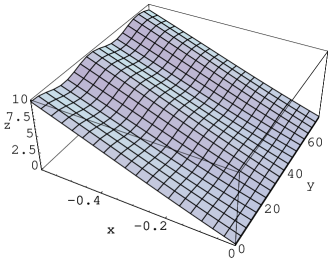
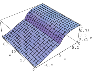
Figure 2: Perturbed front profile for the vortex and antivortex density field. The fronts propagate in the $x$ direction and has a sinusoidal modulation in the $y$ direction

As we have already mentioned in earlier sections, our linear stability analysis differs from the standard one, due to the presence of a singularity. The type of perturbation that we want to consider should not only involve the profile in the region where $n^{+}$ vanishes, but should also in particular involve the geometry of the front. In other words, as Fig. 2 illustrates, we want to perturb also the location of the singular line at which the density $n^{+}$ vanishes. As discussed in more detail in Judith , the proper way to implement this idea is to introduce a modulated variable

$$\zeta(\xi,y,t)=\xi+\epsilon e^{iqy+\omega t+i\Omega t}$$ (35)

and then to write the densities in terms of this “comoving” modulated variable. Of course, the proper coordinate is the real variable $\mbox{Re}\,\zeta$. However, when we expand the functions in Fourier modes and linearize the dynamical equations in the amplitude $\varepsilon$, each Fourier mode can be treated separately. Thus, we can focus on the single mode with wavenumber $q$ and amplitude $\epsilon$ and then take the real part at the end of the calculation. The profiles of the fields $n^{+}$ and $n^{-}$ are now perturbed by writing

$$n^{+}(\zeta,y,t) =n^{+}_{0}(\zeta)+\epsilon(n^{+}_{1}+in^{+}_{2})(\zeta)e^{iqy+\omega t+i\Omega t}$$ , (36)

$$n^{-}(\zeta,y,t) =n^{-}_{0}(\zeta)+\epsilon(n^{-}_{1}+in^{-}_{2})(\zeta))e^{iqy+\omega t+i\Omega t}$$ , (37)

where $n^{+}_{0}$ and $n^{-}_{0}$ are simply the planar front profiles determined before. Note that since we write these solutions as a function of the modulated variable $\zeta$, even the first term already implies a modulation of the singular line. Indeed, the standard perturbation ansatz would fail for our problem because of the singular behavior of the front. The usual ansatz of a stability calculation

$$n^{+}(\xi,y,t)=n^{+}_{0}(\xi)+\epsilon(n^{+}_{1}+in^{+}_{2})(\xi)e^{iqy+\omega t+i\Omega t}$$ (38)

only works if the unperturbed profiles are smooth enough and not vanishing in a semi-infinite region. If we impose on our corrected linear stability analysis the conditions

$$\frac{n^{+}_{1}+in^{+}_{2}}{n^{+}_{0}}\hskip 8.5359pt\mbox{ bounded}\hskip 8.5359pt\mbox{and}\hskip 8.5359pt\frac{n^{-}_{1}+in^{-}_{2}}{n^{-}_{0}}\hskip 8.5359pt\mbox{ bounded}$$ (39)

then as $\varepsilon\to 0$ the perturbations can be considered small everywhere, plus we allow for a modulation of the singular line Judith .

We next linearize the equations (33) around the uniformly translating solution according to (36-37). We obtain a set of 4 linearized ODEs for the variables ${D_{1},D_{2},S_{1},S_{2}}$, which correspond, respectively, to the real and imaginary parts of the difference and sum variables introduced in (27). These equations, which are reported in the Appendix, depend also on the unperturbed profiles $D_{0},S_{0}$, which are known from the derivation in Section II.1. Moreover, there is an explicit dependence on the parameters $q,\omega,\Omega$.

In order to analyze the stability of the front of vortices and antivortices, the dispersion relation $\omega(q),\Omega(q)$ must be derived. This can be determined with a shooting method: for every wavenumber $q$ there is a unique value of the growth rate $\omega$ and frequency $\Omega$ which satisfies the boundary conditions related to the perturbed front. If the growth rate is positive, a small perturbation will grow in time, thus leading to an instability.

III.3 The shooting method

The singularity of the front makes the numerical integration difficult to handle, as in the case of the planar front. In view of the relations (39), the boundary conditions

$$n^{+}_{1}=0,\mbox{\hskip 28.45274pt}n^{+}_{2}=0,$$

have to be imposed for $\zeta=0$. These yield the boundary conditions for the variables $D_{1},S_{1},D_{2},S_{2}$

$$S_{1}=-D_{1},\mbox{\hskip 28.45274pt}S_{2}=-D_{2}.$$ (40)

Moreover, by substituting these boundary conditions and the relations (21) for the unperturbed fields in the linearized equations for ${D_{1},D_{2},S_{1},S_{2}}$, the following relations can be derived for $\zeta$ vanishing from the left note5 :

$$\left.\frac{dD_{1}}{d\zeta}\right|_{0^{-}} = \omega+qkD_{2}(0),$$ (41)

$$\left.\frac{dD_{2}}{d\zeta}\right|_{0^{-}} = \Omega-qkD_{1}(0)-\left.2qk\frac{dD_{0}}{d\zeta}\right|_{0^{-}}.$$ (42)

An explicit expression for the derivative of the sum of the real and imaginary part of the perturbations $S_{1},S_{2}$ can also be derived from the equations reported in the Appendix. In particular, these have the following generic form

$$\frac{dS_{1}(\zeta)}{d\zeta}=\frac{{\cal N}_{1}(\zeta)}{{\cal D}_{1}(\zeta)},\mbox{\hskip 28.45274pt}\frac{dS_{2}}{d\zeta}=\frac{{\cal N}_{2}(\zeta)}{{\cal D}_{2}(\zeta)},$$ (43)

which is similar in structure to Eqs. (30): ${\cal N}_{1},{\cal D}_{1},{\cal N}_{2},{\cal D}_{2}$ depend on $\zeta$ through the set of functions

$$\left(D_{0},S_{0},\frac{dD_{0}}{d\zeta},\frac{dS_{0}}{d\zeta},D_{1},S_{1},\frac{dD_{1}}{d\zeta},D_{2},S_{2},\frac{dD_{2}}{d\zeta}\right),$$

and on the parameters $q,\omega,\Omega$.

The equations (43) are not defined at the singular point. By substituting the boundary conditions given by (40-42), both the numerators ${\cal N}_{1},{\cal N}_{2}$ and the denominators ${\cal D}_{1},{\cal D}_{2}$ vanish. Again, as with (30), we encounter the problem of dealing with the singularity at $\zeta=0$. This difficulty can be overcome in the same way as in Section II.2 for the derivation of the planar front profile. In particular, we can not start the integration at the singular point, but we have to start the backwards integration at some small distance on the left of $\zeta=0$. We do so by first obtaining the derivatives of the fields $S_{1}$ and $S_{2}$ analytically through the expansion of the equations (43) around the critical point. In the limit $\zeta\rightarrow 0$, this yields the following self-consistency condition for the derivatives.

$$\left.\frac{dS_{1}}{d\zeta}\right|_{0^{-}}=\frac{{\cal N}^{\prime}_{1}|_{0^{-}}}{{\cal D}^{\prime}_{1}|_{0^{-}}},\mbox{\hskip 14.22636pt}\left.\frac{dS_{2}}{d\zeta}\right|_{0^{-}}=\frac{{\cal N}^{\prime}_{2}|_{0^{-}}}{{\cal D}^{\prime}_{2}|_{0^{-}}},$$ (44)

where ${\cal N}^{\prime}_{1},{\cal N}^{\prime}_{2},{\cal D}^{\prime}_{1},{\cal D}^{\prime}_{2}$ denote the derivatives of the corresponding functions evaluated at the singular point. Once these are solved and used in the numerics, the integration can be carried out smoothly.

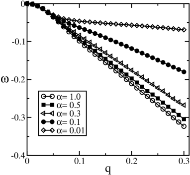
Figure 3: Dispersion relation $\omega(q)$ for different values of anisotropy coefficient $\alpha$ and a velocity $v=1.0$.

Because of the singularity at the point $\zeta=0$, the derivative of the perturbed fields are not continuous there and a relationship for the discontinuity in the derivatives can be derived as was the case for the unperturbed fields. In particular, the expression (15) is generalized for the perturbed field. This implies that the derivative of the total magnetic field is again continuous even at the singularity.

From the equations for the perturbed fields given in the Appendix, the boundary conditions at $\xi=-L$ can be derived. Just like the unperturbed field for the antivortex density vanishes on the left with a Gaussian behaviour according to (13), also the perturbations $n_{1}^{-}$ and $n_{2}^{-}$ vanish as a Gaussian, i.e. faster then an exponential.

Moreover, since the density of vortices increases linearly asymptotically, we can retain in the equations only terms which are proportional to the density of vortices $n_{0}^{+}$. From this we get the following equation for the density of the perturbation $\delta n^{+}=n_{1}^{+}+in_{2}^{+}$ for $\zeta\ll-1$

$$\frac{d^{2}\delta n^{+}}{d^{2}\zeta}+2iqk\frac{d\delta n^{+}}{d\zeta}-pq^{2}\delta n^{+}=pq^{2}\frac{dn_{0}^{+}}{d\zeta}.$$ (45)

The solutions of this equation which do not diverge are of the form

$$\delta n^{+}=-\frac{dn_{0}^{+}}{d\zeta}+Ce^{\lambda\zeta},\hskip 5.69046pt\lambda=iqk+\sqrt{(q^{2}(p-k^{2}))},$$ (46)

where $C$ is an arbitrary constant and $k$ and $p$ represent the coefficients of anisotropy defined in (34). Thus, the perturbations decay on the left of the film with a decay length $\zeta_{0}$, such that

$$\frac{1}{\zeta_{0}}=q\sqrt{p-k^{2}}.$$ (47)

Note that the decay length becomes very large for small $q$; this type of behavior is of course found generically in diffusion limited growth models. Technically it means that we need to be careful to take large enough systems to study the small-$q$ behavior. From the numerical integration it was verified that Eqs. (46) and (47) describe correctly the behavior of $\delta n^{+}$ at large distance.

Figure 4: Imaginary part of the growth rate $\Omega(q)$ for different values of the anisotropy coefficient $\alpha$, with velocity $v=1.0$.

Furthermore, since vortices are absent in the positive region, we have to impose that the density of the perturbation related to the $n^{+}$ field, and its derivative in space, have to vanish there. Similarly we get a second ODE with constant coefficients by considering that the density of antivortices is constant at large positive distances. Taking again $n^{-}_{\infty}=1$, we get, for $\zeta\gg 1$:

$$\frac{d^{2}\delta n^{-}}{d^{2}\zeta}+(v+2iqk)\frac{d\delta n^{-}}{d\zeta}-(pq^{2}+\omega+i\Omega)\delta n^{-}=0.$$ (48)

In order to satisfy the boundary condition, we must consider the solution which vanishes exponentially. The solution of this equation which does not diverge is of the form

$$\delta n^{-}=C_{1}e^{\bar{\lambda}\zeta}\hskip 5.69046pt,Re(\bar{\lambda})<0.$$ (49)

We applied the shooting method in a 4-dimensional space defined by the free parameters $D_{1}(0),D_{2}(0),\omega$ and $\Omega$, by integrating backward in the interval $[-L,0]$ and then in $[0,+\infty[$, looking for solutions of the type (46,49).

By matching the solutions to the boundary conditions

$$\begin{array}[]{ll}\displaystyle\lim_{\zeta\rightarrow-L}n_{1}^{+}=-\frac{dn_{0}^{+}}{d\zeta}.&\displaystyle\lim_{\zeta\rightarrow-L}n_{2}^{+}=0,\\ \displaystyle\lim_{\zeta\rightarrow+\infty}n_{1}^{-}=0,&\displaystyle\lim_{\zeta\rightarrow+\infty}n_{2}^{-}=0,\end{array}$$ (50)

we then obtain a unique dispersion relation for the real part of the growth rate $\omega(q)$.

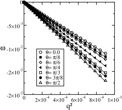
Figure 5: (a) Plot of $\omega(q^{2})$ as a function of the angle $\theta$. (b) For a coefficient of anisotropy $\alpha=0.8$ and a velocity $v=1.0$, the results from linear regression for the slope evaluated at $q=0$, $c=d\omega/d(q^{2})$, are plotted as a function of $\theta$.

III.4 Results

Fig. 3 represents the dispersion relation for an angle $\theta=\pi/4$ and different coefficients of anisotropy $\alpha$. The front is always stable, even in the presence of very strong anisotropy, for very low values of $\alpha$. As the anisotropic coefficient $\alpha$ is lowered from above, for fixed wavenumber $q$, the growth rate $\omega(q)$ increases, but it is always negative. For small $q$ a quadratic behavior of $\omega(q)$ is found:

$$\omega\approx cq^{2},\hskip 5.69046ptq\ll 1,$$ (51)

where the (negative) coefficient $c$ depends on the anisotropy of the sample. In Fig. 4 we have plotted the frequency $\Omega$ as a function of the wavenumber $q$. One observes from (35) that $\Omega/q$ is the velocity with which the perturbation of the front shifts along the direction transverse to the propagation direction. The behavior of $\Omega(q)$ is linear for low wavenumber $q$ and is proportional to the non-diagonal element of the mobility tensor $k$,

$$\Omega(q)\propto kq,\hskip 5.69046ptq\ll 1.$$ (52)

For an anisotropy coefficient equal to one the isotropic case is recovered and then $\Omega(q)$ vanishes identically for all wavenumbers. As we have already mentioned, the equations that we have used are valid at scales larger than the cutoff represented by the London penetration depth. Anyway, since our results clearly show a stability in the large $q$ behavior, our model provides a good description for the dynamics of the front. In Fig. 5 we plot the growth rate $\omega$ as a function of $q^{2}$ for different values of the angle $\theta$. Linear regression then gives a slope corresponding to the constant $c$ in (51), which is half the second derivative of the growth rate $\omega$ with respect the wavenumber at $q=0$. The dependence of $c$ as a function of the angle $\theta$ is shown in the lower plot. As the angle $\theta$ increases, the front becomes more and more stable. This behavior can be understood directly from the form of the equations. By applying the transformation

$$\theta\rightarrow\displaystyle{\frac{\pi}{2}}-\theta,\hskip 5.69046pt0<\theta<\pi/4,$$ (53)

the elements of the mobility tensor transform into

$$p\rightarrow{\displaystyle\frac{1}{p}},\mbox{\hskip 14.22636pt}k\rightarrow{\frac{k}{p}}.$$ (54)

By considering the quadratic relation of $\omega(q)$ for small $q$ and the fact that the equations are invariant under the transformations $\tilde{q}=pq$ and (54), it is easy to derive

$$\omega(q)|_{{\theta}}=p^{2}\omega(q)|_{{\pi/2-\theta}},\hskip 5.69046pt0<p<1,$$ (55)

which proves that the dispersion relation becomes more negative as $\theta$ increases. When the direction of propagation is that of the fast growth direction the isotropic case is recovered.

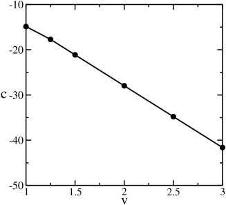
Figure 6: Velocity dependence of half the second derivative of $\omega(q)$ with respect to $q$ evaluated at $q=0$. As the velocity increases the front becomes more and more stable.

In Fig. 6 we show the dependence of the coefficient $c$ as a function of the velocity of the front. The front is stable for velocities for which $n^{+}_{0}$ vanishes linearly ($v\geq 1/4$). Furthermore the front becomes more stable with increasing $v$. As one can easily understand from the form of the unperturbed front, the vortex density profile becomes steeper with increasing the velocity. The limit of infinitely large $v$ corresponds to the case of a front of vortices propagating in the absence of antivortices. Thus, the results confirm the stability of the front without an opposing flux of antivortices.

IV Stationary front

Figure 7: Density profiles for vortices and antivortices in the stationary case ($v=0$). The profiles are smooth and are not characterised by singularities, as was the case for fronts propagating with finite velocity.

As we mentioned in the introduction, we have also analysed the case of a stationary front, with $v=0$. In this case it is easy to derive the unperturbed profiles for the densities of vortices and antivortices, since they are continuous and do not present any singularities. This case was previously studied in (Fisher ) and treated in terms of a sharp interface limit. Equations (9,10) in this case simplify to:

$$\frac{d}{d\xi}n_{0}^{+}\,\frac{d}{d\xi}(n_{0}^{+}-n_{0}^{-})-n_{0}^{+}n_{0}^{-} = 0,$$ (56)

$$\frac{d}{d\xi}n_{0}^{-}\,\frac{d}{d\xi}(n_{0}^{-}-n_{0}^{+})-n_{0}^{+}n_{0}^{-} = 0.$$ (57)

The profiles of vortices and antivortices are symmetric in this case, and outside the interfacial zone the density fields can be easily derived analytically. By neglecting the annihilation term, the profiles of vortices and antivortices have a dependence on the coordinate $\xi$ of the type:

$$n_{0}^{\pm}=\sqrt{N^{2}\mp 2C(\xi\pm\xi_{1})},$$ (58)

where $]-\xi_{1},\xi_{1}[$ denotes the region where vortices and antivortices overlap, N is the density at $(\pm\xi_{1})$ and C a constant. The density of vortices and antivortices decays with a Gaussian tail, as can easily be calculated from equations (56 and 57). For Eq. (56), by considering that $n_{0}^{+}$ assumes a Gaussian-like dependence, and from the form of (58), we get the following equation:

$$-\frac{dn_{0}^{+}}{d\xi}\frac{dn_{0}^{-}}{d\xi}=n_{0}^{+}n_{0}^{-}.$$ (59)

This yields in a self-consistent way a Gaussian behaviour for $n^{+}$:

$$n_{0}^{+}\approx Ae^{-\xi^{2}-\xi(N^{2}/C-2\xi_{1})},$$ (60)

where $A$ is a constant. The density profiles for vortices and anti-vortices are represented in Fig.7. The stability of the front was studied by following a similar procedure as for the moving front. Because of the regular profiles, the ansatz (35) that we have applied for the case of a finite velocity is not required. Thus the linear stability analysis can be carried out in the standard way and the linearised equations for the perturbation can easily be integrated. We do not explain here the procedure in detail, since it is a simplified version of the one discussed in the previous section.

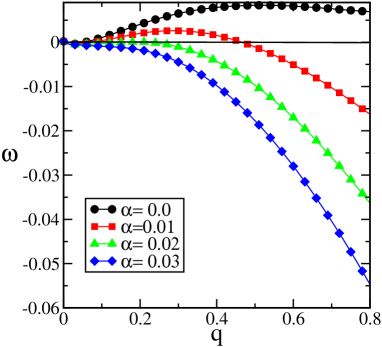
Figure 8: Dispersion relation $\omega(q)$ in the case of a stationary front. An instability is found for a critical anisotropy coefficient $\alpha_{c}\approx 0.02$.

As Fig. 8 shows, an instability is found below a critical coefficient of anisotropy $\alpha_{c}\approx 0.02$. These results confirm previous approximate calculations Fisher , but, as we have already underlined, this coefficient would correspond to an extremely high in-plane anisotropy which is not found in any type of superconducting material. We conclude that this model of a stationary front in the presence of anisotropy is insufficient to explain the turbulent behaviour that has been found experimentally at the flux-antiflux boundary.

V Conclusions

From our analysis it follows that the planar front of vortices moving with a sufficiently large velocity $v$ in a superconducting thin film is stable even in the presence of strong in-plane anisotropy. For stationary fronts, on the other hand, our stability analysis confirms the earlier approximate analysis of Fisher , confirming that such fronts show an instability to a modulated state in the limit of very strong anisotropy. From an experimental point of view, the critical anisotropy of this instability is very high when compared with real values that can be found for materials with both tetragonal and orthorhombic structure anisocoeff2 ; anisocoeff3 , even when a non-linear current-electric field characteristic is considered Fisher1 . From a theoretical point of view, the behavior in the limit of small but finite $v$ is still open as we have not investigated the range $0<v<1/4$ where the profiles have a noninteger power law singularity. It could be that the instability gradually becomes suppressed as $v$ increases from zero, or it could be that the limit $v\to 0$ is singular, and that moving fronts are stable for any nonzero $v$. Only further study can answer this question.

Our calculations differ markedly from previous work in that we focus on moving fronts from the start, where our results follow from a straightforward application of linear stability analysis to our model. Taken together, these results lead to the conclusion that a model which includes a realistic in-plane anisotropy, but which neglects the coupling with the temperature, cannot explain the formation of an instability at a vortex-antivortex boundary for sufficiently large front velocities. At the same time, our calculations show that the issue of the stability of vortex fronts is surprisingly subtle and rich. For example, we note the fact that for any front velocity, the value $n^{-}_{0}$ at the singular line is exactly $n_{\infty}/2$ for any $v$. Is this simply a mathematical curiosity or is the absence of instabilities related to this unexpected feature through the boundary conditions at infinity? Is the presence of a gradient in the antivortex distribution far ahead of the front perhaps necessary to generate a long-wavelength front instability? These are all still open issues, so clearly it is difficult to make general statements about the (transient) stability of such fronts in less idealized situations.

One possible interpretation of the results is that when one has a finite slab into which vortices penetrate from one side, and antivortices from the other side, a stationary modulated front (anihilation zone) forms in the middle for extremely large anisotropies. However, a moving front never has a true Mullins-Sekerka type instability, since a protrusion of the front into the region of antivortices is always damped as a result of the increased annihilation.

The fact that the turbulent behavior at the interface between vortices of opposite sign was found in a temperature window Koblischka , shows that the coupling with the local temperature in the sample has to be considered. It appears that it is necessary to include both the heat transport and dissipation in the model. Applying an appropriate stability analysis to such extended models is clearly an important issue for the future.

VI Acknowledgment

We are grateful to Hans de Haan for performing time-dependent simulations of the one-dimensional vortex dynamics equations, which showed that we were initially mistaken about the nature of the induced singularities in the $n^{-}$ field. In addition we have profited from discussions with Peter Kes, Rinke Wijngaarden and Gianni Blatter. C.B. is supported by the Dutch research foundation FOM, and would also like to thank the “Fondazione A. Della Riccia” and “Fondazione ing. A. Gini” for additional financial support. M.H. acknowledges financial support from The Royal Society.

Appendix A Linearized equations for the perturbed front

From the linear stability analysis we get the linearized equations for the variables $D$ and $S$:

$$\omega\left(D_{1}+\frac{dD_{0}}{d\zeta}\right)-\Omega D_{2}+pq^{2}S_{0}\left(D_{1}+\frac{dD_{0}}{d\zeta}\right)=$$ (61)

$$+v\frac{dD_{1}}{d\zeta}+\left(\frac{dS_{0}}{d\zeta}\right)\left(\frac{dD_{1}}{d\zeta}\right)+\left(\frac{dD_{0}}{d\zeta}\right)\left(\frac{dS_{1}}{d\zeta}\right)$$

$$+S_{0}\frac{d^{2}D_{1}}{d\zeta^{2}}+S_{1}\frac{d^{2}D_{0}}{d\zeta^{2}}-qk\left[2S_{0}\frac{dD_{2}}{d\zeta}+\frac{dS_{0}}{d\zeta}D_{2}+\frac{dD_{0}}{d\zeta}S_{2}\right]$$

$$\omega D_{2}+\Omega\left(D_{1}+\frac{dD_{0}}{d\zeta}\right)+pq^{2}S_{0}D_{2}=$$ (62)

$$+v\frac{dD_{2}}{d\zeta}+\left(\frac{dS_{0}}{d\zeta}\right)\left(\frac{dD_{2}}{d\zeta}\right)+\left(\frac{dD_{0}}{d\zeta}\right)\left(\frac{dS_{2}}{d\zeta}\right)$$

$$+S_{0}\frac{d^{2}D_{2}}{d\zeta^{2}}+S_{2}\frac{d^{2}D_{0}}{d\zeta^{2}}+qk\left[2S_{0}\left(\frac{dD_{1}}{d\zeta}+\frac{d^{2}D_{0}}{d\zeta^{2}}\right)\right.$$

$$+\left.\frac{dS_{0}}{d\zeta}\left(D_{1}+\frac{dD_{0}}{d\zeta}\right)+\frac{dD_{0}}{d\zeta}\left(S_{1}+\frac{dS_{0}}{d\zeta}\right)\right]$$

$$\omega\left(S_{1}+\frac{dS_{0}}{d\zeta}\right)-\Omega S_{2}+pq^{2}D_{0}\left(D_{1}+\frac{dD_{0}}{d\zeta}\right)=$$ (63)

$$+v\frac{dS_{1}}{d\zeta}+2\left(\frac{dD_{0}}{d\zeta}\right)\left(\frac{dD_{1}}{d\zeta}\right)+D_{0}\frac{d^{2}D_{1}}{d\zeta^{2}}$$

$$+D_{1}\frac{d^{2}D_{0}}{d\zeta^{2}}-qk\left[2D_{0}\frac{dD_{2}}{d\zeta}+2\frac{dD_{0}}{d\zeta}D_{2}\right]-S_{0}S_{1}+D_{0}D_{1}$$

$$\omega S_{2}+\Omega\left(S_{1}+\frac{dS_{0}}{d\zeta}\right)+pq^{2}D_{0}D_{2}=$$ (64)

$$+v\frac{dS_{2}}{d\zeta}+2\left(\frac{dD_{0}}{d\zeta}\right)\left(\frac{dD_{2}}{d\zeta}\right)+D_{0}\frac{d^{2}D_{2}}{d\zeta^{2}}+D_{2}\frac{d^{2}D_{0}}{d\zeta^{2}}$$

$$+qk\left[2D_{0}\left(\frac{dD_{1}}{d\zeta}+\frac{d^{2}D_{0}}{d^{2}\zeta}\right)+2\frac{dD_{0}}{d\zeta}\left(D_{1}+\frac{dD_{0}}{d\zeta}\right)\right]$$

$$-S_{0}S_{2}+D_{0}D_{2}$$

References

- (1) G. Blatter, M. V. Feigel’man, V. B. Geshkenbein, A. I. Larkin and V. M. Vinokur, Rev. Mod. Phys. 66, 1125 (1994).
- (2) G. Blatter and V. B. Geshkenbein, Vortex matter in: The physics of Superconductors, vol. 1, pp. 726-936, eds. K. H. Bennemann and K. Emerson (Springer, Berlin, 2003).
- (3) C. A. Duran, P. L. Gammel, R. E. Miller, and D. J. Bishop, Phys. Rev. B 52, 75 (1995).
- (4) T. H. Johansen, M. Baziljevich, D. V. Shantsev, P. E. Goa, Y. M. Galperin, W. N. Kang, H. J. Kim, E. M. Choi, M.-S. Kim, S. I. Lee, Europhysics Lett., 59, 599 (2002).
- (5) F. L. Barkov, D. V. Shantsev, T. H. Johansen, P. E. Goa, W. N. Kang, H. J. Kim, E. M. Choi and S.I. Lee, Phys. Rev. B 67, 064513 (2003)
- (6) M. Marchevsky, L. A. Gurevich, P. H. Kes, and J. Aarts, Phys. Rev. Lett. 75, 2400 (1995).
- (7) P. Leiderer, J. Boneberg, P. Brüll, V. Bujok and S. Herminghaus, Phys. Rev. Lett. 71, 2646 (1993).
- (8) R. Surdeanu, R. J. Wijngaarden, E. Visser, J. M. Huijbregtse, J. Rector, B. Dam and R. Griessen, Phys. Rev. Lett. 83, 2054 (1999).
- (9) W. W. Mullins and R. F. Sekerka, J. Appl. Phys. 34, 323 (1963)
- (10) T. Frello, M. Baziljevich, T. H. Johansen, N. H. Andersen, Th. Wolf, and M. R. Koblischka, Phys. Rev B, 59, R6639 (1999).
- (11) M. V. Indebom, H. Kronmüller, P. Kes and A. A. Menovsky, Physica C 209, 259 (1993).
- (12) M. R. Koblischka, T. H. Johansen, M. Baziljevich, H. Hauglin, H. Bratsberg and B. Y.Shapiro, Europhys. Lett. 41, 419 (1998).
- (13) V. K. Vlasko-Vlasov, V. I. Nikitenko, A. A. Polyanskii, G. V. Crabtree, U. Welp and B. W. Veal, Physica C 222, 361 (1994).
- (14) G. R. Mints and A. L. Rachmanov, Rev. Mod. Phys. 53, 551 (1981).
- (15) I. Aranson, A. Gurevich, and V. Vinokur, Phys. Rev. Lett. 87, 067003 (2001).
- (16) F. Bass, B. Ya. Shapiro, and M. Shvartser, Phys. Rev. Lett 80, 2441 (1998).
- (17) L. M. Fisher, P. E. Goa, M. Baziljevich, T. H. Johansen, A. L. Rakhmanov and V. A. Yampol’skii, Phys. Rev. Lett. 87, 247005 (2001).
- (18) A. L. Rakhmanov, L. M. Fisher, A. A. Levchenko, V. A. Yampol’skii, M. Baziljevich, and T. H. Johansen, JETP Letters, 76, 291 (2002).
- (19) G. J. Dolan, F. Holtzberg, C. Feild, and T. R. Dinger, Phys. Rev. Lett. 62, 2184 (1989).
- (20) K. Zhang, D. A. Bonn, S. Kamal, R. Liang, D. J. Baar, W. N. Hardy, D. Basov, and T. Timusk., Phys. Rev, Lett. 73, 2484 (1994).
- (21) C. A. Murray, P. L. Gammel, D. J. Bishop, D. B. Mitzi and A. Kapitulnik, Phys. Rev. Lett. 64, 2312 (1990).
- (22) P. G. Drazin and W. H. Reid, Hydrodynamic stability, (Cambridge University Press, Cambridge, 1981).
- (23) C. P. Bean, Rev. Mod. Phys. 36, 31 (1964).
- (24) J. Bear, Dynamics of Fluids in Porous Media (Elsevier, New York, 1972).
- (25) L. A. Peletier, in Application of Nonlinear Analysis in the Physical Sciences, H. Amman, N. Bazley and K. Kirchgaessner, eds. (Pitman, London, 1981).
- (26) The similarity between the nonlinear diffusion equation of vortices and the porous medium equation was pointed out in particular by J. Gilchrist and C. J. van den Beek, Physica C 231, 147 (1994).
- (27) V. M. Vinokur, M. V. Feigel’man and V. B. Geshkenbein, Phys. Rev. Lett. 67 915 (1991); H. G. Schnack and R. Griessen, Phys. Rev. Lett. 68 2706 (1992); V. M. Vinokur and V.B. Geshkenbein, Phys. Rev. Lett. 68 2707 (1992).
- (28) I. Golding, Y. Kozlovsky, I. Cohen, and E. Ben-Jacob, Physica A 260, 510 (1998).
- (29) J. Müller and W. van Saarloos, Phys. Rev. E 65, 061111 (2002).
- (30) In the nomenclature of G. I. Barenblatt, Similarity, Self-Similarity and Intermediate Asymptotics (Consultants Bureau, New York, 1979), this corresponds to a transition from self-similarity of the first kind to self-similarity of the second kind as a function of the front velocity.
-
(31)
We assume for the viscosity the Bardeen-Stephen relation
, with resistivity of
the material in the normal state.
J. Bardeen and M. J. Stephen, Phys. Rev. 140, A1197 (1965). - (32) C. M. Bender and S. A. Orzsag, Advanced Mathematical Methods for Scientists and Engineers (McGraw-Hill, New York, 1978).
- (33) In mathematical terms the field has compact support.
- (34) To simplify the presentation, we have included only the terms we need for our discussion. One can generalize the analysis by including regular terms with integer exponents, but the analysis then shows that these terms have to be absent if is non-integer.
- (35) Actually, since the jump in the derivative of is equal to the jump in the derivative of (compare Eq. (15), the derivatives of and are unique at . The derivative of has a jump, however.