Vison gap in the Rokhsar–Kivelson dimer model on the triangular lattice

Abstract

With the classical Monte Carlo method, I find the energy gap in the Rokhsar–Kivelson dimer model on the triangular lattice. I identify the lowest excitations as visons, and compute their energy as a function of the momentum.

The Rokhsar–Kivelson (RK) dimer model is an interesting example of a two-dimensional quantum liquid [1, 2, 3]. When the kinetic and potential coupling constants of the RK dimer model are equal (the so-called “RK point”), the ground state of the model is known exactly, and the ground-state properties on planar lattices may be analytically studied with the Pfaffian method [4]. Much attention was paid to the study of the RK model on the triangular lattice, in which case the RK point is known to be in the liquid phase with topological order and with exponentially decaying correlations [2, 5, 6] (on the square lattice, in contrast, the RK point has power-law correlations and a gapless spectrum, due to the bipartite nature of the lattice [1, 3, 7, 8, 9]). Unfortunately, our knowledge of the excitation spectrum at the RK point on the triangular lattice is limited to numerical methods [2, 10]. Studying excitations in the RK model is interesting in view of the prediction that the elementary excitations are the so-called “visons” which are non-local objects in terms of dimers. Visons were proposed as elementary excitations in quantum liquids with $Z_{2}$ gauge symmetry (possibly also in spin-1/2 systems)[11, 12]. While applicability of this proposal to realistic spin-1/2 systems is debatable, there exist model systems, where the existence of vison excitations is explicitly shown and the whole spectrum of visons may be exactly found [13, 14]. The usual price to pay for the exact solvability is that in such models the vison excitations are strictly local (i.e., their energy is independent of the momentum) and non-interacting. In contrast, the RK model presents a very non-trivial case, where the visons have their dispersion and interact in many-vison states.

In this work, I use the proposal of Henley to extract the energy gap of the excitations from the time correlation of the classical Monte Carlo algorithm used to compute the ground-state observables [9] (the classical calculation of the excitation spectrum is actually possible due to the supersymmetry of the RK point [15]; the relation between supersymmetric quantum systems and stochastic classical dynamics was discussed in various contexts [16]). By choosing appropriate correlation functions, we can resolve the momentum-dependence of the gap, and also distinguish excitations carrying odd number of visons from those carrying even number of visons. We find that the low-energy excitations are indeed vison-like (carry odd number of visons) and plot their dispersion in the Brillouin zone.

The Rokhsar–Kivelson dimer model may be defined on any graph: the dimer coverings of the graph define an orthonormal basis of the Hilbert space; and the quantum Hamiltonian is

$$H_{RK}=\sum\Big{(}-t\left|\lower 2.15277pt\hbox{ \epsfbox{fig-hor.eps}}\,\,\right\rangle\left\langle\lower 2.15277pt\hbox{ \epsfbox{fig-vert.eps}}\,\,\right|+v\left|\lower 2.15277pt\hbox{ \epsfbox{fig-hor.eps}}\,\,\right\rangle\left\langle\lower 2.15277pt\hbox{ \epsfbox{fig-hor.eps}}\,\,\right|\Big{)}$$ (1)

The sum is taken over all length-four loops of the graph. The two coupling constants $t$ and $v$ determine the strength of kinetic and potential terms, respectively. At the “RK point” $t=v$, the Hamiltonian can be shown to be non-negative (assuming $t>0$), and its ground state may be constructed as the sum of all dimer configurations taken with equal amplitudes (more precisely, we can restrict the sum to the dimer configurations from any connected component of the “phase space”, i.e. to configurations which can be obtained from each other by the kinetic term in the Hamiltonian (1)) [1]. This ground state has energy zero, which is a manifestation of the supersymmetry of the RK point [15]. We further specify to the case of the underlying graph being the two-dimensional triangular lattice (the sum in the Hamiltonian (1) is taken over all rhombi, so the total number of terms in the sum is three times the number of lattice sites), and set the energy units $t=v=1$. Our main objective in this paper is finding the low-lying excitations of this model. From earlier numerical studies, it has been suggested that this model has a gapped spectrum [2, 10], which seems to be in agreement with the exponential decay of ground-state correlation functions known from analytic studies [2, 5, 6].

From the general discussions of the dimer liquids in two dimensions, the $Z_{2}$-vortex operator (the so called “vison”) is known to play an important role among physical observables. The vison (more precisely, the “two-vison”) operator $V_{\Gamma}$ is defined for any contour $\Gamma$ intersecting links of the lattice and terminating either at the lattice boundary or inside a plaquet in the bulk of the lattice (Fig. 1a). The operator $V_{\Gamma}$ is defined as the parity of the number of dimers intersecting $\Gamma$:

$$V_{\Gamma}=(-1)^{{\rm no.~{}of~{}dimers~{}intersecting~{}}\Gamma}.$$ (2)

If one commutes such an operator with the Hamiltonian (1), the only non-vanishing contribution comes from the rhombi containing the end points of the contour. In particular, if the contour forms a closed loop or terminates at a lattice boundary, the corresponding operator exactly commutes with the Hamiltonian and gives rise to different topological sectors of the Hilbert space [1, 11, 17].

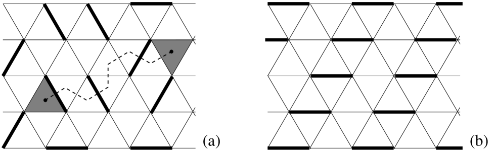
FIG. 1.: (a) Definition of the vison operator $V_{\Gamma}$. The contour $\Gamma$ (dashed line) connects two triangular plaquets of the lattice (shaded). The value of $V_{\Gamma}$ is the parity of the intersection of dimers with $\Gamma$. For the contour $\Gamma$ and for the dimer configuration shown in the figure, $V_{\Gamma}=-1$ (three intersections). (b) The reference dimer configuration for the sign fixing of a single-vison operator. An alternative (to that described in the main text) formulation of the sign-fixing rule: the contours $\Gamma$ must be drawn in such a way that they do not intersect dimers from the reference configuration.

It is natural to suggest that terminating the contour in the bulk of the lattice produces an excited state close to an eigenstate. Of course, to form a true excited eigenstate would require some “dressing” of the vison operator with local corrections around the contour end point. However, the topological structure of the excitation will be preserved vison-like. To clarify the above reasoning, we first describe some properties of the vison operators $V_{\Gamma}$. First, it is easy to check that the operator $V_{\Gamma}$, up to a sign, depends only on the end points of the contour; the dependence on the contour itself reduces to a controllable change of the sign: changing from the contour $\Gamma$ to another contour $\Gamma^{\prime}$ with the same end points changes the sign of the vison operator as $V_{\Gamma}=(-1)^{S}V_{\Gamma^{\prime}}$, where $S$ is the number of lattice points between the contours $\Gamma$ and $\Gamma^{\prime}$. Second, concatenation of the contours corresponds to the multiplication of the corresponding vison operators. Therefore we may represent the operator $V_{\Gamma}$ as the product of two vison operators at end points: $V_{\Gamma}=V_{1}V_{2}$, where each of the “single-vison” operators $V_{1}$ and $V_{2}$ depends on one of the two end points of $\Gamma$. Constructed this way, the point vison operators $V_{i}$ obey $Z_{2}$ algebra ($V_{i}^{2}=1$) and are defined on the frustrated dual lattice: their index $i$ refers to a plaquet of the original lattice, and they change sign on going around one lattice site of the original lattice. For the triangular lattice, we should think of visons as living on the hexagonal lattice with the magnetic flux of half quantum per hexagon.

To establish a sign convention for visons, we need to fix a $Z_{2}$ gauge on the dual lattice. This can be most easily done by taking a certain (arbitrary, but fixed once forever) dimer configuration as a reference one. Then in the definition (2), we multiply the right-hand side by the same expression $V_{\Gamma}$ computed in the reference dimer configuration. With the new definition, $V_{\Gamma}$ becomes a single-valued function of the end points of $\Gamma$ (independent of the choice of the contour). In our calculation, we take the reference dimer configuration as shown in Fig. 1b (note an additional doubling of the unit cell).

An important property of the vison operator is that it is a non-local operator in terms of dimers. A single-vison operator $V_{i}$ in an infinite system involves the contour $\Gamma$ continued to infinity and hence corresponds to a change in the boundary conditions on the wave function at infinity. Namely, a circular permutation of dimers along a big closed contour encircling the “excitation region” reverses sign of the excitation with odd number of visons, but keeps the wave function unchanged for the excitation with even number of visons (Fig. 2). According to this criterion, we may classify any “localized” wave packet as either vison-like or non-vison-like. Non-vison-like excitations are expressed as local operators in terms of dimers. A vison-like excitation may be described as a non-vison-like (local) operator multiplied by a vison operator. Thus we naturally have two classes of excitations with a $Z_{2}$ grading: combining two vison-like excitations we obtain a non-vison like excitation, while combining a non-vison-like excitation with a vison-like excitation gives a vison-like excitation. Of course, with this construction it seems natural that vison-like excitations should be considered as “elementary” excitations, while non-vison-like excitations may be constructed as composite excitations from vison-like elementary excitations. In reality, however, it may happen that vison-like excitations are pushed high in energy, so that the low-lying physical excitations are all non-vison-like. In this paper I demonstrate that it is not the case at the RK point on the triangular lattice. We shall see that both the vison-like and non-vison-like sectors are gapped and that the gap in the vison-like sector is smaller than in the non-vison-like sector. So vison excitations are indeed the lowest-energy excitations in the model.

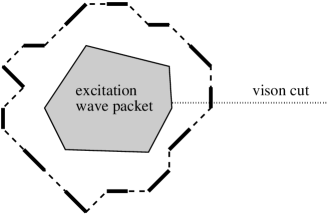
FIG. 2.: A localized wave packet of vison-like excitations. Vison-like excitations may be distinguished from non-vison-like ones by a circular permutation of dimers along a big contour (shown). If we denote such a permutation by $P$, vison-like excitations obey the equation $P^{2}=-P$, while non-vison-like excitations have $P^{2}=P$.

The exponentially decaying ground-state correlation functions [2, 5] suggest a gap in the excitation spectrum, and indeed both quantum Monte Carlo studies [2] and exact diagonalization on small systems [10] suggest the presence of the gap (from exact diagonalization, the value of the gap was estimated as 0.1). However, as pointed out by Henley [9], at the RK point the gap may be more easily extracted from a classical Monte Carlo simulation similar to that used for calculating the ground-state expectation values (see, e.g., Refs. [18, 6]). Namely, consider the following random walk defined on the space of all dimer coverings of the lattice. A step of the random walk is defined as picking at random any rhombus and, if it contains two parallel dimers, flipping this pair of dimers into the other two sides of the rhombus (as indicated by the kinetic term of the Hamiltonian (1)). If the chosen rhombus is non-flippable, the dimer configuration remains unchanged at this step of the random walk.

As shown by Henley [9], such a random walk simulates the quantum-mechanical evolution in imaginary time. Accordingly, the exponents governing the decay of the dynamic correlation functions with time are given precisely by the excitation energies of the quantum system. For our discrete random walk, this procedure of determining the excitation energies produces systematic errors arising from the discretization of time steps. The discreteness of time steps may, in principle, be properly compensated; however, we simply neglect the corresponding systematic errors. One can show that discretization of time leads to relative corrections to the gap magnitude of approximately one over the total number of rhombi in the system. In our Monte Carlo calculation we take a sufficiently large system of 20$\times$20 sites (thus containing 1200 rhombi), and those corrections are smaller than the statistical errors for the lengths of random walks used in our calculations. Therefore we disregard the time-discretization errors and extract the gaps directly from the correlations of the discrete random walk.

The next useful observation is that, by taking appropriate correlation functions, we can probe the gap at a given wave vector. And, moreover, we can distinguish between vison-like and non-vison-like excitation sectors. For computing the gap in the non-vison-like sector, we should consider correlations of non-vison-like observables (e.g., the dimer density). For the gap in the vison sector we take vison-like observables (e.g., the point vison $V_{i}$ defined above).

We first consider the excitations in the vison-like sector. In order to compute the gap, we take the correlation function

$$F({\bf r}_{ij},t-t^{\prime})=\langle V_{i}(t)V_{j}(t^{\prime})\rangle\,,$$ (3)

where $V_{i}(t)$ is the point vison on the triangle $i$ at the moment $t$ of the random-walk procedure as defined above, ${\bf r}_{ij}$ is the vector connecting the plaquets $i$ and $j$. This correlation function is properly defined, in spite of having only one vison operator at each of the time moments $t$ and $t^{\prime}$. To demonstrate the consistency of the definition (3), it is convenient to insert the square of the vison operator $[V_{j}(t)]^{2}=1$. Then we rewrite $V_{i}(t)V_{j}(t^{\prime})=(V_{i}(t)V_{j}(t))(V_{j}(t)V_{j}(t^{\prime}))$. The first product of the two vison operators is defined in (2) with the contour $\Gamma$ connecting the points $i$ and $j$. The second product involves two vison operators at one space point, but at different time moments. Obviously this product is also well defined for our random-walk process: namely, every dimer flip at any time between $t$ and $t^{\prime}$ on a rhombus containing the triangle $j$ changes the sign of $V_{j}(t)V_{j}(t^{\prime})$. In other words, $V_{j}(t)V_{j}(t^{\prime})$ counts the parity of the number of such flips.

FIG. 3.: This figure shows the Brillouin zones for non-vison-like and vison-like excitations (superimposed, on the same scale). Non-vison-like excitations: the Brillouin zone is the big hexagon (solid line; the side length of the hexagon is 4$\pi$/3 in the units of the inverse lattice constant of the original triangular lattice), with the minimum-gap points marked with big circles and labeled $\alpha$. Vison-like excitations: the Brillouin zone is the dashed rectangle (for the choice of gauge specified in Fig. 1b). The small solid circles, squares, and triangles (labeled with the letters $A$, $B$, and $C$, respectively) are the high-symmetry points. For example, points $A$ are centers of six-fold symmetry. The vison gap is found to reach its minimum at points $B$, and to increase strongly towards points $A$.

With the gauge choice for visons as discussed above (Fig. 1b), the unit cell of the lattice is doubled, and contains four triangular plaquets. To characterize vison excitations with wave vectors, we perform a Fourier transform of the correlation function (3) and arrive at the 4$\times$4 matrix $F({\bf k},t)$, where ${\bf k}$ is the wave vector from the reduced Brillouin zone. The full Brillouin zone and the reduced Brillouin zone are sketched in Fig. 3. Note that with our choice of the vison gauge, the correlation function $F({\bf k},t)$ has certain symmetries in the $k$-space reflecting the symmetries of the original triangular lattice. Those symmetries contain the six-fold rotation/reflection symmetry ($D_{6}$ symmetry group) around a certain point in the $k$-space, together with translations by two basis vectors defining a triangular lattice. The high-symmetry points in the $k$-space are marked in Fig. 3 by letters $A$, $B$, and $C$.

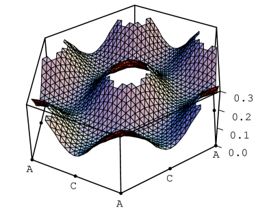
FIG. 4.: Top: the energy of the vison-like excitations along the section $A$–$B$–$C$–$A$ of the Brillouin zone shown in Fig. 3. The error bars are much smaller than the symbol size. The arrows on the energy axis indicate positions of $\Delta_{B}$ (bottom of the vison band), $\Delta_{0}$ (lowest-energy non-vison-like excitation), and $\Delta_{B}+\Delta_{0}$ (an estimate for the bottom of the three-vison continuum). Bottom: three-dimensional plot of the energy of the vison-like excitations as a function of the wave vector. The center and the corners of the hexagon correspond to the points $A$, as labeled in Fig. 3.

Now we determine the energy of the vison excitations $\Delta({\bf k})$ from the exponential decay of the diagonal elements of $F({\bf k},t)$ [19]. The sections of the energy dispersion along the “crystallographic axes” of the Brillouin zone and the 3-D plot of $\Delta({\bf k})$ are presented in Fig. 4. The points $B$ of the $k$-space give the minimal energy gap $\Delta_{B}=0.089(1)$ [which agrees with Ref. [10] claiming the gap value 0.1]. The points $C$ are the saddle points of the energy dispersion with $\Delta_{C}=0.114(1)$. The points $A$ are the centers of high-energy regions. In those regions, a naive fitting with an exponential suggests $\Delta_{A}>0.3$ and does not reproduce well the $t$-dependence of $F({\bf k},t)$. This may indicate that, at those wave vectors, the lowest excitations are not elementary visons, but rather combinations of three visons from the points $B$. Thus the $t$-dependence of $F({\bf k},t)$ reflects not an isolated excitation, but the bottom of a multi-particle continuum. The difference in the time dependence between low-energy and high-energy regions in the $k$ space is illustrated in Fig. 5 where we show typical $t$-dependences of $F({\bf k},t)$ for the two $k$-points: one near point $B$ in the $k$-space, and the other one near point $A$.

FIG. 5.: Typical vison and dimer correlations in the classical Monte Carlo random walk. Solid an dashed line show the vison correlations for wave vectors near points $B$ and $A$, respectively (see Fig. 3). Note that while near point $B$ the correlation function has a well-marked exponential behavior at long times, the correlations near point $A$ do not allow a precise fitting with a single exponent. The dotted line shows the dimer-dimer correlation function at the point $\alpha$ (the minimum-gap point). A good exponential decay of the correlation function possibly indicates a two-vison bound state.

Next, we repeat the same procedure for non-vison-like excitations by taking the correlations of the dimer-density operator instead of the vison operator $V_{i}(t)$ in (3). We then find that the lowest gap in the non-vison sector is $\Delta_{0}=0.144(1)$ and is reached at points labeled $\alpha$ in Fig. 3. The $t$-dependence of the dimer-dimer correlation function at point $\alpha$ is shown in Fig. 5. A good fit with an exponential dependence, together with the inequality $\Delta_{0}<2\Delta_{B}$, suggests that the lowest non-vison-like excitation is not just a superposition of two non-interacting vison excitations, but a bound state of such a pair. On the other hand, its energy is considerably higher than that of an elementary vison excitation ($\Delta_{B}$), which confirms the claim that the lowest excitation is vison-like. [This result also suggests to estimate the bottom of the continuum in the vison-like excitations as $\Delta_{0}+\Delta_{B}$ instead of $3\Delta_{B}$, see Fig. 4a.]

Finally, with this method of calculating the excitation gap, we can verify the claim of Ref.[10] about the absence of low-lying edge states in the case of lattices with boundaries. We examine the excitation spectrum of the 10$\times$10 and 20$\times$20 cylinders with straight boundaries along the lattice directions. From the result on non-vison-like excitations in the bulk, we expect that visons are attracted to each other, and therefore, visons should also get attracted to boundaries (since the vison cut may be terminated at the boundary at no energy cost). Note also that near the boundary there is no distinction between vison-like and non-vison-like excitations. Thus for determining the energy of the edge states we may take the dimer-dimer correlation function at the very boundary. Our classical Monte Carlo simulation gives the boundary gap $\Delta_{\rm edge}=0.072(1)$ reached at the wave vector $\pi$ along the boundary. In line with our expectations, the gap at the boundary is indeed somewhat reduced compared to the bulk vison gap, but remains finite.

The author thanks M. Feigelman for helpful discussions and comments.

REFERENCES

- [1] D. S. Rokhsar and S. A. Kivelson, Phys. Rev. Lett. 61, 2376 (1988).
- [2] R. Moessner and S. L. Sondhi, Phys. Rev. Lett. 86, 1881 (2001).
- [3] R. Moessner, S. L. Sondhi, and E. Fradkin, Phys. Rev. B 65, 024504 (2002) [cond-mat/0103396].
- [4] P. W. Kasteleyn, J. Math. Phys. 4, 287 (1963).
- [5] P. Fendley, R. Moessner, and S. L. Sondhi, Phys. Rev. B 66, 214513 (2002) [cond-mat/0206159].
- [6] A. Ioselevich, D. A. Ivanov, and M. V. Feigelman, Phys. Rev. B 66, 174405 (2002) [cond-mat/0206451].
- [7] M. E. Fisher and J. Stephenson, Phys. Rev. 132, 1411 (1963).
- [8] L. S. Levitov, Phys. Rev. Lett. 64, 92 (1990).
- [9] C. Henley, cond-mat/0311345.
- [10] L. B. Ioffe et al, Nature 415, 503 (2002); L. B. Ioffe, unpublished.
- [11] N. Read and B. Chakraborty, Phys. Rev. B 40, 7133 (1989).
- [12] T. Senthil and M. P. A. Fisher, Phys. Rev. B 62, 7850 (2000); ibid. 63, 134521 (2001).
- [13] G. Misguich, D. Serban, V. Pasquier, Phys. Rev. Lett. 89, 137202 (2002) [cond-mat/0204428].
- [14] L. B. Ioffe and M. V. Feigelman, Phys. Rev. B 66, 224503 (2002) [cond-mat/0205186].
- [15] M. V. Feigelman, unpublished.
- [16] M. V. Feigelman and M. A. Skvortsov, cond-mat/9703215; M. V. Feigelman and A. M. Tsvelik, ZhETF 83, 1430 (1982) [Sov. Phys. JETP 56, 823 (1982)]; J. Zinn-Justin, Quantum Field Theory and Critical Phenomena, Clarendon Press, Oxford (1993).
- [17] N. Bonesteel, Phys. Rev. B 40, 8954 (1989).
- [18] L. Balents, M. P. A. Fisher, and S. M. Girvin, Phys. Rev. B 65, 224412 (2002) [cond-mat/0110005].
- [19] The numerical results are obtained on the 2020 torus constructed by identifying sites spaced by 20 lattice constants in any of the three lattice directions. I combine the data from all the four topological sectors [6], which allows us to quadruple the number of accessible -points in the Brillouin zone. With the ground-state correlation length of order one lattice constant [5, 6], the finite-size effects on the spectrum may be neglected.