Efficient simulations of charged colloidal dispersions: A density functional approach

Abstract

A numerical method is presented for first-principle simulations of charged colloidal dispersions in electrolyte solutions. Utilizing a smoothed profile for colloid-solvent boundaries, efficient mesoscopic simulations are enabled for modeling dispersions of many colloidal particles exhibiting many-body electrostatic interactions. The validity of the method was examined for simple colloid geometries, and the efficiency was demonstrated by calculating stable structures of two-dimensional dispersions, which resulted in the formation of colloidal crystals.

I introduction

Electrostatic interactions play a crucial role in colloidal dispersions Israelachvili (1992); Russel et al. (1989); Safran (1994). When colloidal particles are immersed in electrolyte solutions, the so-called electric double layer is formed. The electric double layer is a cloud of counterions dissociated from the surfaces of the colloids into the solvent surrounding the colloidal particles. Most counterions are localized within the double layer due to the electrostatic attractive interactions between counterions and the inversely charged colloidal surfaces, while the entropy of the counterions tends to delocalize them. The thickness of the double layer is then determined by the competition between these conflicting effects. The static density profiles of the counterions can be calculated properly using the Poisson–Boltzmann theory, and its linearized version leads to the well-known screened Coulomb interaction for a pair of likely charged colloids. Although the screened Coulomb potential is widely used to simulate charged colloidal dispersions, the linearization is justified only for large interparticle separations. Deviations from screened Coulomb interaction become notable for the interparticle separation smaller than the Debye screening length. Furthermore, many-body interactions become significant for dense colloidal dispersions. We thus need an alternative framework which is applicable for simulating dense dispersions composed of many charged colloids.

In principle, the above problems can be resolved properly if molecular dynamics (MD) or Monte Carlo (MC) simulations are used with treating counterions explicitly as millions of charged particles. From a computational point of view, however, such fully microscopic simulations are prohibitively inefficient because of the huge asymmetries both in size and time scales between colloidal particles (large and slow) and counterions (small and fast). An enormous number of counterions and simulation steps are required even for a system composed of only a few colloidal particles. Alternatively, counterions can be modeled as a coarse-grained continuum object which is governed by a set of partial differential equations (PDEs) with appropriate boundary conditions defined at the fluid-colloid interface as demonstrated in some previous studies Fushiki (1992); Dobnikar et al. (2003a, b) rather than microscopic particles governed by Newton’s equations of motion. This idea can be most simply implemented by utilizing the finite element method (FEM), which is a very natural and sensible method to simulate solid particles with arbitrary shapes in a discrete computational space. Several boundary-fitted unstructured mesh have been applied to specific problems, so that the shapes of the particles are properly expressed Bowen and Sharif (1998); Dyshlovenko (2000); Russ et al. (2002). Thus, in principle it is possible to apply this method to dispersions consisting of many particles with any shape. However, a numerical inefficiency arises from the following: i) re-constructions of the irregular mesh are necessary at every simulation step according to the temporal particle positions, and ii) PDEs must be solved under boundary conditions imposed on the surfaces of all colloidal particles. The computational demands thus are enormous for systems involving many particles, even if the shapes are all spherical.

In order to overcome the problems mentioned above, a new idea was put forwarded by Löwen et al. for their first principle MD simulations of charged colloidal dispersions Löwen et al. (1992, 1993); Löwen and Kramposthuber (1993); Löwen (1994); Tehver et al. (1999). Utilizing a pseudopotential, this method enabled us to use the conventional Cartesian coordinate and to calculate the force acting on each particle due to the solvents efficiently. In the present paper, we extend this idea by introducing a smoothed profile function $\phi({\bf r})$ to represent the colloid-solvent interface with a finite thickness $\xi$. The validity of the method is examined in some simple situations with changing the interface thickness $\xi$. Then the efficiency of the method is demonstrated by simulating two-dimensional dispersions, which resulted in the formation of colloidal crystals. The same type of method has already been applied successfully to liquid-crystal colloid dispersions Yamamoto (2001); Yamamoto et al. (2004).

II density functional approach

II.1 original governing equations

According to the density functional theory established for charged colloidal dispersions Safran (1994); Barrat and Hansen (2003); Hansen and Löwen (2000), colloids are treated explicitly as particles, while counterions are treated as a continuum object. Let us consider a system consisting $N$ negatively charged colloidal particles with radius $a$ and a solution of monovalent counterions and coions whose bulk concentrations are set to $\rho_{0}$. Each colloidal particles is carrying a negative charge $-Ze$, which is distributed uniformly on its surface of area $A=4\pi a^{2}$ (three-dimension) or $=2\pi a$ (two-dimension). Here $e$ represents the unit charge. The solvent is assumed to have an uniform dielectric constant $\epsilon$, and spatial distributions of counterions($+$) and coions($-$) are characterized by the local number density $\rho_{+}({\mbox{\boldmath$r$}})$ and $\rho_{-}({\mbox{\boldmath$r$}})$. The overall charge neutrality of the system is guaranteed by the constraint

$$\int d{\mbox{\boldmath$r$}}e\rho_{c}({\mbox{\boldmath$r$}})=NZe$$ (1)

with $e\rho_{c}({\mbox{\boldmath$r$}})\equiv e(\rho_{+}({\mbox{\boldmath$r$}})-\rho_{-}({\mbox{\boldmath$r$}}))$. The integral runs over the total volume and $\rho_{\pm}({\mbox{\boldmath$r$}})=0$ is to be strictly satisfied if $r$ is inside of the particles. For a given colloidal configuration $\{{\mbox{\boldmath$R$}}_{1},\cdots,{\mbox{\boldmath$R$}}_{N}\}$, the free energy ${\mathcal{F}}$ of the system is given by the functional of $\rho_{\pm}({\mbox{\boldmath$r$}})$ as Safran (1994); Barrat and Hansen (2003); Hansen and Löwen (2000)

$${\mathcal{F}}[\rho_{\pm}({\mbox{\boldmath$r$}});{\mbox{\boldmath$R$}}_{1},\cdots,{\mbox{\boldmath$R$}}_{N}]\equiv{\mathcal{F}}_{id}+{\mathcal{F}}_{ele},$$ (2)

$${\mathcal{F}}_{id} = k_{B}T\sum_{\alpha=+,-}\int d{\mbox{\boldmath$r$}}\rho_{\alpha}({\mbox{\boldmath$r$}})\left\{\ln\left[\frac{\rho_{\alpha}({\mbox{\boldmath$r$}})}{\rho_{0}}\right]-1\right\},$$ (3)

$${\mathcal{F}}_{ele} = \frac{1}{2}\int d{\mbox{\boldmath$r$}}e[\rho_{c}({\mbox{\boldmath$r$}})+q({\mbox{\boldmath$r$}})]\psi({\mbox{\boldmath$r$}}),$$ (4)

where ${\mathcal{F}}_{id}$ and ${\mathcal{F}}_{ele}$ represent the ideal gas contribution of the ions and the electrostatic contribution resulting from Coulomb interaction, respectively. The distribution of the surface charge of colloidal particles is given by

$$eq({\mbox{\boldmath$r$}})=-\frac{Ze}{A}\sum_{i=1}^{N}\delta(a-|{\mbox{\boldmath$r$}}-{\mbox{\boldmath$R$}}_{i}|),$$ (5)

and $\psi({\mbox{\boldmath$r$}})$ is the electrostatic potential defined by the solution of the Poisson equation

$$\nabla^{2}\psi({\mbox{\boldmath$r$}})=-\frac{4\pi e}{\epsilon}[\rho_{c}({\mbox{\boldmath$r$}})+q({\mbox{\boldmath$r$}})].$$ (6)

The equilibrium density of counterions and coions $\rho_{\pm}^{eq}({\mbox{\boldmath$r$}})$ are given by the solution of the variational equation

$$\left.\frac{\delta\Omega}{\delta\rho_{\pm}({\mbox{\boldmath$r$}})}\right|_{\rho_{\pm}({\mbox{\boldmath$r$}})=\rho_{\pm}^{eq}({\mbox{\boldmath$r$}})}=0,$$ (7)

where $\Omega\equiv{\mathcal{F}}-\mu\int d{\mbox{\boldmath$r$}}\rho_{c}({\mbox{\boldmath$r$}})$ is the grand potential functional and $\mu$ is the chemical potential. Equation (7) leads to

$$\rho_{\pm}^{eq}({\mbox{\boldmath$r$}})=\rho_{0}\exp[(\mp e\psi({\mbox{\boldmath$r$}})\pm\mu)/k_{B}T],$$ (8)

where the constant $\mu$ must be determined by the charge neutrality condition Eq. (1). Substituting $\rho_{\pm}^{eq}({\mbox{\boldmath$r$}})$ for $\rho_{\pm}({\mbox{\boldmath$r$}})$ in Eq. (6) yields the Poisson–Boltzmann (PB) equation. From a computational point of view, solving the PB equation for dispersions of many colloidal particles is quite demanding because the equation must be solved iteratively to impose correct boundary conditions defined on surfaces of all the colloidal particles. Usually, this can be done by employing non-Cartesian coordinate systems as in FEM Bowen and Sharif (1998); Dyshlovenko (2000); Russ et al. (2002), which however makes numerical calculations very complicated and inefficient for dispersions involving many moving particles. Another serious problem arises if one calculates the force acting on colloids induced by the counterions ${\mbox{\boldmath$f$}}_{i}^{PS}=-\partial\Omega/\partial{\mbox{\boldmath$R$}}_{i}$ due to singularities in ${\mathcal{F}}$ similar to the case of liquid-crystal colloid dispersions Yamamoto (2001); Yamamoto et al. (2004).

II.2 smoothed profile method

In order to improve the numerical inefficiency due to the moving boundary problem, a smoothed profile was introduced to the colloid-solvent interface with its thickness $\xi$ rather than the original sharp profile corresponds to $\xi=0$. This simple modification greatly benefits the performance of numerical computations. Similarly to earlier studies Yamamoto (2001); Yamamoto et al. (2004); Nakayama and Yamamoto (2004); Tanaka and Araki (2000); Kodama et al. (2004), the smoothed profile function

$$\phi_{i}({\mbox{\boldmath$r$}})=\frac{1}{2}\left[\tanh\left(\frac{a-|{\mbox{\boldmath$r$}}-{\mbox{\boldmath$R$}}_{i}|}{\xi}\right)+1\right],$$ (9)

is used for the individual particle $i$, where $\xi$ represents the interface thickness. Then, the governing equations (1) and (3)-(6) can be re-written using the overall profile function $\phi({\mbox{\boldmath$r$}})=\sum_{i=1}^{N}\phi_{i}({\mbox{\boldmath$r$}})$ as

$$\int d{\mbox{\boldmath$r$}}\left(1-\phi({\mbox{\boldmath$r$}})\right)e\rho_{c}({\mbox{\boldmath$r$}})=NZe,$$ (10)

$${\mathcal{F}}_{id} = k_{B}T\sum_{\alpha=+,-}\int d{\mbox{\boldmath$r$}}\left(1-\phi({\mbox{\boldmath$r$}})\right)\rho_{\alpha}({\mbox{\boldmath$r$}})\left\{\ln\left[\frac{\rho_{\alpha}({\mbox{\boldmath$r$}})}{\rho_{0}}\right]-1\right\},$$ (11)

$${\mathcal{F}}_{ele} = \frac{1}{2}\int d{\mbox{\boldmath$r$}}e\left[\left(1-\phi({\mbox{\boldmath$r$}})\right)\rho_{c}({\mbox{\boldmath$r$}})+q({\mbox{\boldmath$r$}})\right]\psi({\mbox{\boldmath$r$}}),$$ (12)

$$eq({\mbox{\boldmath$r$}})=-\frac{Ze}{A}\sum_{i=1}^{N}|\nabla\phi_{i}({\mbox{\boldmath$r$}})|,$$ (13)

$$\nabla^{2}\psi({\mbox{\boldmath$r$}})=-\frac{4\pi e}{\epsilon}\left[\left(1-\phi({\mbox{\boldmath$r$}})\right)\rho_{c}({\mbox{\boldmath$r$}})+q({\mbox{\boldmath$r$}})\right].$$ (14)

The delta function in Eq. (5) is replaced with a smooth function $|\nabla\phi_{i}({\mbox{\boldmath$r$}})|$ in Eq. (13) to remove the numerical singularity. Since $\rho_{c}({\mbox{\boldmath$r$}})$ and $q({\mbox{\boldmath$r$}})$ are now continuous functions of $r$ in the whole domain without any boundary conditions, the electrostatic potential $\psi({\mbox{\boldmath$r$}})$ can be obtained very efficiently by using the fast Fourier transform to solve Eq. (14). The equilibrium density profile $\rho_{\pm}^{eq}({\mbox{\boldmath$r$}})$ is calculated iteratively until Eqs. (8), (10), and (14) become self-consistent. The grand potential is given by

$$\Omega[\rho_{\pm}({\mbox{\boldmath$r$}});{\mbox{\boldmath$R$}}_{1},\cdots,{\mbox{\boldmath$R$}}_{N}]={\mathcal{F}}-\mu\int d{\mbox{\boldmath$r$}}\left(1-\phi({\mbox{\boldmath$r$}})\right)\rho_{c}({\mbox{\boldmath$r$}}).$$ (15)

We note that the above equations Eqs. (10)-(14) reduce simply to the original Eqs. (1) and (3)-(6), respectively, for $\xi\to 0$.

Once the equilibrium density $\rho_{\pm}^{eq}({\mbox{\boldmath$r$}})$ is determined, the force ${\mbox{\boldmath$f$}}_{i}^{PS}$ acting on the $i$th particle directly follows the Hellmann–Feynman theorem,

$${\mbox{\boldmath$f$}}_{i}^{PS}(\rho_{\pm}^{eq}({\mbox{\boldmath$r$}});{\mbox{\boldmath$R$}}_{1},\cdots,{\mbox{\boldmath$R$}}_{N})=-\frac{\partial\Omega[\rho_{\pm}^{eq}({\mbox{\boldmath$r$}});{\mbox{\boldmath$R$}}_{1},\cdots,{\mbox{\boldmath$R$}}_{N}]}{\partial{\mbox{\boldmath$R$}}_{i}}$$

$$=k_{B}T\sum_{\alpha=+,-}\int d{\mbox{\boldmath$r$}}\frac{\partial\phi_{i}({\mbox{\boldmath$r$}})}{\partial{\mbox{\boldmath$R$}}_{i}}\rho_{\alpha}^{eq}({\mbox{\boldmath$r$}})\left\{\ln\left[\frac{\rho_{\alpha}^{eq}({\mbox{\boldmath$r$}})}{\rho_{o}}\right]-1\right\}$$

$$-\int d{\mbox{\boldmath$r$}}e\left[-\frac{\partial\phi_{i}({\mbox{\boldmath$r$}})}{\partial{\mbox{\boldmath$R$}}_{i}}\rho_{c}^{eq}({\mbox{\boldmath$r$}})+\frac{\partial q({\mbox{\boldmath$r$}})}{\partial{\mbox{\boldmath$R$}}_{i}}\right]\psi({\mbox{\boldmath$r$}})$$

$$-\mu\int d{\mbox{\boldmath$r$}}\frac{\partial\phi_{i}({\mbox{\boldmath$r$}})}{\partial{\mbox{\boldmath$R$}}_{i}}\rho_{c}^{eq}({\mbox{\boldmath$r$}}).$$ (16)

One can easily calculate the force since both $\partial\phi_{i}({\mbox{\boldmath$r$}})/\partial{\mbox{\boldmath$R$}}_{i}$ and $\partial q({\mbox{\boldmath$r$}})/\partial{\mbox{\boldmath$R$}}_{i}$ are analytical functions of ${\mbox{\boldmath$R$}}_{i}$. The particle positions should be updated using the appropriate equations of motion,

$$m_{i}\frac{d^{2}{\mbox{\boldmath$R$}}_{i}}{dt^{2}}={\mbox{\boldmath$f$}}_{i}^{PP}+{\mbox{\boldmath$f$}}_{i}^{PS}+{\mbox{\boldmath$f$}}_{i}^{H}+{\mbox{\boldmath$f$}}_{i}^{R},$$ (17)

where ${\mbox{\boldmath$f$}}_{i}^{PP}$ represents the force due to direct particle-particle interactions, and ${\mbox{\boldmath$f$}}_{i}^{H}$ and ${\mbox{\boldmath$f$}}_{i}^{R}$ are the hydrodynamic and random forces. Repeating this procedure enables us to perform first-principle simulations for charged colloidal dispersions without neglecting many-body interactions.

The present method can be regarded as an alternative representation of the idea proposed by Löwen et al. Löwen et al. (1992, 1993); Löwen and Kramposthuber (1993); Löwen (1994); Tehver et al. (1999), where the total charge of a single particle is assumed to be located at the center of the particle and the penetration of counterions into the colloids are avoided effectively by using a pseudopotential between colloids and counterions. Kodama et al. extended this idea in their recent paper Kodama et al. (2004), where the total charge is distributed on the colloidal surface and the pseudopotential is used to avoid the penetration. In the present method, the densities of counterions and coions are defined as $(1-\phi({\mbox{\boldmath$r$}}))\rho_{\pm}({\mbox{\boldmath$r$}})$ and the total charge of a colloid is distributed on its surface by using also the profile function $\phi({\bf r})$ so that the ions cannot penetrate into colloids explicitly and the conservation of the ions are satisfied automatically.

III numerical calculations

We have performed simulations for two-dimensional dispersions composed of colloidal disks, which are the two-dimensional representation of infinitely long cylindrical rods. The Debye screening length is given by $\lambda_{D}=1/\sqrt{8\pi\lambda_{B}\rho_{0}}$, where $\lambda_{B}=e^{2}/\epsilon k_{B}T$ is the Bjerrum length and used as the unit of length in this paper. The radius and line charge density at the surface of the disks are chosen as $a=5$ and $\lambda e\equiv Ze/\lambda_{B}=e$, respectively.

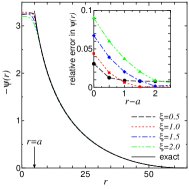
Figure 1: Electrostatic potential $\psi(r)$ around an infinitely long cylindrical rod of radius $a=5$ as a function of the distance from the center. The solid line indicates the analytic solution. The electrostatic potential and the length are measured in units of $k_{B}T/e$ and $\lambda_{B}$, respectively. Inset: relative error in the electrostatic potential for $\xi=0.5$ (circles), $1.0$ (squares), $1.5$ (diamonds), and $2.0$ (triangles) as a function of $r-a$.

To test the accuracy of the present method, we first consider a rod located at a center of the cylindrical (Wigner–Seitz) cell whose inner radius is $R=64$. Here we assume the system contains no additional salt. The analytical solution of the PB equation is known for this simple geometry, and the electrostatic potential is given by Fuoss et al. (1951); Alfrey et al. (1951)

$$\psi(r)=\ln\left[\frac{(\kappa_{D}r)^{2}}{R_{m}}\cos^{2}\left(\gamma\ln\left[\frac{r}{R_{m}}\right]\right)\right],$$ (18)

for $a<r<R$. Here, the constant $\gamma$ is determined as the solution of the algebraic equation

$$\tan^{-1}\left(\frac{\lambda-1}{\gamma}\right)+\tan^{-1}\left(\frac{1}{\gamma}\right)-\gamma\ln\left(\frac{R}{a}\right)=0,$$ (19)

where the constant $R_{m}$ is given by

$$R_{m}=R\exp\left[\frac{1}{\gamma}\tan^{-1}\left(\frac{\lambda-1}{\gamma}\right)\right].$$ (20)

Furthermore, the inverse screening length $\kappa_{D}$ is defined by $\kappa_{D}^{2}=4(1+\gamma^{2})/R$. The electrostatic potential is calculated using our method with $\xi=0.5$, $1.0$, $1.5$, and $2.0$ and plotted in Fig. 1. We see that the numerical results are in good agreements with the analytic solution for $r-a>\xi$, though some deviations are found for $r-a\leq\xi$ as an artifact of the smoothed profile. We emphasize that the inset of Fig. 1 shows the relative error $(\psi(r,\xi)-\psi_{\rm exact}(r))/\psi_{\rm exact}(r)$ is only within $1\%$ for $r-a>\xi$.

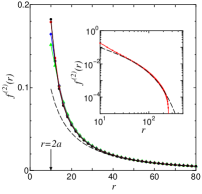
Figure 2: The pair force $f^{(2)}(r)$ between two colloidal disks as a function of the inter-disk separation $r$ with $\xi=0.5$ (circles), $1.0$ (squares), $1.5$ (diamonds), and $2.0$ (triangles). The dashed line indicates the LPB solution. The units of force and length are $k_{B}T/\lambda_{B}^{2}$ and $\lambda_{B}$, respectively. Inset: log-log plot of $f^{(2)}(r)$.

We next consider the pair interaction between charged disks immersed in a solution of counterions and coions. The system consists of $1024\times 1024$ grid points with the periodic boundary condition. The linear length of the system is $L=512$ and the Debye screening length is chosen as $\lambda_{D}=50$ in unit of $\lambda_{B}$. The equilibrium density profile is calculated for given inter-disk separations $r$, then, the force acting on the pair $f^{(2)}(r)$ is calculated using Eq. (16) for different values of the interface thickness $\xi=0.5$, $1.0$, $1.5$, and $2.0$. In Fig. 2, the force obtained by the present method is plotted and compared with the analytical solution of the linearized PB (LPB) equation Hansen and Löwen (2000), $f_{LPB}^{(2)}(r)=-dv/dr$ with

$$v(r)=\frac{(\lambda e)^{2}}{(\lambda_{D}^{-1}aK_{1}(a/\lambda_{D}))^{2}\epsilon}K_{0}(r/\lambda_{D}),$$ (21)

where $K_{0}(x)$ and $K_{1}(x)$ are Bessel functions of imaginary argument. Since the thickness of the electric double layer is roughly given by the Debye screening length $\lambda_{D}$, the force obtained by our numerical method agrees well with the linearized solution $f_{LPB}^{(2)}(r)$ for $r-2a>\lambda_{D}$. For short distances $r-2a<\lambda_{D}$, on the other hand, deviations from the LPB solution become notable. It is seen in the inset of Fig. 2 that the deviations between numerical results and the LPB solution become notable also for large $r$. This is nothing more than the artifact of the periodic boundary condition used in our numerical calculations where $f^{(2)}(r)$ must be zero at $r=L/2=256$.

The dependence of the interface thickness $\xi$ on $f^{(2)}(r)$ is similar to the case of he electrostatic potential $\psi(r)$ shown in Fig. 1. The all numerical curves in Fig. 2 are almost identical (within $1\%$ error) for $r-2a<2\xi$, while some deviations are observed for very short distances $r-2a\leq 2\xi$. In this case, the overlapping of the interface functions $\phi_{i}({\mbox{\boldmath$r$}})$ occurs between two disks. If we use a very small $\xi$ and an infinite number of grid points, we may reproduce the force curve obtained by more accurate, but numerically more expensive, methods like FEM quantitatively for small inter-disk separations. However, the numerical cost would also be very expensive in such a case. In other words, the trade-off for the increase in numerical efficiency using the non-zero interface thickness is some loss of the numerical accuracy. This may give rise to some quantitative errors when the separation between colloids are very small $r-2a\leq 2\xi$.

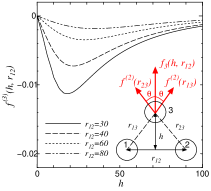
Figure 3: The three-body force $f^{(3)}(h,r_{12})$ acting on the third disk as a function of $h$ defined in the inset. Four curves are plotted for different values of $r_{12}$, the inter-disk separation of disks 1 and 2. The units of force and length are $k_{B}T/\lambda_{B}^{2}$ and $\lambda_{B}$, respectively.

Thirdly, we consider a system with three disks in order to examine three-body interactions acting on charged colloidal disks. Physical parameters were chosen identical to the two-disk case. The geometry of the three-disk system is shown in the inset of Fig. 3. The third disk is located in the mid-plane of the first and the second disks which have fixed separations $r_{12}$. We calculated the total force $f_{3}(h,r_{12})$ acting on the third disk with varying $h$, the distance from the axis connecting the first and second disks. Since $f_{3}(h,r_{12})$ is always vertical because of the symmetry, the vertical component of the three-body force $f^{(3)}(h,r_{12})$ acting on the third disk can be defined by

$$f^{(3)}(h,r_{12})\equiv f_{3}(h,r_{12})-f^{(2)}(r_{13})\cos\theta-f^{(2)}(r_{23})\cos\theta,$$ (22)

where $r_{ij}$ denotes the distance between the $i$th and $j$th disks, and $\theta$ is defined as $\cos\theta=h/r_{13}$. In Eq. (22), $r_{13}=r_{23}$ and $h=\sqrt{r_{13}^{2}-(r_{12}/2)^{2}}$ due to the symmetry of the geometry, and the pair force $f^{(2)}$ is given by the numerical results shown in Fig. 2. Figure 3 shows $f^{(3)}(h,r_{12})$ as a function of $h$ with four different values of $r_{12}$. Although we illustrate the numerical results only with $\xi=1.0$, we have carried out the same calculations also with $\xi=0.5$, $1.5$, and $2.0$. For the three-disk geometry examined here, all the curves tend to collapse onto each other within $1\%$ deviations. It is seen in Fig. 3 that the three-body force $f^{(3)}(h,r_{12})$ is always attractive in this geometry. This tendency agrees well with the results in Ref. Russ et al. (2002) where similar calculations have been performed by using FEM. A similar tendency has been observed in microscopic MD Löwen and Allahyarov (1998) and MC Wu et al. (2000) simulations as well as recent experiments Brunner et al. (2004); Dobnikar et al. (2004) for the same geometry in three-dimensional systems.

Figure 4: Configurations of colloidal disks in the initial (a) and the final (b) states. The temporal charge density $(1-\phi({\mbox{\boldmath$r$}}))e\rho_{c}^{eq}({\mbox{\boldmath$r$}})$ is shown with a color map. The scale of the color map is shown at the bottom in units of $e\lambda_{B}^{-3}$.

Finally, we performed a simple demonstration for the crystallization of $N=42$ colloidal disks interacting each other. Here, the system consists of $256\times 256$ grid points with the periodic boundary condition and the linear length of the system is $L=256$ while the other parameters are identical to those in the previous cases of $N=2$ and $3$. The positions of colloidal disks are followed by the steepest descent-type equation of motion

$$\zeta\frac{d{\mbox{\boldmath$R$}}_{i}}{dt}={\mbox{\boldmath$f$}}_{i}^{PP}+{\mbox{\boldmath$f$}}_{i}^{PS},$$ (23)

which is obtained by substituting $d^{2}{\mbox{\boldmath$R$}}_{i}/dt^{2}=0$, ${\mbox{\boldmath$f$}}_{i}^{R}=0$, and ${\mbox{\boldmath$f$}}_{i}^{H}=-\zeta d{\mbox{\boldmath$R$}}_{i}/dt$ with the friction constant $\zeta$ in Eq. (17). ${\mbox{\boldmath$f$}}_{i}^{PP}\equiv-\partial E_{PP}/\partial{\mbox{\boldmath$R$}}_{i}$ is the force arising from the potential $E_{PP}$ acting directly between a pair of colloidal disks. We defined $E_{PP}$ as the repulsive part of the Lennard–Jones potential, $E_{PP}/k_{B}T=0.4\sum_{i=1}^{N-1}\sum_{j=i+1}^{N}[(2a/|{\mbox{\boldmath$R$}}_{i}-{\mbox{\boldmath$R$}}_{j}|)^{12}-(2a/|{\mbox{\boldmath$R$}}_{i}-{\mbox{\boldmath$R$}}_{j}|)^{6}+1/4]$ truncated at the minimum distance $|{\mbox{\boldmath$R$}}_{i}-{\mbox{\boldmath$R$}}_{j}|=2^{7/6}a$. In Fig. 4, we show snapshots of the initial (a) and the final (b) configurations. Starting from a non-overlapping random configuration shown in Fig. 4(a), the colloidal disks move simply to reduce the total free energy. Eventually, the system attains a crystalline state with a hexagonal close packed structure shown in Fig. 4(b) even at a very small packing fraction $\eta\equiv\pi a^{2}N/L^{2}\simeq 0.05$ of colloid without any effective long-range interactions between colloidal disks. Similar crystalline structures have been observed in real experiments on charge-stabilized colloids Gast and Russel (1998). It is worth mentioning the computational efficiency of our numerical method. The demonstration shown in Fig 4, which required $600$ time steps, takes only one hour on a PC with a single Pentium4 2.8GHz CPU.

IV concluding remarks

A mesoscopic first-principle method are proposed for simulating charged colloidal dispersions. In order to remove the numerical inefficiency due to the moving boundary condition imposed on the colloid surface, a smoothed profile was introduced to represent the colloid-solvent interface. In our method, the effects of counterions are considered within the framework of a density functional theory. Furthermore, many-body effects among charged colloids are also included properly. We have examined the accuracy of the present method by changing the interface thickness $\xi$ and found that the accuracy is satisfactory as far as the distance between colloidal disks is larger than $2(a+\xi)$.

Our final goal is to develop a simulation method applicable to dynamical problems of charged colloidal dispersions such as electrophoresis where the coupling between hydrodynamics and electrostatic interactions are crucial Russel et al. (1989). In the present paper, we restricted our attentions only to static problems with employing the adiabatic approximation, i.e., $\rho_{\pm}({\mbox{\boldmath$r$}})$ follows instantaneously to the motions of the colloidal disks or particles. This is OK for calculating stable colloidal structures in the dispersions. In the cases of dynamical problems, the time evolution of $\rho_{\pm}({\mbox{\boldmath$r$}})$ should be determined by coupling equations of hydrodynamics and thermal diffusion. The PB equation is not appropriate for treating dynamical problems in which the counterion density becomes anisotropic around a particle because of the friction between counterions and solvents. Dipoles are induced if this happens, and thus interactions between colloids are no longer screened. There appear long-range interactions between colloids, which must be important in many practical problems including electrophoresis for example. Integration of the present method and the method for colloids in Newtonian fluids Nakayama and Yamamoto (2004) present promising approaches to solve these cases, and efforts to this end are currently underway.

As this paper was being written for publication, we became aware of a parallel effort by Kodama et al. Kodama et al. (2004). While the omission of several details in their implementation make a detailed comparison between the two approaches impossible at this time, it will be most useful in the future to make a detailed comparison of the two methods both on efficiency and accuracy.