Neighborhood models of minority opinion spreading

Abstract

We study the effect of finite size population in Galam’s model [Eur. Phys. J. B 25 (2002) 403] of minority opinion spreading and introduce neighborhood models that account for local spatial effects. For systems of different sizes $N$, the time to reach consensus is shown to scale as $\ln N$ in the original version, while the evolution is much slower in the new neighborhood models. The threshold value of the initial concentration of minority supporters for the defeat of the initial majority, which is independent of $N$ in Galam’s model, goes to zero with growing system size in the neighborhood models. This is a consequence of the existence of a critical size for the growth of a local domain of minority supporters.

I Introduction

There is a growing interest among theoretical physicists in complex phenomena in fields departing from the traditional realm of physics research. In particular, the application of statistical physics methods to social phenomena is discussed in several reviews weidlich ; Ball ; stauffer04 ; Gal04 . One of the sociological problems that attracts much attention is the building or the lack of consensus out of some initial condition. There are several different models that simulate and analyze the dynamics of such processes in opinion formation, cultural dynamics, etc. Gal03 ; Gal00 ; Gal01 ; Gal02 ; complex1 ; heg01 ; sznajd01 ; sznajd02 ; stauffer1 ; stauffer11 ; stauffer2 ; Castellano ; Klemm1 ; Klemm2 ; Klemm3 ; krapi01 ; Mobilia1 ; Mobilia2 . Among all those models, the one introduced by Galam Gal01 ; Gal02 to describe the spreading of a minority opinion, incorporates basic mechanisms of social inertia, resulting in democratic rejection of social reforms initially favored by a majority. In this model, individuals gather during their social life in meeting cells of different sizes where they discuss about a topic until a final decision, in favor or against, is taken by the entire group. The decision is based on the majority rule such that everybody in the meeting cell adopts the opinion of the majority. Galam introduced the idea of “social inertia” in the form of a bias corresponding to a resistance to changes or reforms, that is: in case of tie, one of the decisions (in the original version, the one against) is systematically adopted. We will describe in detail the model and its main conclusions in the next sections. This simple model is able to explain why an initially minority opinion can become a majority in the long run. An interesting example was its application to the spread of rumors concerning some September 11-th opinions in France Gal02 . One of the major conclusions of the mean-field-like analysis in Ref.Gal01 , is the existence of a threshold value $p_{c}<1/2$ for the initial concentration of individuals with the minority opinion (against the social reform). For $p>p_{c}$ every individual eventually adopts the opinion of the initial minority, so that the social reform is rejected and the status quo is maintained. A related message of this result is that a rumor spreads, although initially supported by a minority, if the society has some bias towards accepting it.

Galam traces back his results to dynamical effects produced by the existence of asymmetric unstable points previously considered by Granovetter Granovetter and Schelling Schelling . These are fixed points of recursion relations describing the dynamics of the fraction of a population adopting one of two possible choices. In threshold models these relations are obtained considering a mean field type of interaction in which individual thresholds to change choice (tolerance) are compared with the fraction of the population that has already adopted the new choice. Granovetter himself Granovetter discusses that the stability of the fixed points can be changed by spatial effects, noting that the assumption that each individual is responsive to the behavior of all the others is often inappropriate. In Gal01 such complete connectedness of the population seems to be circumvented by the introduction of the meeting cells. Only individuals in each meeting cell interact among themselves. In this sense each meeting cell plays the role of a bounded neighborhood Schelling and it is still possible to obtain analytically recursion relations for the dynamics. However, contrary to the bounded neighborhood model of Schelling, individuals enter and leave these neighborhoods randomly, and the neighborhoods do not have any characteristic identity other than their sizes. Even if the meeting cells are thought of as sites where local discussions take place, Galam’s model Gal01 does not incorporate local interactions since the individuals are randomly redistributed in the meeting cells at each time step of the dynamics.

The alternative considered by Schelling to the bounded neighborhood model is a spatial proximity model in which everybody defines his neighborhood by reference to his own spatial location. The spatial arrangement or configuration within the neighborhood mediates the interactions. We propose here a different neighborhood model which shares some characteristics with the bounded neighborhood and spatial proximity models: The meeting cells are neighborhoods defined by spatial location, therefore introducing important local effects, but the interaction within the neighborhood is independent of the spatial configuration within the cell. Contrary to the model in Gal01 the individuals are here located at fixed sites of a lattice. The local neighborhood or meeting cell in which a given individual interacts changes with time, reflecting neighborhoods of changing shape and size. Such neighborhood model could be appropriate for a relatively primitive society in which interactions are predominantly among neighbors, but the size of the neighborhood or interaction range is not fixed.

A different version of Galam’s model was introduced by Stauffer stauffer11 . At variance with our neighborhood models in which individuals are fixed in the sites of a lattice and the meeting cells have a maximum size, Stauffer considers the situation in which individuals freely diffuse in a lattice with only a fraction of sites being occupied. This diffusion process leads to the formation of “natural” clusters which play the role of our meeting cells: It is within each one of these clusters in which the rule of majority opinion and bias towards minority in case of a tie are taken. Stauffer finds in his model that the time to reach a consensus opinion grows logarithmically with system size $N$. We also find this dependence in the original model of Galam, while in our neighborhood models the consensus time takes much larger values and is compatible with a power law dependence. A related model, including the figure of the “contrarians” (that is, people that always oppose to the majority position), was later introduced by Galam Gal04b and also analyzed by Stauffer stauffer4 .

A main consequence of introducing the spatial effects considered in our neighborhood models is that the threshold found in Gal01 disappears with system size, i.e. $\lim_{N\to\infty}p_{c}=0$, so that in large systems the minority opinion always spreads and overcomes the initial majority for whatever initial proportion of the minority opinion. This is a consequence of the existence of a critical size for a local domain of minority supporters. Domains of size larger than the critical one will expand and occupy the whole system. For large systems there is always a finite probability to have a domain of over-critical size in the initial condition. While in traditional Statistical Physics we are mostly concerned with the thermodynamic limit of large systems, these findings emphasize the important role of system size in the sociological context of models of interacting individual entities.

The outline of the paper is as follows. Section 2 reviews the original definition of Galam’s model Gal01 ; Gal02 and introduces our new local neighborhood models. In Sect. 3 we go beyond the mean field limit of Refs.Gal01 ; Gal02 by discussing the system size dependence of the predictions of the original model. Steady-state and dynamical properties of our neighborhood models are presented in Sects. 4 and 5. General conclusions are summarized in Sect. 6.

II Definition of the model

II.1 Galam’s original non-local model

The model considers a population of $N$ individuals who randomly gather in “meeting cells”. A meeting cell is just defined by the number of individuals $k$ that can meet in the cell. Let us define $a_{k}$ as the probability that a particular person is found in a cell of size $k$. Obviously, it is $\sum_{k}a_{k}=1$.

The dynamics of the model is as follows: first the meeting cells are defined by giving each one a size according to the probability distribution $\{a_{k}\}$, such that the sum of all the cell sizes equals the number of individuals $N$, but otherwise their location or shape are not specified. These cells are not modified during the whole dynamical process. The persons have an initial binary (against, $+$, or in favor, $-$) opinion about a certain topic. The probability that a person shares the $+$ opinion at time $t$ is $P_{+}(t)$ and an equivalent definition for $P_{-}(t)=1-P_{+}(t)$. Initially one sets $P_{+}(t=0)=p$. Alternatively, $P_{+}(t)$ can be thought of as the proportion of people supporting opinion $+$ at time $t$.

The $N$ individuals are then distributed randomly among the different cells. The basic premise of the model is that all the people within a cell adopt the opinion of the majority of the cell. Furthermore, in the case of a tie (which can only occur if the cell size $k$ is an even number), one of the opinions, that we arbitrarily identify with the $+$ opinion, is adopted. Once an opinion within the different cells has been taken, time increases by one, $t\to t+1$ and the individuals rearrange by distributing themselves again randomly among the different cells.

The main finding of this model is that an initially minority opinion, corresponding to $p<1/2$ can win in the long term. This is an effect of the tie rule that selects the $+$ opinion in case of a tie.

It is possible to write down a recursion relation for the density of people that at time $t$ have the $+$ opinion as Gal01

$$P_{+}(t+1)=\sum_{k=1}^{M}a_{k}\,\sum_{j=\left[\frac{M}{2}+1\right]}^{M}{k\choose j}P_{+}(t)^{j}\,\left[1-P_{+}(t)\right]^{k-j},$$ (1)

Simultaneously

$$P_{-}(t+1)=\sum_{k=1}^{M}a_{k}\,\sum_{j=\left[\frac{M+1}{2}\right]}^{M}{k\choose j}P_{-}(t)^{j}\,\left[1-P_{-}(t)\right]^{k-j},$$ (2)

the notation $[x]$ indicates the integer part of $x$. This is a mean-field equation that neglects possible fluctuations.

For a wide range of distributions $\{a_{k}\}$ this map has three fixed points: two stable ones at $P_{+}=1$ and $P_{+}=0$ and an unstable one, the faith point, at $P_{+}=p_{c}$. Hence, the dynamics is such that

$$\lim_{t\to\infty}P_{+}(t)=\left\{\begin{array}[]{lr}1&\hbox{if }\qquad P_{+}(0)>p_{c}\\ 0&\hbox{if }\qquad P_{+}(0)<p_{c}\end{array}\right.$$ (3)

II.2 Neighborhood models

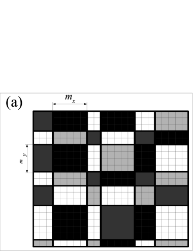
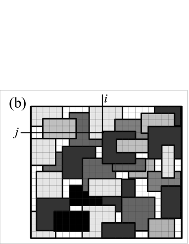
Figure 1: (a) Regular 2D tessellation: All the cells are simultaneously created, being $m_{x}$ and $m_{y}$ uniformly distributed between 1 and $M$. (b) Locally grown tessellation: A site ($i,j$) is chosen, and from it a cell of size $m_{x},m_{y}$, excluding those already belonging to other cell.

We now introduce our Neighborhood Models that incorporate local spatial effects in the interacting dynamics proposed by Galam. In these local models, individuals are fixed at the sites of a regular lattice and they interact with other individuals in their spatial neighborhood. We have considered several cases:

II.2.1 One-dimensional neighborhood model: synchronous update

The $N$ individuals are distributed at the sites of a linear lattice $i=1,2,\dots,N$. Once distributed, they never move again. Initially they are assigned a probability $p$ of adopting the $+$ opinion, and $(1-p)$ the $-$ opinion. The dynamics starts by defining the meeting cells $k=1,2,\dots$ as the segments $[i_{k},i_{k+1}-1]$ of length $m_{k}=i_{k+1}-i_{k}$. The cell sizes $m_{k}$ are distributed according to a uniform distribution in the interval $[1,M]$. The average cell size is hence $\langle m_{k}\rangle=\frac{(M+1)}{2}$ and the average number of cells is $N/\langle m_{k}\rangle$. Once the cells are defined, the dynamical rules of Galam’s model are applied synchronously to all the cells, time increases by one $t\to t+1$. In the next time step, new cells, uncorrelated to the previous ones are defined and the dynamical rules applied again. The process continues until there is a single common opinion in the whole system.

II.2.2 Two-dimensional neighborhood model: synchronous update

The two-dimensional case is very similar to the 1D version explained above. The only difference is the way the meeting cells are defined in the two-dimensional lattice. An individual is now characterized by two indexes $(i,j)$ with $1\leq i,j\leq L$, such that the total number of individuals is $N=L^{2}$. We have considered two different definitions of the cells originated in two tessellations of the plane: (a) the regular tessellation and (b) the locally-grown tessellation. In the regular tessellation, we define segments in the $i$ and $j$ axis independently, such that the sizes are in both cases uniformly distributed between $1$ and $M$ in the same way that we did in the one-dimensional case. Figure 1a plots a typical example. In the locally-grown tessellation we first choose a site of the lattice and then define a rectangle around it whose sides are both uniformly distributed between $1$ and $M$. The cell is defined then as the sites in the resulting rectangle excluding those sites that already were part of a previously defined cell. Figure 1b shows a typical example.

Once the cells are defined, the dynamical rules are applied synchronously to all the cells and a common opinion is formed within each cell. Time then increases by one $t\to t+1$. In the next time step, new cells are defined and the process continues until a consensus opinion is reached in the whole population.

II.2.3 Asynchronous update

The 1D and 2D models have been also considered in the asynchronous update version. In this case, a lattice site is randomly chosen and a cell defined around it as a segment (1D) of size $m$ or a rectangle (2D) of size $(m_{x},m_{y})$. It is only within this cell that the biased majority rule is applied. Time increases by $t\to t+m/N$ in 1D and by $t\to t+(m_{x}\,m_{y})/N$ in 2D. Then a new site is selected randomly and the process iterates until a consensus opinion is obtained.

III Results for Galam’s original non-local model.

We present in this section an analysis of Galam’s original non-local model. Our aim is to go beyond the mean-field approach of references Gal01 ; Gal02 ; Gal04b by studying the system size dependence of the different magnitudes of interest. Some of the results are based on numerical simulations of the model.

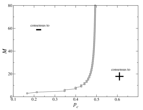
Figure 2: Phase diagram of the original Galam’s model in the plane ($p_{c}$, $M$).

We consider $N$ individuals that distribute themselves randomly in meeting cells whose size is uniformly distributed between $1$ and $M$. In the notation of Eq. (1), this means that $a_{k}=2k/(M(M+1))$, $k\in[1,M]$, as it follows from the fact that $a_{k}$ measures the probability for an individual of being in any of the $k$ sites of a cell of size $k$. Initially we assign to each of the persons any of the two possible opinions, such that the probability of having the favored opinion is $p$. Again, in the language of Eq. (1), we are setting $P_{+}(0)=p$. We then apply the dynamical rules of Galam’s model until a consensus opinion is formed. By iteration of this procedure, we measure the probability $\rho$ that the consensus opinion coincides with the favored one, $+$. This is precisely defined as the fraction of realizations that end up in the favored $+$ opinion.

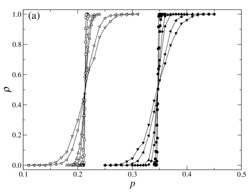
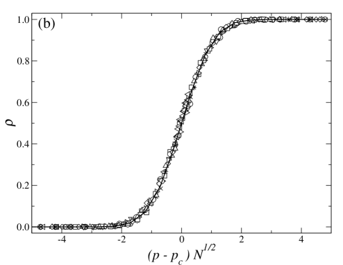
Figure 3: (a) Order parameter in Galam’s non-local model. The white symbols correspond to the case $M=4$ ($p_{c}=0.2133077908\dots$), while the black ones to $M=5$ ($p_{c}=0.3467871056\dots$). The values of $N$ range between $N=10^{3}$ and $N=10^{6}$. (b) The order parameter for both values of $M$ for rescaled values of $p$ according to $(p-p_{c})N^{1/2}$. Also, it is shown a fit with the function $\rho(p,N)=(1+\hbox{erf}(x/1.17))/2$ with the scaling variable $x=(p-p_{c})/N^{1/2}$.

The analysis of Eq. (1) predicts a first order phase transition in the sense that the “order parameter” $\rho=0$ if $p<p_{c}$ and $\rho=1$ if $p>p_{c}$. In Fig. 2 we show, in the parameter space $(p_{c},M)$, the regions where the two solutions, as obtained by finding numerically the non-trivial fixed point of the recurrence Eq. (1), exists. Note that, as expected, the larger the decision cells, the closer the faith point to $1/2$. Notice also in this figure that some pairs of consecutive values of $M$ give almost the same value for $p_{c}$. The reason is that, for odd values of $M$, the rule that applies in case of a tie is used only up to the value $M-1$ (which is even), so odd numbers give similar values of $p_{c}$ than the precedent even number.

Since Eq. (1) neglects possible system size fluctuations, Eq. (3) this result is only valid in the limit $N\to\infty$. We plot in Fig. 3a the raw results of our simulations for different system sizes. The analysis carried out in Fig. 3b shows that the asymptotic results of $N\to\infty$ are achieved by means of the following scaling relation

$$\rho(p,N)=f\left((p-p_{c})\,N^{-1/2}\right).$$ (4)

Therefore, there is a region of size $N^{-1/2}$ where there is a significant probability that the results differ from the infinite size limit.

We now analyze the time $T$ it takes to reach the consensus opinion. Strictly speaking, in the mean field approach the number of iterations needed for Eq. (1) to converge to the fixed point is infinity. In Ref. Gal01 it was adopted the criterion that the fixed point had been reached at the time $T$ such that $P_{+}(T)$ differs from the fixed point in less that $0.01$. In our simulations, and as in reference stauffer11 , it is natural to define the time $T$ as the finite number of steps needed to reach the consensus opinion. We plot in Fig. 4 the time $T$ as a function of the initial probability $p$ of the favored opinion. It can be seen that the time $T$ increases with increasing system size and takes its maximum value at the faith point. A closer analysis shown in figure 5 shows that, for all values of $p$, the time needed to reach the consensus increases logarithmically with $N$. It is interesting to note that the same logarithmic dependence was found in Ref. stauffer11 for the model accounting for Brownian diffusion.

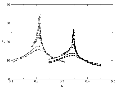
Figure 4: Time that it takes to the system to reach the consensus state as a function of the initial probability $p$ for different system sizes. The white symbols correspond to the case $M=4$ while the black ones to $M=5$. The values of $N$ range between $N=10^{3}$ and $N=10^{6}$.

Figure 5: Time to reach the consensus state as a function of system size for different values of $p$ and $M=4$. Two different slopes can be seen for values of $p$ greater and lower than the critical value $p_{c}\sim 0.21$. Also the predicted slopes are plotted.

A simple argument can help to understand this logarithmic behavior. One can mimic the size dependence of the time $T$ by noticing that the definition used in the numerical simulations is equivalent to define $T$ as the value for which $P_{+}(T)={\mathcal{O}}(1/N)$ or $1-P_{+}(T)={\mathcal{O}}(1/N)$, since $1/N$ is the minimum possible value for $p$ over $p=0$. This can be now obtained by linearizing the evolution equation around any of the fixed points $0,1$. Defining respectively $\delta(t)=P_{+}(t)-0$ or $\delta(t)=P_{+}(t)-1$, and replacing in the evolution equation (1) $P_{+}(t+1)\equiv F[P_{+}(t)]$, we obtain at first order:

$$\delta(t+1)=\lambda\,\delta(t),$$ (5)

where $\lambda\equiv F^{\prime}[0]$ and $\lambda\equiv F^{\prime}[1]$, respectively. In this linear regime, we have simply: $\delta(t)=\lambda^{t}\,\delta(0)$ and according to the definition above,

$$T\sim\frac{\ln\delta(0)-\ln N}{\ln\lambda},$$ (6)

where the correct value of $\lambda$ has to be used in each case. This is the logarithmic behavior observed in the simulations. Furthermore, the slope of the logarithmic law will depend on the fixed point at which the system tends. So, at one side of the critical point, the slope should be different than at the other. Figure 5 shows the confirmation of this prediction, where it is seen that for high values of $p$ (above the faith point) the slope is quite different than for lower values. For $M=4$, the predicted values for $\lambda$ are $\lambda=1/10$ and $\lambda=1/2$ for the fixed point at $P_{+}=1$ and $P_{+}=0$ respectively. The corresponding slopes, $-1/\ln\lambda$, are $0.434\dots$ and $1.442\dots$. As shown in the figure, these values agree well with the measured slopes. The only discrepancy is for $p\approx p_{c}$ for which the time needed to reach consensus must include as well the time needed to leave the fixed point $p_{c}$.

IV Neighborhood models: steady state properties

In this section we consider the steady state properties of our neighborhood models defined in Sect. II.2. We will see that the introduction of spatial local effects leads to a very different behavior than for the non-local version of the previous section in which individuals were distributed randomly in fixed cells.

In our neighborhood versions, similarly to the original Galam model, it turns out that a consensus opinion is always reached in a finite number of steps. We first consider the order parameter, $\rho$, defined as the probability that the consensus opinion coincides with the favored one. Figures 6 and 7 show that, both in the 1D and the 2D cases, the order parameter $\rho$ is an increasing function of the initial probability $p$ of adopting the favored opinion. It is possible to define, quite arbitrarily, the transition point $p_{c}$ as the one for which $\rho=1/2$. However, $p_{c}$ depends upon the system size as a power law $p_{c}(N)\sim N^{-\alpha}$, hence for increasing $N$ the transition point tends to $p_{c}=0$. In other words, the transition disappears in the thermodynamic limit, $N\to\infty$, and the favored opinion, in that limit, is always the selected one independently of the initial choice. More precisely, the data can be described by the scaling law

$$\rho(p,N)=\rho(pN^{\alpha}).$$ (7)

The exponent $\alpha$ depends on the dimension and on the maximum size $M$ of the domains. In Fig. 8 we plot the $M$-dependence of $\alpha$ in several 1D and 2D neighborhood models. Notice that $\alpha$ decreases for increasing $M$ and it depends on the system dimension, but it is basically independent of the local rules defined. Alternatively, for fixed $p$ we can define a critical value $N_{c}(p)$ such that a small population $N<N_{c}(p)$ tends not to propagate the initially minority opinion.

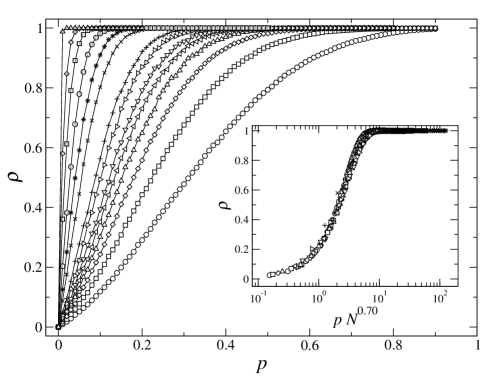
Figure 6: Order parameter for the neighborhood one-dimensional system with synchronous update for $M=5$. The system size ranges between $N=10$ (rightmost curve) and $N=10^{4}$ (leftmost curve). The inset shows the validity of the scaling law $\rho=\rho(pN^{\alpha})$ with $\alpha=0.7$.

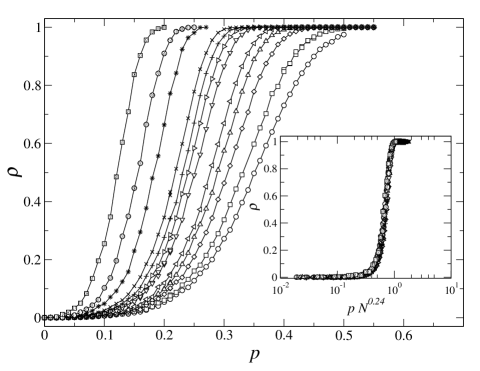
Figure 7: Same as Fig. 6 for neighborhood models with synchronous update and regular 2D tessellation. $M=5$. The system size is $N=L\times L$ with $L$ between $L=15$ (rightmost curve) and $L=10^{3}$ (leftmost curve). The inset shows the scaling law with $\alpha=0.24$.

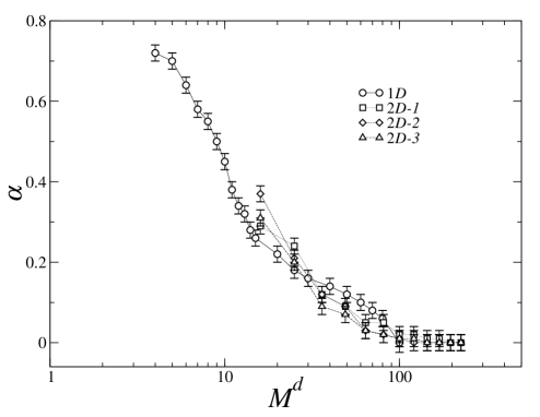
Figure 8: Scaling exponent defined in equation (7) as a function of $M^{d}$. The different curves correspond to: 1D (one-dimensional system, synchronous update), while the bi-dimensional are: 2D-1 (synchronous update, regular tessellation), 2D-2 (synchronous update, locally grown tessellation), 2D-3 (asynchronous update).

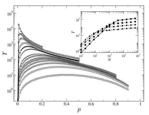
Figure 9: Time to reach the consensus vs $p$, for synchronous 1D local cells and for $M=5$. Same symbols and systems sizes than in Fig. 6. The inset shows the time to reach consensus plotted against system size, for different values of $p$, i.e. $p=0.2$ (triangles), $p=0.1$ (diamonds), $p=0.05$ (circles), $p=0.02$ (squares). Two power-laws are observed (depending on whether $N<N_{c}(p)$ or $N>N_{c}(p)$); for $N<N_{c}$, $\beta\approx 1.6$ and in the regime $N>N_{c}(p)$, $\beta\approx 0.2$.

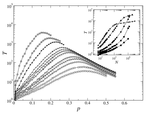
Figure 10: Time to reach the final consensus state vs $p$, for the $2D$ cells, and for $M=5$. Same symbols and systems sizes than in Fig. 7. The inset shows the time to reach consensus for fixed values of $p$: $p=0.3$ (stars), $p=0.2$ (triangles), $p=0.1$ (diamonds), $p=0.05$ (circles), $p=0.02$ (squares). The results are quite similar to those depicted in Figure 9. In this case, for $N<N_{c}(p)$, $\beta\approx 0.6$ and in the regime $N>N_{c}(p)$ (a regime only clearly seen in the cases $p=0.3,0.2$), $\beta\approx 0.1$.

V Neighborhood models: dynamical evolution

There are several differences between the evolution in the neighborhood and non-local models. We first analyze the time $T$ needed to reach the consensus. As in Galam’s original model, the data in Figs. 9 and 10 for the 1D and 2D cases, respectively, show that for fixed $N$, the time $T$ reaches a maximum at the critical point $p_{c}(N)$. Notice that the numerical values for $T$ are much larger in the local models that they were in the original model. Furthermore, as shown in the insets of Figs. 9 and 10, for fixed $p$, the time $T$ has two different growth laws according to whether the population $N$ is smaller or larger than the critical size $N_{c}(p)$. For $N<N_{c}(p)$ the time $T$ increases as a power-law $T\sim N^{\beta}$ of the system size $N$ with $\beta=1.6(0.6)$ for $d=1(2)$. For $N>N_{c}(p)$ the data are compatible with a power law with smaller exponents, although it can not be completely excluded a logarithmic dependence in this case.

In Fig. 11 we plot several snapshots corresponding to the evolution according to Galam’s original rules. It is seen that the evolution is very fast and at each time step the number of people favoring a particular opinion increases but due to the non-locality of the rules, one can not see any structured pattern of growth.

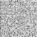
Figure 11: Plot of the dynamical evolution of a non-local system updated according to the synchronous update. Each frame correspond to a time, increasing from left to right and top to bottom. The system size is $N=256^{2}$ and $M=5$.

When using the neighborhood rules, however, it can be seen that, after a very short transient in which domains are formed, the ulterior evolution is by modification of the interfaces between the two possible types of domains.

Figure 12 depicts the dynamical evolution of the synchronous 1D version of the neighborhood model. It shows a linear growth of the size of domains of favored opinion. It is easy to predict the slope of the linear growth according to the following reasoning: the only evolution is produced if the discussion cell intercepts two domains with different opinions. Let us consider the position of an interface at time $t=0$. For cells of odd size, the bias rule does not apply and the interface does not move in the average. For cells of even size, the bias rule acts only in one case and it is easy to show that the location of the interface, on the average, increases by $1/2$. Therefore, the size of the domain of the favored opinion increase as $t/2$. Averaging for an equiprobability of having cells of size between 1 an $M$, yields a linear growth $\beta t$ with

$$\beta=2\frac{\left[\frac{M}{2}\right]\left[\frac{M}{2}+1\right]}{M(M+1)},$$ (8)

where $[x]$ once again denotes the integer part of $x$. The validity of this result for $M=5$ is shown in Fig. 12.

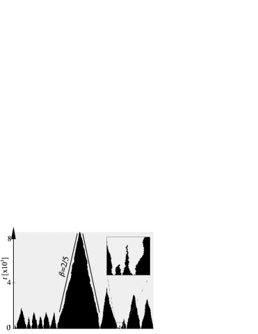
Figure 12: Plot of the dynamical evolution of a local 1D system. Each row corresponds to a time, increasing from bottom to top. The system size is $N=5000$ and $M=5$. It is also shown the predicted slope given by Eq. (8) The inset amplifies a small region for a short time evolution.

The 2D snapshots of the dynamical evolution, see Fig. 13, show that as in the 1D version, domains are formed in an initial transient, and after this, grow by interface dynamics. To characterize the growth of the characteristic size of the domains we calculate a characteristic radius $R_{c}$ defined as

$$R_{c}^{2}=\frac{\sum_{i}\delta_{+}(i)\vec{r_{i}}^{2}}{\sum_{i}\delta_{+}(i)}-\left(\frac{\sum_{i}\delta_{+}(i)\vec{r_{i}}}{\sum_{i}\delta_{+}(i)}\right)^{2}.$$ (9)

Where $\delta_{+}(i)$ is $1$ if individual $i$ supports opinion $+$, $0$ otherwise and $\vec{r_{i}}$ is the position in the square lattice of $i-$th individual. Figure 14 shows that this characteristic linear dimension grows linearly with time as in the 1D model.

The growth of domains in 1D and 2D occurs for those domains whose initial characteristic size is larger than a critical one $R^{*}$. When the initial size is larger than $R^{*}$, domains grow until they take over the whole system, while smaller domains shrink toward extinction. The quantitative calculation of the critical radius starts by placing a unique circular island of radius $r$ of minority people surrounded by the majority and watching it grow or shrink. This initial condition is quite different of that of a random initial distribution. In order to avoid finite size effects, one has to be careful to choose a system size $N$ such that the initial density $p=\pi r^{2}/N$ is lower than the critical one, $p_{c}$. In the inset of Fig. 15 we show that $\rho(r)$, the probability that an initial circle of radius $r$ grows, is indeed independent of system size. We define the critical radius as the value of $r$ such that $\rho(r)=0.5$. Figure 15 shows that the value of the critical radius increases linearly with $M$, both in 1D and in 2D models.

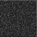
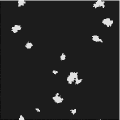
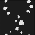
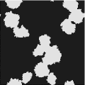
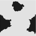
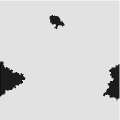
Figure 13: The dynamical evolution of a 2D local model updated according to the asynchronous rule is shown. In the simulation $N=400\times 400$, $M=5$ and $p=0.2$. The time increases from left to right and from top to bottom. The snapshots correspond, respectively to $T=0$, $20$, $52$, $106$, $276$, $394$, $594$ and $818$.

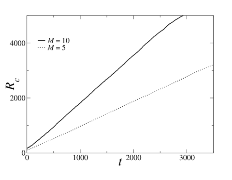
Figure 14: Characteristic radius, $R_{c}$ averaged over 100 independent runs as a function of time for a two-dimensional system updated according to the synchronous update and regular tessellation. $R_{c}$ is shown to grow linearly with time for different values of $M$. The initial condition is taken as a single circular domain of minority supporters with a radius $R>R^{*}$.

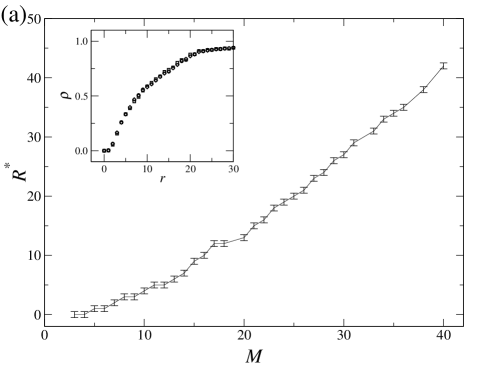
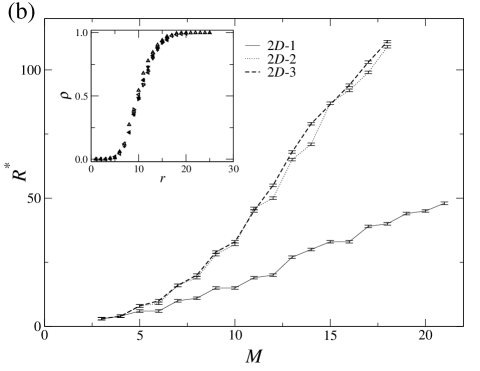
Figure 15: Critical radius vs $M$, for the different versions of the neighborhood systems: (a) 1D model. (b) 2D-1, 2D-2, 2D-3 as defined in Fig. 8. The insets show the probability $\rho(r)$ that an initial domain of radius $r$ grows; (a) corresponds to $M=15$ and (b) is for the 2D-1 model for $M=7$, both for different system sizes.

VI General conclusions

We have revisited Galam’s model Gal01 ; Gal02 of minority opinion spreading and introduced related neighborhood models that incorporate spatial local effects in the interactions. These models share basic characteristics with the bounded neighborhood and spatial proximity models of Schelling Schelling . In both cases we have considered in detail the role of system size in the properties of the system. For the original nonlocal version Gal01 ; Gal02 , we have found that the transition from initial minority final dominance to initial minority disappearance is smeared out in a region of size $N^{-1/2}$, while the time it takes to reach complete consensus increases as $\ln N$, as in Stauffer’s percolation model stauffer11 .

In our local neighborhood models, we have considered 1D and 2D lattices with regular and locally grown tessellations, both with synchronous and asynchronous updates. All these local versions behave qualitatively in the same way. The most important finding is that the threshold value for the initial minority concentration $p_{c}$ decreases as $N^{-\alpha}$, such that the transition from initial minority spreading to majority dominance disappears in the thermodynamic limit $N\to\infty$. The neighborhood models are, in this sense, more efficient to spread an initially minority opinion. However, while a nonlocal model is very fast in spreading a rumor, the corresponding relaxation times to reach consensus in the neighborhood models are much larger since they turn out to increase with a power of the system size $N$.

We have also shown that the fact that $lim_{N\to\infty}p_{c}=0$ is due to the existence of a critical size for a spatial domain of minority supporters. For large enough systems there is always an over-critical domain that spreads and occupies the whole system, with a characteristic average radius growing linearly with time. This critical size domain has some analogies with the critical nucleus of nucleation theory Gunton83 , but it has different characteristics. In classical nucleation the existence of a critical radius is due to the competition between surface tension and different bulk energy between the two possible homogeneous states. The concept of critical nucleus in this context is not meaningful for one-dimensional systems for which no surface tension exists. An over-critical droplet appears as a rare fluctuation in the bulk of a metastable state and it then grows deterministically. Noisy perturbations in the growth dynamics are generally a second order effect. In our case over-critical domains appear in the random initial condition. The critical size is here an average concept resulting from the competition of the bias favoring the minority opinion in case of a tie (analog of bulk energy difference) and a stochastic dynamics that might lead to the disappearance of the minority domain, surface tension being a second order effect. Critical size means here equal probability for the domain to spread or to collapse.

The existence of this critical size clearly shows an important difference between typical statistical physics problems and sociophysical ones. In the former case, one is mostly concerned with the thermodynamic limit of large systems, while these findings emphasize the important role of system size in the latter case.

Acknowledgments We thank P.Colet, V. M. Eguíluz and E. Hernández–García for fruitful discussions. We acknowledge financial support from MCYT (Spain) and FEDER through the projects BFM2001-0341-C02-01 and BFM2000-1108. HSW acknowledges partial support from ANPCyT, Argentine, and thanks the MECyD, Spain, for an award within the Sabbatical Program for Visiting Professors, and to the Universitat de les Illes Balears for the kind hospitality extended to him.

References

- (1) W. Weidlich, Sociodynamics-A systematic approach to mathematical modeling in social sciences (Taylor & Francis, London, 2002).
- (2) P. Ball, Utopia theory, Physics World (October 2003).
- (3) D. Stauffer, Introduction to Statistical Physics outside Physics, Physica A336, 1 (2004).
- (4) S. Galam, Sociophysics: a personal testimony, Physica A336, 49 (2004).
- (5) S. Galam, B. Chopard, A. Masselot and M. Droz, Eur. Phys. J. B 4 (1998) 529-531.
- (6) S. Galam and J. D. Zucker, Physica A 287 (2000) 644-659.
- (7) S. Galam, Eur. Phys. J. B 25 (2002) 403.
- (8) S. Galam, Physica A 320 (2003) 571-580.
- (9) G. Deffuant, D. Neau, F. Amblard and G. Weisbuch, Adv. Complex Syst. (2000) 3, 87; G. Weisbuch, G. Deffuant, F. Amblard and J.-P. Nadal, Complexity (2002) 7, 55.
- (10) R. Hegselmann and U. Krausse, J. of Artif. Soc. and Social Sim. 5 (2002) 3, http://www.soc.surrey.ac.uk/JASS/5/3/2.html
- (11) K. Sznajd-Weron and J. Sznajd, Int. J. Mod. Phys. C11 (2000) 1157; K. Sznajd-Weron, Phys. Rev. E 66 (2002) 046131; K. Sznajd-Weron and J. Sznajd, Int. J. Mod. Phys. C13 (2000) 115.
- (12) F. Slanina and H. Lavicka, Eur. Phys. J. B 35 (2003) 279.
- (13) D. Stauffer, A.O. Souza and S. Moss de Oliveira, Int. J. Mod. Phys. C11 (2000) 1239; D. Stauffer, Int. J. Mod. Phys. C13 (2002) 315; D. Stauffer and P. C. M. Oliveira, Eur. Phys. J. B 30 (2002) 587.
- (14) D.Stauffer, Int. J. Mod. Phys. C13 (2002) 975.
- (15) D. Stauffer, J. of Artificial Societies and Social Simulation 5 (2001) 1, http://www.soc.surrey.ac.uk/JASS/5/1/4.html; D. Stauffer, How to convince others?: Monte Carlo simulations of the Sznajd model, in Proc. Conf. on the Monte Carlo Method in the Physical Sciences, J.E. Gubernatis, Ed., (AIP, in press), cond-mat/0307133; D. Stauffer, Computing in Science and Engineering 5 (2003) 71.
- (16) C. Castellano, M. Marsili, and A. Vespignani, Phys. Rev. Lett. 85 (2000) 3536; D. Vilone, A. Vespignani and C. Castellano, Eur. Phys. J. B 30 (2002) 399.
- (17) K. Klemm, V. M. Eguiluz, R. Toral and M. San Miguel, Phys. Rev. E 67 (2003) 026120.
- (18) K. Klemm, V. M. Eguiluz, R. Toral and M. San Miguel, Phys. Rev. E 67 (2003) 045101R.
- (19) K. Klemm, V. M. Eguiluz, R. Toral and M. San Miguel, Globalization, polarization and cultural drift J. Economic Dynamics and Control (in press).
- (20) P.L. Krapivsky and S. Redner, Phys. Rev. Lett. 90 (2003) 238701.
- (21) M. Mobilia, Phys. Rev. Lett. 91 (2003) 028701.
- (22) M. Mobilia and S. Redner, cond-mat/0306061 (2003).
- (23) M. Granovetter, American J. Sociology 83 (1978) 1420.
- (24) T.C. Schelling, J. Math. Sociology 1 (1971) 143-186; T. C. Schelling, Micromotives and Macrobehavior (Norton and Co., New York, 1978)
- (25) S. Galam, Contrarian deterministic effect: the “hung elections scenario”, Physica A333, 453 (2004).
- (26) D. Stauffer and S.A. Sá Martins, Simulation of Galam’s contrarian opinions in percolative lattices, Physica A334, 558 (2004).
- (27) J. D. Gunton, M. San Miguel and P. S. Sahni in Phase Transitions and Critical Phenomena, vol. 8, pp.269-466 edited by C. Domb and J. Lebowitz (Academic Press, London,1983).