Dynamics of anisotropic spin dimer system in strong magnetic field

Abstract

Recently measured high-field ESR spectra of the spin dimer material $\rm TlCuCl_{3}$ are described within the framework of an effective field theory. A good agreement between the theory and experiment is achieved, for all geometries and in a wide field range, under the assumption of a weak anisotropy of the interdimer as well as intradimer exchange interaction.

I Introduction

Gapped spin systems in high magnetic field have attracted much attention recently, both from the theoretical and experimental side. In absence of the field the system is supposed to have a singlet ground state and a finite gap $\Delta$ to the lowest excitation, typically in the triplet sector. When the field is increased beyond the critical value $H_{c}$ necessary to close the gap, the ground state acquires a finite magnetization, and a number of new phenomena can appear, including critical phases, field-induced ordering, magnetization plateaux, etc.

The system behavior at $H>H_{c}$ depends strongly on the symmetry properties and dimensionality. Generally, if there is no axial symmetry with respect to the field direction, the high-field phase always exhibits a tranverse staggered long-range order (LRO) perpendicular to the applied field, independently on the system dimensionality, and is characterized by a finite spectral gap. If the axial symmetry is present, it cannot be spontaneously broken in a one-dimensional (1d) system. The high-field phase is in this case characterized by quasi-LRO (power-law correlations), and its lowest excitations are determined by the spinon continuum.

In the 3d case, $\rm U(1)$ symmetry gets spontaneously broken and the high-field phase is ordered but possesses a gapless (Goldstone) mode. If one views the process of formation of the high-field phase as accumulation of hardcore bosonic particles (magnons) in the ground state, the ordering transition at $H=H_{c}$ can be interpreted as the Bose-Einstein condensation (BEC) of magnons. The idea of field-induced BEC was discussed theoretically many times. Affleck90-91-Sachdev+94-GiamarchiTsvelik99 The best available realisation of such a transition was observed oosawa-jpcm ; Tanaka+01 ; Nikuni+00 in $\rm TlCuCl_{3}$, which can be viewed as a system of coupled $S=\frac{1}{2}$ dimers. The temperature dependence of the uniform magnetization was found Nikuni+00 to agree qualitatively with the BEC theory predictions.

High-frequency magnetic resonance measurements tanaka-esr ; takatsu-esr have demonstrated directly the field dependence of the energy gap, but were limited to the fields $H<H_{c}$ and a few number of microwave frequencies. The response in the high-field ordered phase of $\rm TlCuCl_{3}$ was measured in the inelastic neutron scattering (INS) experiments of Rüegg et al.; Ruegg+02 ; Ruegg+03 the behavior of the lowest triplet gaps as functions of field was successfully described within the bond-operator mean-field theory.Matsumoto+02 In those INS measurements only two triplet modes were observed above $H_{c}$, and the gap of the third mode was concluded to be zero within the experimental resolution; however, the low-energy range could not be studied in this experiment because of the strong field-induced magnetic Bragg contamination below $0.25$ meV ($60$ GHz).

Very recently, high-field electron spin resonance experiments on $\rm TlCuCl_{3}$ in a wide range of fields up to $90$ kOe were conducted, Glazkov+03 which revealed a reopening of the gap above $H_{c}$ in the low-energy range inaccessible by means of INS. A natural explanation would be the existence of some anisotropic interactions explicitly breaking the $\rm U(1)$ symmetry. The aim of the present work is to show that the available data can indeed be described on a quantitative level, assuming presence of a weak exchange anisotropy in both intra- and interdimer interactions.

II Experimental summary

The crystals of TlCuCl₃ have monoclinic symmetry, with crystallographic axes $a$ and $c$ forming an angle of 96.32^∘, $b$ being the twofold axis. The sample growth is described in detail in Ref. oosawa-jpcm, . ESR spectra were taken at temperature $1.5$ K, in the field range from $0$ to $90$ kOe, using a set of home-made microwave spectrometers with transmission type cavities and a superconducting magnet. Single crystals with the volume of $20\div 50$mm³ were used. During the experiments crystals were mounted in the following orientations with respect to the magnetic field: $H||[010]$ (i.e., parallel to the $b$ axis), $H\perp(10\overline{2})$ and $H||[201]$. The $[201]$ direction forms an angle of $51.7^{\circ}$ with the $a$ axis, see Fig. 1. The detailed description of the ESR spectra is reported in Ref. Glazkov+03, and here we will just summarize the results.

The ESR signal corresponding to the transitions from the ground state to the lowest $q=0$ excited state is clearly visible both below and above the critical field. For $H<H_{c}$, such transitions would be forbidden for an ideal isotropic system. The main feature of this signal is reopening of the gap above the critical field, which can be directly observed for all three mutually perpendicular field directions. Besides the ground state transitions, transitions between Zeeman-split components of the thermally activated triplet were observed below the critical field. The analysis of the field dependence of thermally activated transitions at $H<H_{c}$ has also suggested presence of a finite zero-field splitting of the triplet.Glazkov+03

III The effective model

The dynamics of a 3d coupled anisotropic $S=\frac{1}{2}$ dimer system in a wide range of fields can be described within the effective field theory K96 ; Zheludev+03b which may be viewed as a continuum version of the bond boson approach.SachdevBhatt90 ; Matsumoto+02 It is based on introducing dimer coherent states K96

$$|\bm{A},\bm{B}\rangle=(1-A^{2}-B^{2})^{1/2}|s\rangle+\sum_{j}(A_{j}+iB_{j})|t_{j}\rangle,$$ (1)

where $|s\rangle$ and $|t_{j}\rangle$, $j=(x,y,z)$ are the singlet and three triplet states,SachdevBhatt90 and $\bm{A}$, $\bm{B}$ are real vectors related to the magnetization $\bm{M}=\langle\bm{S}_{1}+\bm{S}_{2}\rangle$ and sublattice magnetization $\bm{L}=\langle\bm{S}_{1}-\bm{S}_{2}\rangle$ of the spin dimer:

$$\bm{M}=2(\bm{A}\times\bm{B}),\quad\bm{L}=2\bm{A}\sqrt{1-A^{2}-B^{2}}.$$ (2)

Figure 1: Schematic picture of the anisotropy axes in $\rm TlCuCl_{3}$.

In $\rm TlCuCl_{3}$, there are two types of chains of spin dimers running along the crystallographic $a$ axis. In the high-field phase the staggered order $\bm{L}$ alternates between the two different types of chains. Tanaka+01 The magnetization $\bm{M}$ should be uniform, which leads us to the following ansatz:

$$\bm{A}_{\lambda\mu\nu}=(-1)^{\mu+\nu}\bm{\varphi}(\bm{R}_{\lambda\mu\nu})\quad\bm{B}_{\lambda\mu\nu}=(-1)^{\mu+\nu}\bm{\eta}(\bm{R}_{\lambda\mu\nu}),$$

where $\bm{R}_{\lambda\mu\nu}=\lambda\bm{e}_{1}+\mu\bm{e}_{2}+\nu\bm{e}_{3}$ is the radius-vector labeling the dimers, and the vectors $\bm{e}_{1,2,3}$ are in the following way connected to the lattice vectors $\bm{a}$, $\bm{b}$, $\bm{c}$:

$$\bm{e}_{1}=\bm{a},\quad\bm{e}_{2}=(\bm{b}-\bm{c})/2,\quad\bm{e}_{3}=(\bm{b}+\bm{c})/2.$$

The topology of exchange paths in $\rm TlCuCl_{3}$ is known rather well. excitations ; Matsumoto+02 We assume additionally a weak orthorhombic anisotropy (the simplest type compatible with the crystal symmetry) in intra- as well as in interdimer exchange,note1 so that instead of one intradimer exchange constant $J$ one has a vector $\bm{J}=\{J_{x},J_{y},J_{z}\}$, etc. Each dimer has an inversion center, which excludes the intradimer Dzyaloshinskii-Moriya (DM) interaction (but it remains possible between the dimers); for simplicity, we neglect the DM interaction in the present treatment.

Passing to the continuum, one obtains the Lagrangian

$${\mathcal{L}} = -2\hbar\bm{\eta}\cdot\partial_{t}\bm{\varphi}-\frac{1}{2}\sum_{i=x,y,z}\beta_{i}\sum_{j=1,2,3}[(\bm{e}_{j}\cdot\bm{\nabla})\varphi_{i}]^{2}$$

$$- \sum_{i}\{m_{i}\varphi_{i}^{2}+\widetilde{m}_{i}\eta_{i}^{2}\}+2\bm{h}\cdot(\bm{\varphi}\times\bm{\eta})-V(\bm{\varphi},\bm{\eta}),$$

where $m_{i}=\widetilde{m}_{i}-\beta_{i}$ and $\widetilde{m}_{i}=\frac{1}{4}|\epsilon_{ijn}|(J_{j}+J_{n})$; we denote $h_{i}=\sum_{j}g_{ij}\mu_{B}H_{j}$, where $g$ is the gyromagnetic tensor and $\bm{H}$ is the magnetic field. Effective interdimer couplings $\beta_{i}$ are in the following way connected with the microscopic couplings (the notation of Ref. excitations, is used):

$$\bm{\beta}=\bm{J}^{\prime}_{(100)}+\bm{J}^{\prime}_{(201)}+2\bm{J}_{(1{1\over 2}{1\over 2})}-2\bm{J}_{(100)}-2\bm{J}^{\prime}_{(1{1\over 2}{1\over 2})}.$$ (4)

We will assume that we are not too far above the critical field, so that the magnitude of the triplet component is small, i.e., $\varphi,\eta\ll 1$. Then, retaining only the fourth-order terms in the interaction $V$ in (III), one obtains

$$V=\sum_{i}\beta_{i}\varphi_{i}^{2}\bm{\varphi}^{2}+\sum_{ij}(\gamma_{ij}\eta_{i}^{2}\varphi_{j}^{2}+\lambda_{ij}\varphi_{i}\varphi_{j}\eta_{i}\eta_{j}),$$

$$\gamma_{ij}=\beta_{i}-\lambda_{ij},\quad\lambda_{ij}=-\sum_{l}|\epsilon_{ijl}|\alpha_{l},$$ (5)

where $\alpha_{i}$ is given by a different combination of couplings,

$$\bm{\alpha}=\bm{J}^{\prime}_{(100)}+\bm{J}^{\prime}_{(201)}+2\bm{J}_{(1{1\over 2}{1\over 2})}+2\bm{J}_{(100)}+2\bm{J}^{\prime}_{(1{1\over 2}{1\over 2})}.$$ (6)

The further derivation is similar to that given in Ref. Zheludev+03b, . Integrating out the field $\bm{\eta}$ results in the relation

$$\eta_{i}=Q_{ij}F_{j},\quad\bm{F}=-\hbar\partial_{t}\bm{\varphi}+(\bm{h}\times\bm{\varphi})$$

$$Q_{ij}={\delta_{ij}\over\widetilde{m}_{i}}-\sum_{k}\gamma_{ki}{\delta_{ij}\varphi_{k}^{2}\over\widetilde{m}_{i}^{2}}-\lambda_{ij}{\varphi_{i}\varphi_{j}\over\widetilde{m}_{i}\widetilde{m}_{j}}.$$ (7)

and yields the effective Lagrangian depending on $\bm{\varphi}$ only:

$${\mathcal{L}} = \sum_{i}{1\over\widetilde{m}_{i}}\hbar^{2}(\partial_{t}\varphi_{i})^{2}-\frac{1}{2}\sum_{i=x,y,z}\beta_{i}\sum_{j=1,2,3}[(\bm{e}_{j}\cdot\bm{\nabla})\varphi_{i}]^{2}$$ (8)

$$- \sum_{i}2{\hbar\over\widetilde{m}_{i}}(\bm{h}\times\bm{\varphi})_{i}\partial_{t}\varphi_{i}-U_{2}(\bm{\varphi})-U_{4}(\bm{\varphi},\partial_{t}\bm{\varphi}),$$

with the quadratic and quartic interaction given by

$$U_{2} = m_{i}\varphi_{i}^{2}-{1\over\widetilde{m}_{i}}(\bm{h}\times\bm{\varphi})_{i}^{2},$$ (9)

$$U_{4} = \sum_{i}\beta_{i}\varphi_{i}^{2}\bm{\varphi}^{2}+\sum_{ij}\gamma_{ji}{\varphi_{j}^{2}F_{i}^{2}\over\widetilde{m}_{i}^{2}}+\sum_{ij}\lambda_{ij}{\varphi_{i}\varphi_{j}\over\widetilde{m}_{i}\widetilde{m}_{j}}F_{i}F_{j}.$$

We analyze the obtained field theory at the mean-field (zero-loop) level; this is formally justified for weak interdimer coupling, while in $\rm TlCuCl_{3}$ $\beta_{i}$ and $\widetilde{m}_{i}$ are of the same order. However, a similar approximation is used in the bond-boson approach which successfully describes the INS data on the magnon dispersion in this material.Matsumoto+02 As we will see later, this simplified treatment yields reasonable results in the present case as well.

The staggered order parameter $\bm{\varphi}^{(0)}$ (static value of $\bm{\varphi}$) is zero below $H_{c}$, and above the critical field it is determined as the nontrivial solution of the equations

$$\sum_{j}\Omega_{\beta j}\varphi_{j}+\sum_{imn}\Lambda_{\beta i,mn}\varphi_{i}\varphi_{m}\varphi_{n}=0,$$ (10)

where the matrices $\mathsf{\Omega}$, $\mathsf{\Lambda}$ are defined as

$$\Omega_{ij}=m_{i}\delta_{ij}-\sum_{kln}\epsilon_{ikn}\epsilon_{jln}\frac{h_{k}h_{l}}{\widetilde{m}_{n}},$$

$$\Lambda_{ij,mn}=\Gamma_{ij,mn}+\Gamma_{mn,ij},$$

$$\Gamma_{ij,mn}=\beta_{i}\delta_{ij}\delta_{mn}+\delta_{ij}\sum_{kls}{\gamma_{ik}\over\widetilde{m}_{k}^{2}}\epsilon_{klm}\epsilon_{ksn}h_{l}h_{s}$$

$$\qquad+\lambda_{ij}\sum_{kl}\epsilon_{ikm}\epsilon_{jln}\frac{h_{k}h_{l}}{\widetilde{m}_{i}\widetilde{m}_{j}}.$$

Linearizing the theory around $\bm{\varphi}=\bm{\varphi}^{(0)}$, one finds the magnon energies $E$ depending on the field $\bm{H}$ and the wave vector $\bm{q}$ as real roots of the secular equation

$$\det(\mathsf{M}-E^{2}\mathsf{G}-iE\mathsf{C})=0,$$ (12)

where $\mathsf{G}_{ij}=Q_{ij}(\bm{\varphi}^{(0)})$ and the matrix $\mathsf{M}$ is given by

$$\mathsf{M}_{ij} = \Omega_{ij}+{1\over 2}\beta_{i}\delta_{ij}\sum_{k}(\bm{q}\cdot\bm{e}_{k})^{2}$$

$$+ \sum_{mn}\varphi_{m}^{(0)}\varphi_{n}^{(0)}(\Lambda_{ij,mn}+\Lambda_{im,jn}+\Lambda_{in,mj}).$$

The antisymmetric matrix $\mathsf{C}$ can be written as

$$\mathsf{C}_{ij} = \Big{(}\frac{1}{\widetilde{m}_{i}}+\frac{1}{\widetilde{m}_{j}}\Big{)}\sum_{k}\epsilon_{ijk}h_{k}-\sum_{kl}\varphi^{(0)}_{k}\varphi^{(0)}_{l}$$

$$\times (S_{ikl,j}+S_{kil,j}+S_{kli,j}-S_{jkl,i}-S_{kjl,i}-S_{klj,i}),$$

where $S_{ikl,j}$ is defined as follows:

$$S_{ikl,j}=\gamma_{kj}\delta_{kl}\frac{1}{\widetilde{m}_{j}^{2}}\sum_{r}\epsilon_{ijr}h_{r}+\frac{\lambda_{kl}\delta_{kj}}{\widetilde{m}_{l}\widetilde{m}_{j}}\sum_{r}\epsilon_{ilr}h_{r}.$$ (15)

To proceed, one has to fix the principal anisotropy axes. As suggested in Ref. Glazkov+03, , for symmetry reasons one of them should coincide with the crystallographic $b$ axis; this axis we will denote $z$. Another one, which we label $y$, should be the axis along which the spin ordering occurs at $\bm{H}\parallel\bm{b}$; according to Ref. Tanaka+01, , it lies in the $(ac)$ plane and forms the angle of $39^{\circ}$ with the $a$ axis, see Fig. 1.

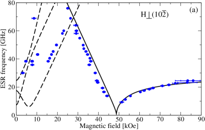
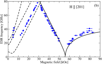
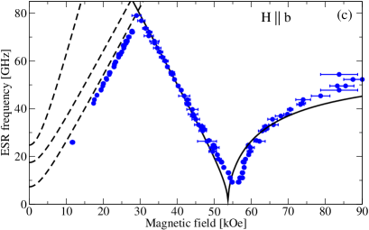
Figure 2: ESR frequency-field dependenciesGlazkov+03 taken at $T=1.5$ K for different field orientations, in comparison with the present theory. Solid and dashed lines correspond to the ground state and thermally activated transitions, respectively.

The best fit to the entire set of the experimental frequency-field dependencies is obtained with

$$\bm{\beta}=\{5.628,5.638,5.635\},\quad\bm{\widetilde{m}}=\{5.725,5.711,5.714\}.$$ (16)

Here all values are given in meV, the absolute error for the anisotropic part of $\bm{\beta}$, $\bm{\widetilde{m}}$ is about $10^{-3}$, but for the isotropic part it is larger, about $0.1$: the results are not very sensitive to a shift of $\beta_{i}$ and $\widetilde{m}_{i}$ by the same value.

We assumed the $g$-factor to be diagonal in the chosen anisotropy axes and took $g_{xx}=2.29$, $g_{yy}=g_{zz}=2.06$. The theoretical curves are shown in Fig. 2 in comparison to the experimental results. All gaps occur at $\bm{q}=0$. Solid lines show the lowest magnon gap, and the dashed ones correspond to the transitions between three branches of the magnon triplet at $q=0$. The theory is in a good agreement with the low-temperature ESR results.

We were not able to estimate $\bm{\alpha}$ from our fit, since the results are insensitive to the exact value of $\alpha_{i}$: indeed, $\bm{\alpha}$ enters only the $\eta^{2}\varphi^{2}$-type part of the interaction (III), and in the ordered phase $\eta\propto(h/J)\varphi$, which suppresses the contribution of such terms in the relevant field range $h/J<0.1$. Available estimatesexcitations of ${J}_{(100)}$, ${J^{\prime}}_{(1{1\over 2}{1\over 2})}$ suggest that $\alpha_{i}-\beta_{i}\approx-0.92$ meV, which has been assumed for the curves presented in Fig. 2.

Above the critical field the lowest gap opens as $E_{g}\simeq C\sqrt{h^{2}-h_{c}^{2}}$, e.g., for $\bm{H}\parallel z$ and weak anisotropy,

$$C^{2}\simeq 2(\widetilde{m}_{y}/m_{y})(\widetilde{m}_{y}m_{x}-\widetilde{m}_{x}m_{y})/(\widetilde{m}_{x}+\widetilde{m}_{y})^{2}\simeq 0.16,$$

where the weak contribution of $\gamma_{ij}$, $\lambda_{ij}$ is neglected.

IV Discussion

Our analysis suggests that the anisotropy in intradimer interactions $\widetilde{m}_{i}$ as well as in inter-dimer couplings $\beta_{i}$ is very small and does not exceed one percent, which is plausible for the exchange anisotropy.note From Eq. (16) one may get the impression that the intradimer exchange has a different sign of anisotropy. However, $\bm{\widetilde{m}}$ given in (16) corresponds to the physical intradimer coupling $\bm{J}=\{5.700,5.728,5.722\}$, so that the anisotropy has the same character for inter- and intradimer exchange: $y$ is the easy axis, and $z=b$ is the intermediate axis.

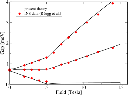
Figure 3: INS results of Rüegg et al.Ruegg+02 ; Ruegg+03 taken at $T=1.5$ K, compared with the present theory. In this geometry ($\bm{H}$ is perpendicular to the plane defined by $(010)$ and $(104)$ vectors) the predicted lowest gap stays below $0.09$ meV at $H>H_{c}$, i.e., beyond the available experimental resolution.

According to our calculations, the staggered order parameter $\bm{\varphi}^{(0)}$ is directed along the $y$ axis for $\bm{H}\parallel\bm{b}$ and $\bm{H}\perp(10\overline{2})$ (with a tiny deviation from the $(yz)$ plane in the latter case); for $\bm{H}\parallel[201]$, we predict that $\bm{\varphi}^{(0)}\parallel\bm{b}$. The magnitude of the order parameter at $H=90$ kOe is about $0.1$ of the saturation value, for all three field geometries. Those predictions agree with the existing results of elastic neutron experiments Tanaka+01 for $H\parallel b$, and can be tested for other orientations. Our results are consistent with the INS dataRuegg+02 ; Ruegg+03 as well, see Fig. 3.

It is worthwhile to note that the same conclusion on the character of the anisotropy ($y$ and $b$ being the easy and the second easy axis) was reached in recent ESR studiesShindo+unpub of the impurity-induced order in $\rm Mg$-doped $\rm TlCuCl_{3}$.

We are grateful to A. Furusaki, H.-J. Mikeska, Ch. Rüegg, A. I. Smirnov, and K. Totsuka for fruitful discussions. This work is supported in part by Grant I/75895 from the Volkswagen-Stiftung, by Grant No. 03-02-16579 from Russian Foundation for Basic Research, by INTAS Grant No. 04-5890, and by Grant-in-Aid for Scientific Research on Priority Areas “Field-Induced New Quantum Phenomena in Magnetic Systems”.

References

- (1) I. Affleck, Phys. Rev. B 41, 6697 (1990); Phys. Rev. B 43, 3215 (1991); S. Sachdev, T. Senthil, and R. Shankar, ibid. 50, 258 (1994); T. Giamarchi and A. M. Tsvelik, ibid. 59, 11398 (1999).
- (2) T. Nikuni, M. Oshikawa, A. Oosawa, and H. Tanaka, Phys. Rev. Lett. 84, 5868 (2000).
- (3) A. Oosawa, M. Ishi, and H. Tanaka, J. Phys.: Condens. Matter, 11, 265 (1999).
- (4) H. Tanaka, A. Oosawa, T. Kato, H. Uekusa, Y. Ohashi, K. Kakurai and A. Hoser, J. Phys. Soc. Jpn., 70, 939 (2001).
- (5) H. Tanaka, T. Takatsu, W. Shiramura et al., Physica B, 246-247, 545 (1998).
- (6) K. Takatsu, W. Shiramura, H. Tanaka et al., J. Magn. & Magn. Mater., 177-181, 697 (1998).
- (7) Ch. Rüegg, N. Cavadini, A. Furrer, H.-U. Güdel, P. Vorderwisch, and H. Mutka, Appl. Phys. A 74, S840 (2002).
- (8) Ch. Rüegg, N. Cavadini, A. Furrer, H.-U. Güdel, K. Krämer, H. Mutka, A. Wildes, K. Habicht, and P. Vorderwisch, Nature 423, 62 (2003).
- (9) M. Matsumoto, B. Normand, T. M. Rice, and M. Sigrist, Phys. Rev. Lett. 89, 077203 (2002).
- (10) V. N. Glazkov, A. I. Smirnov, H. Tanaka, and A. Oosawa, preprint cond-mat/0311243, to appear in Phys. Rev. B.
- (11) A. K. Kolezhuk, Phys. Rev. B 53, 318 (1996).
- (12) A. Zheludev, S. M. Shapiro, Z. Honda, K. Katsumata, B. Grenier, E. Ressouche, L.-P. Regnault, Y. Chen, P. Vorderwisch, H.-J. Mikeska, and A. K. Kolezhuk, Phys. Rev. B 69, 054414 (2003).
- (13) S. Sachdev and R. N. Bhatt, Phys. Rev. B 41, 9323 (1990).
- (14) A. Oosawa, T. Kato, H. Tanaka, K. Kakurai, M. Müller, and H.-J. Mikeska, Phys. Rev. B, 65, 094426 (2002).
- (15) We have checked that introducing anisotropy into only one (intra- or interdimer) set of couplings is not sufficient for the description of the experimental data of Ref. Glazkov+03, .
- (16) There is another solution, and , which yields an even better fit but corresponds to unrealistically large anisotropy (about 10% in the intradimer echange) and was hence discarded.
- (17) Y. Shindo, A. Oosawa, T. Ono, and H. Tanaka (unpublished).