Center of mass rotation and vortices in an attractive Bose gas

Abstract

The rotational properties of an attractively interacting Bose gas are studied using analytical and numerical methods. We study perturbatively the ground state phase space for weak interactions, and find that in an anharmonic trap the rotational ground states are vortex or center of mass rotational states; the crossover line separating these two phases is calculated. We further show that the Gross-Pitaevskii equation is a valid description of such a gas in the rotating frame and calculate numerically the phase space structure using this equation. It is found that the transition between vortex and center of mass rotation is gradual; furthermore the perturbative approach is valid only in an exceedingly small portion of phase space. We also present an intuitive picture of the physics involved in terms of correlated successive measurements for the center of mass state.

I Introduction

The rotational properties of atomic Bose condensed gases have been a matter of intense scientific interest recently. The main role in these studies is played by vortices, which are the manifestations of quantized circulation in the quantum gas in question. However, vortices are by no means the only possible rotational states.

By rotating a condensate in a harmonic trap with a certain frequency $\Omega$ a vortex can be created; when rotating the condensate a bit faster a second vortex appears, and so on Madison2000 . Lattices with a large number of vortices have been experimentally observed in many groups Abo2000 ; Engels2003 . There is an upper limit, however, for the rotation frequency in a harmonic trap. This limit is the trap frequency $\omega$ of the confining trap, above which the center of mass of the condensate is destabilized Rose2002 . Interesting physics has been done by the Boulder group working only slightly below this limit Engels2003 . Having prepared a condensate with a vortex lattice, atoms with low angular momenta are then removed. Reaching the rotation rate $0.95\omega$ a metastable giant vortex with a phase singularity on the order of 50 is observed.

On the other hand, the trap limit can be crossed if the trap is not purely harmonic but the potential has a quartic term also Fetter2001 . The steeper potential makes fast rotation possible and thus gives a tool to test theoretical predictions including multiply quantized vortices Lundh2002 , strongly correlated vortex liquids or Quantum Hall like states Cooper2001 ; Ho2001 . The first experimental studies have already been done at ENS Bretin2003 .

The rotation of a condensate in an anharmonic trap is especially interesting when the effective interactions of the atoms are attractive. It was shown by Wilkin et al. that for weak attractive interactions and a given angular momentum, in the lowest energy state the motion is carried by the center of mass (c. m.) Wilkin1998 . For this state the single-particle reduced density matrix has more than one macroscopic eigenvalue in the laboratory reference of frame. This might indicate that the c.m. rotational state is a fragmented condensate, but actually, the state is Bose condensed if it is viewed in the c. m. frame Pethick2000 . Unfortunately, in a harmonic-oscillator trap this state is never thermodynamically stable because the critical frequency for the excitation is equal to the frequency where the gas is destabilized. An anharmonic term in the trapping potential removes the instability and makes the state of c. m. rotation, as well as vortex states, attainable Us2003 .

In this paper we shall study the rotational states of an attractive zero temperature Bose gas confined in an anharmonic trap. We begin by discussing the nature of the relevant states of motion and perturbation theory in Sec. II. In Sec. III we discuss the validity of different equations of motion. The problem is approached within the ordinary Gross-Pitaevskii (GP) mean field theory in Sec. IV. Section V deals with the correlation properties of the c. m. rotational state at the limit of small anharmonicity. Concluding remarks are made in Sec. VI.

II Hamiltonian and perturbation theory

The Hamiltonian for $N$ atoms with binary s-wave interactions is

$$H=-\frac{\hbar^{2}}{2m}\sum_{i=1}^{N}\frac{d^{2}}{d{\bf r}_{i}^{2}}+\sum_{i=1}^{N}V({\bf r}_{i})+\frac{U_{0}}{2}\sum_{i\neq j}\delta({\bf r}_{i}-{\bf r}_{j})$$ (1)

where the strength of the contact interaction $U_{0}=4\pi\hbar^{2}a/m$ with the scattering length $a$ which is here assumed negative. The external field $V$ consists of a cylindrically symmetric harmonic potential with a small quartic addition in the radial direction:

$$V(r,\theta,z)=\frac{1}{2}m\left[\omega^{2}\left(r^{2}+\lambda\frac{r^{4}}{a_{\mathrm{osc}}^{2}}\right)+\omega_{z}^{2}z^{2}\right].$$ (2)

Here the dimensionless parameter $\lambda$ describes the strength of the anharmonic term and the oscillator length $a_{\mathrm{osc}}$ is defined as $a_{\mathrm{osc}}=(\hbar/m\omega)^{1/2}$.

In Refs. Wilkin1998 ; Mottelson1999 , the harmonically trapped gas ($\lambda=0$) was studied by treating the interaction energy perturbatively, in which case the many-body eigenstates are products of nodeless harmonic-oscillator single-particle eigenstates. Here we shall generalize this approach by including also the anharmonic potential . To this end, we first pass to dimensionless units, where lengths are scaled by $a_{\mathrm{osc}}$ and energies by $\hbar\omega$. We obtain

$$H=-\frac{1}{2}\sum_{i=1}^{N}\frac{d^{2}}{d{\bf r}_{i}^{2}}+\frac{1}{2}\sum_{i=1}^{N}\left(r_{i}^{2}+\lambda r_{i}^{4}\right)+\frac{4\pi g}{2}\sum_{i\neq j}\delta({\bf r}_{i}-{\bf r}_{j}),$$ (3)

where we have defined an effective 2D interaction $g$ by integrating out the $z$-component wave function to obtain $g=\sqrt{\omega_{z}/(2\pi\omega)}a/a_{\mathrm{osc}}$ (this can be done because the radial-axial decoupling is exact in perturbation theory). In the attractive case, $g$ is negative. We shall retain the symbols ${\bf r}$, $H$ etc. for the dimensionless quantities in this section, because no confusion can arise.

A general form for a many-body state in two dimensions is

$$\Psi({\bf r}_{1},\ldots{\bf r}_{N})=\sum_{m_{1},\ldots,m_{N}}c_{m_{1},\ldots,m_{N}}\prod_{j=1}^{N}\phi_{m_{j},0}({\bf r}_{j}),$$ (4)

where $\phi_{mn}({\bf r})$ is the harmonic-oscillator single-particle eigenstate in two dimensions with angular momentum $m$ and radial quantum number $n$; only states with $n=0$ participate in perturbation theory. In the unperturbed case ($\lambda=a=0$), for a given total angular momentum $L$ all states which fulfill $m_{1}+\ldots+m_{N}=L$ with all $m_{j}\geq 0$ (and have no radial nodes, i. e. $n=0$) are degenerate. Thus we have, in principle, to perform degenerate perturbation theory on a vast subspace of Hilbert space (the number of basis states is $(N+L-1)!/[N!(L-1)!]$). However, from physical arguments and known exact results, we obtain guidance to what the relevant candidate states should be.

In the purely harmonic case with finite attractive interactions, the ground-state many-body wave function with angular momentum $L$ and particle number $N$ was found to be Wilkin1998

$$\Psi^{C}_{L}(z_{1},\ldots,z_{N})=\sqrt{\frac{N^{L}}{\pi^{N}L!}}\left(\sum_{j=1}^{N}\frac{z_{j}}{N}\right)^{L}\exp\left({-\sum_{j=1}^{N}|z_{j}|^{2}/2}\right),$$ (5)

where $z_{j}=x_{j}+iy_{j}$ are the particle coordinates. The quantity within parentheses is the c. m. coordinate; therefore, this wave function describes rotation of the c. m.  as already mentioned in the introductory paragraph. We consider this state as the ideal c. m. rotational state.

When instead the anharmonicity $\lambda$ is nonzero and the interactions vanish, it was shown in Ref. Lundh2002 that the ground state is the vortex state

$$\Psi^{v}_{m}(z_{1},\ldots,z_{N})=\prod_{j=1}^{N}\frac{1}{\sqrt{\pi m!}}z_{j}^{m}e^{-|z_{j}|^{2}/2},$$ (6)

which is just a Bose-Einstein condensate containing an $m$-fold quantized vortex, thus having angular momentum $Nm$. Vortex-array states do not come into question because they have a lower density on the average, and are therefore not favored by the attractive interaction.

It should be noted that Eqs. (5) and (6) are the extreme cases where either the interaction or anharmonicity are absent. In a more general context we make the difference between these states in terms of cylindrical symmetry. The vortex state is cylindrically symmetric and the ideal c. m. rotational state corresponds clearly to the nonsymmetric case. Between these two states, however, there is a region of nonsymmetric cases, where the c. m. is in rotation although these states do not correspond to the ideal c. m. rotational case of Eq. (5). The leading instability of the vortex state towards a nonsymmetric state was examined in Ref. Kavo2004 . We include these cylindrically nonsymmetric states into our general definition of c. m. rotational states. Other interpretations are possible, though, see Kavo2004 .

There now remains to compare the energies of the two states (5) and (6) . The interaction energies of the two states were calculated in Ref. Mottelson1999 and amount to

$$\langle\Psi^{C}_{L}|H_{\rm int}|\Psi^{C}_{L}\rangle = gN(N-1),$$

$$\langle\Psi^{v}_{m}|H_{\rm int}|\Psi^{v}_{m}\rangle = gN(N-1)\frac{(2m)!}{(m!)^{2}2^{2m}}$$

$$= gN(N-1)\frac{(2m-1)!!}{(2m)!!}.$$

The absolute magnitude of the interaction energy in the vortex state is smaller than that of the ideal c. m. state, and therefore the latter is favored by the attractive interactions (remember that $g<0$). The quartic energies, on the other hand, are proportional to

$$\langle\Psi^{C}_{L}|\sum r_{j}^{4}|\Psi^{C}_{L}\rangle = N\left(2+4\frac{L}{N}+\frac{L^{2}}{N^{2}}-\frac{1}{N}\frac{L}{N}\right),$$

$$\langle\Psi^{v}_{m}|\sum r_{j}^{4}|\Psi^{v}_{m}\rangle = N(m+1)(m+2),$$ (8)

so that for equal angular momentum, the quartic energy of the vortex state is the lowest.

In the vortex state the angular momentum per particle $m$ can only take on integer values. In contrast, in the ideal c. m. state, $q=L/N$ is only quantized in quanta of $1/N$, so when we pass to the infinite limit $q$ is a continuous variable. At fixed $L$, it is easy to determine the boundary between the rotational phases: the ideal c. m. state is energetically favorable when

$$\frac{\lambda}{2}m<|g|N\left(1-\frac{(2m-1)!!}{(2m)!!}\right).$$ (9)

We have discarded all terms ${\mathcal{O}}(N^{-1})$. For $m=q=1$ the condition for c. m. rotation is $\lambda<|g|N$ and for faster rotation, the regime where the ideal c. m. state is favorable is smaller. Since the right-hand side of Eq. (9) increases slower than the left-hand side as $m$ increases, we conclude that for any given pair of parameters $(\lambda,gN)$, there exists a smallest angular momentum $L$ above which a vortex state is favorable.

We now change variables and work at fixed angular velocity $\Omega$ rather than fixed $L$. In the ideal c. m. state we can simply differentiate the energy:

$$\Omega=\frac{dE}{dL}=1+\lambda(2+q)\Rightarrow q=\frac{\Omega-1}{\lambda}-2.$$ (10)

The critical frequency for the excitation of rotational motion is thus $\Omega_{C}^{cm}=1+2\lambda$, and above this threshold we substitute the above expression for $q$ in order to obtain the energy as a function of $\Omega$:

$$\frac{1}{N}[E_{C}(\Omega,\lambda,g)-\Omega L]=-1+2\Omega-\frac{(\Omega-1)^{2}}{2\lambda}-\lambda-|g|N.$$ (11)

The energy of the vortex state as a function of $m$ is

$$\frac{1}{N}E_{v}(m)=1+m+\frac{1}{2}\lambda(m+1)(m+2)-|g|N\frac{(2m-1)!!}{(2m)!!}.$$ (12)

Comparing Eqs. (11) and (12), the critical angular velocities for the successive vortex states are found to be

$$\Omega^{v}_{C1} = 1+2\lambda+\frac{1}{2}|g|N,$$

$$\Omega^{v}_{C2} = 1+3\lambda+\frac{1}{8}|g|N,$$

$$\Omega^{v}_{C,m} = 1+(m+1)\lambda+|g|N\frac{(2m-3)!!}{(2m)!!}.$$ (13)

For given $gN$, $\lambda$ and $\Omega$ it can now be determined which of the states $\Psi^{C}$ and $\Psi^{v}$ has the lower energy. When $\Omega^{v}_{C1}<\Omega<\Omega^{v}_{C2}$, we find that the ideal c. m. state is favorable if the following equivalent conditions hold:

$$|g|N > 6(\Omega-1)-\frac{(\Omega-1)^{2}}{\lambda}-8\lambda,$$

$$\lambda < \frac{3}{8}(\Omega-1)-\frac{1}{16}|g|N-\sqrt{\frac{1}{64}(\Omega-1)^{2}-\frac{3}{64}|g|N(\Omega-1)+\frac{1}{256}|g|N},$$

$$\Omega < 1+3\lambda-\sqrt{\lambda(\lambda-|g|N)}.$$ (14)

If $\lambda-\sqrt{\lambda(\lambda-|g|N)}<|g|N/2$, then the vortex state is favorable for all $\Omega>\Omega^{v}_{C1}$. If $|g|N>\lambda$, then the ideal c. m. state is the favorable one in the whole interval $\Omega^{v}_{C1}<\Omega<\Omega^{v}_{C2}$ but the vortex state may be favorable for higher frequencies, as discussed above. To summarize the dependencies: (1) a small anharmonic term $\lambda$ favors the ideal c. m.-rotation state; (2) a small interaction term $|g|N$ favors the vortex state; (3) a large angular velocity $\Omega$ favors the vortex state.

III Equations of Motion

The perturbative approach has, naturally, a limited range of validity; as we shall see, it is in fact accurate only for very small values of $gN$ and $\lambda$. There is thus need for a more general scheme and we shall now discuss what kind of approximation can be used to describe the attractive gas.

In a purely harmonic potential the center of mass motion decouples from the internal motion. This is not the case in an anharmonic trap, but there is still an approximate decoupling for weak anharmonicity. By taking advantage of this, and the fact that the internal motion is Bose condensed, coupled equations of motion for the c. m. and internal motion were derived in Ref. Us2003 :

$$\left\{-\frac{\hbar^{2}}{2M}\frac{\partial^{2}}{\partial{\bf R}^{2}}+V_{C}({\bf R})\right\}\psi_{C}({\bf R})=E_{C}\psi_{C}({\bf R}),$$ (15)

$$\left\{-\frac{\hbar^{2}}{2m}\frac{\partial^{2}}{\partial{\bf r}^{2}}+V_{R}({\bf r})+U_{0}|\Phi({\bf r})|^{2}\right\}\Phi({\bf r})=\mu\Phi({\bf r}).$$ (16)

Here, the c. m. is described quantum mechanically by the wave function $\psi_{C}({\bf R})$, and the Bose-Einstein condensed internal motion is governed by the condensate wave function $\Phi({\bf r})$, where ${\bf R}$ is the c. m. coordinate and ${\bf r}$ is the particle coordinate relative to the c. m. The effective potentials for the center-of-mass and relative motion are

$$V_{C}(R)=\frac{1}{2}M\omega^{2}(1+4\lambda\frac{\langle r^{2}\rangle}{a_{\mathrm{osc}}^{2}})R^{2}+\frac{\lambda M\omega^{2}}{2a_{\mathrm{osc}}^{2}}R^{4},$$ (17)

$$V_{R}(r)=\frac{1}{2}m\omega^{2}(1+4\lambda\frac{\langle R^{2}\rangle}{a_{\mathrm{osc}}^{2}})r^{2}+\frac{\lambda m\omega^{2}}{2a_{\mathrm{osc}}^{2}}r^{4},$$ (18)

where $\langle R^{2}\rangle=\int N^{3}d{\bf R}R^{2}|\psi_{C}({\bf R})|^{2}$ and $\langle r^{2}\rangle=N^{-1}\int d{\bf r}r^{2}|\Phi({\bf r})|^{2}$ gives the coupling between the two wave functions. These equations are capable of describing both the (ideal) state of c. m. rotation and vortex states and were used in Ref. Us2003 to find the parameter regimes for those two states of motion. The perturbative results of Sec. II emerge from these equations in the limit $\lambda\to 0,gN\to 0$ if $N$ is assumed large.

Here, we shall take an alternative path to describing the motion of the attractive gases. Namely, we argue that the ordinary Gross-Pitaevskii equation Pethicksmith2001 can be used to describe these rotating systems. The reason is simple: as shown in Ref. Pethick2000 , the state of c. m. rotation is Bose-Einstein condensed according to an observer co-moving with the c. m. Therefore, if we transform to a coordinate system moving with the c. m., we should be able to use the Gross-Pitaevskii equation. But if the cloud is in its ground state, under a rotational force with frequency $\Omega$, the c. m. is also rotating with the frequency $\Omega$ and the coordinate transformation is effected simply by going to a rotating frame as usual Pethicksmith2001 :

$$H\to H^{\prime}=H-\Omega\hat{L},$$ (19)

where $\hat{L}$ is the angular momentum operator. Solving the Gross-Pitaevskii equation in the rotating frame should thus allow us to describe stationary states of the cloud, both in the vortex and the c. m. states. This result comes as a bit of a surprise, considering that in Ref. Wilkin1998 the c. m. state was found not to be Bose-Einstein condensed. We note also that working at fixed $\Omega$ is the correct description of the common experimental approach of letting the cloud equilibrate under the influence of a rotational drive.

Compared with the two coupled wave equations (15-18), the full Gross-Pitaevskii equation is more general: it lifts the restriction of small values of $\lambda$, so that rotational motion in any trap can be described as long as one can move to a reference frame in which the motion is Bose-Einstein condensed. On the other hand, the GPE approach describes the c. m. motion classically instead of quantum mechanically, but this is hardly an issue unless one wishes to specifically study the quantum fluctuations in the c. m. motion. The quantum mechanical c. m. motion will be illustrated in Sec. V.

IV Numerical Simulations

As we argued in the preceeding section, the attractive Bose gas is well described by the single component Gross-Pitaevskii equation in a frame rotating with frequency ${\bf\Omega}$,

$$\left[-\frac{\hbar^{2}}{2m}\nabla^{2}+V\left({\bf r}\right)-{\bf\Omega}\cdot\hat{L}+U_{0}|\Psi\left({\bf r}\right)|^{2}\right]\Psi\left({\bf r}\right)=\mu\Psi\left({\bf r}\right).$$ (20)

To solve this numerically for the anharmonic potential of Eq. (2), we choose $\lambda=0.15$, $N=1000$, $\omega=2\pi\times 30$ Hz, $\omega_{z}=2\pi\times 180$ Hz and the mass of atomic Li⁷. For the harmonic trap frequency much stronger in $z$-direction, we may assume the motion in this direction to be frozen in the ground state of the trap and the problem becomes two-dimensional. The ground state is now found by numerically propagating the time-dependent counterpart of Eq. (20) in imaginary time. The grid size varies from $128\times 128$ points up to $256\times 256$.

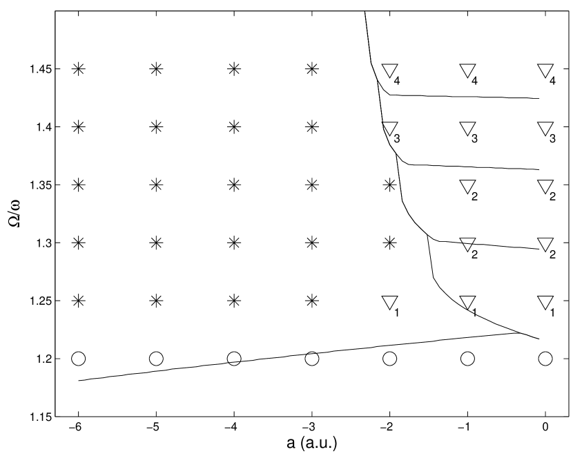
With the fixed parameters mentioned above, we map the ground state phase-space with respect to the rotational frequency and the scattering length. The resulting phase-space diagram is plotted in Fig. 1. The result of the decoupling approximation, Eqs. (15-18), with a Gaussian ansatz for the density Us2003 is also included. We see that the ground state is nonrotating below $\Omega/\omega\approx 1.2$. The cloud just stays at the bottom of the trap with angular momentum $L=0$ (within the numerical uncertainty). As the rotation frequency is increased the ground state depends on the interaction strength. For weak interactions the angular momentum $L/N$ is quantized in integer values that increase with rotation frequency. The ground state is a (multiply) quantized vortex (see Fig. 2). On the contrary, stronger interactions break the rotational symmetry. The circulation is not quantized anymore and the density of the condensate has a shape of a crescent as can be seen from Fig. 2. This configuration corresponds to the c. m. rotational state. For even stronger interactions, the density becomes more concentrated and the cloud attains an approximately ellipsoidal shape residing off center.

Interestingly, the coupled equations of motion (15-18), derived from the factorization of the wave function into c. m. and internal parts, fail to describe the elongated shapes that the cloud attains for moderately strong attraction. The assumptions behind those equations imply, namely, cylindrical symmetry of the condensate wave function. The factorization ansatz thus fails precisely in the situation when the quartic potential has a strong effect on the shape of the cloud, i.e., when we are close to the phase boundary.

Figure 1: The ground state phase-space diagram of a condensate in a rotating trap with $\lambda=0.15$ as a function of the rotating frequency and the scattering length. Different ground states are marked by the following symbols: $\bigcirc$, nonrotating state; $\bigtriangledown$, vortex state (the number is the circulation of a multiply quantized vortex); *, c. m. rotational state. The solid lines give the same phase-space diagram obtained from the equations of motion where the c. m. and internal motion are decoupled, using a Gaussian ansatz for the wave functions.

Figure 2: Density plots for different ground state configurations. Bright shades indicate high density. On the left, we have a doubly quantized vortex for $a=-1.0$ a.u., in the center c. m. rotational state for $a=-4.0$ a.u. and on the right c. m. state for $a=-10.0$ a.u. Anharmonicity is $\lambda=0.15$ and the rotation frequency is fixed to $\Omega/\omega=1.35$. The unit of length for $x$ and $y$ is $\left(\hbar/m\omega\right)^{\frac{1}{2}}$.

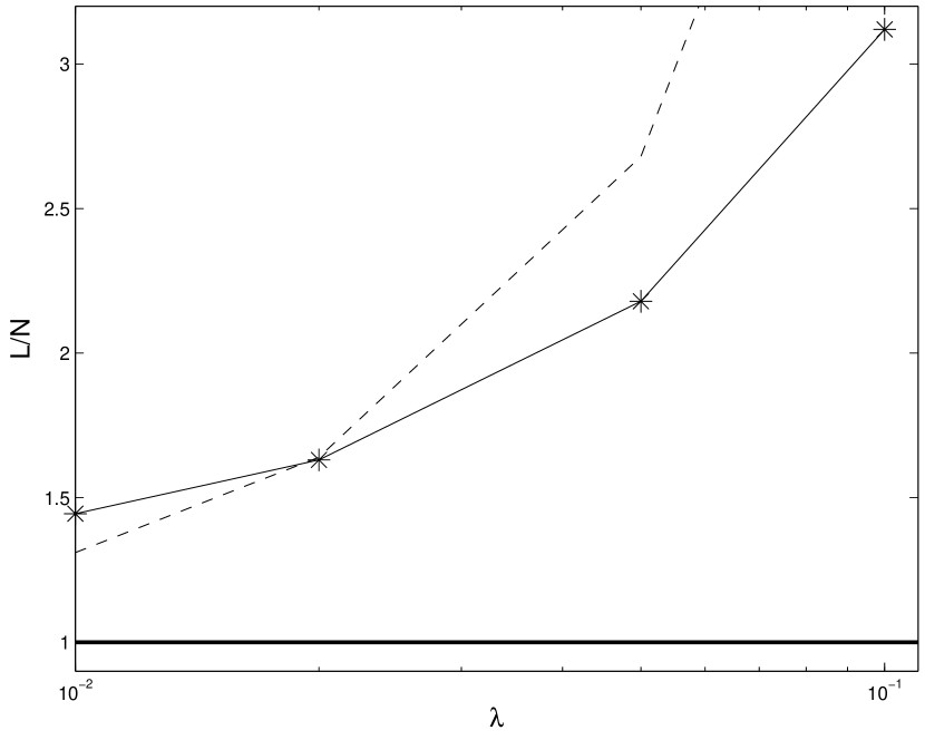
From the perturbative method we have an expression for $q=L/N$ in Eq. (10) as a function of $\Omega$ and $\lambda$. We perform a comparison between this simple perturbative formula for the ideal c. m. state and the GP procedure by choosing the set of these pairs $\left(\Omega,\lambda\right)$ to be such that $q=1$. In Fig. 3 we plot the results from the GP simulations for the angular momentum per atom as a function of $\lambda$. When the anharmonicity gets smaller $q$ seems to approach unity. Still, for the given parameter range the difference between numerical and perturbative results is clear. This is somewhat unexpected, so to verify the numerical results we also plot the corresponding values of $q$ for Gaussian trial wave functions in the coupled Eqs. (15-18). The results are comparable to the ones from GP simulations; this shows that perturbation theory can only be trusted in an extremely small portion of phase space.

Figure 3: The angular momentum (in units of $\hbar$) per atom as a function of the dimensionless anharmonicity parameter $\lambda$ for the c. m. state. The parameter $\Omega/\omega$ is chosen such that in perturbation theory $L/N=1$. Because we compare this to the results from GP simulations (marked by the symbol *) we have to fix the dimensionless interaction parameter $gN$ also. The parameter set for the lowest $\lambda$ is $\left(\lambda=0.01;\Omega=1.03;gN=0.015\right)$ and the others are $\left(0.02;1.06;0.03\right)$, $\left(0.05;1.15;0.075\right)$ and $\left(0.1;1.3;0.15\right)$ respectively. The dashed line is variationally calculated for Gaussian trial wave functions in the decoupling approximation.

That the anharmonic trapping potential is essential for stabilizing these states of motion can be seen from the following argument. The effective potential seen by the rotating atoms is the sum of the actual potential $V(r,\theta,z)$ and the centrifugal term:

$$V_{\rm eff}(r)=\frac{1}{2}m(\omega^{2}-\Omega^{2})r^{2}+\frac{1}{2}m\omega^{2}\lambda\frac{r^{4}}{a_{\mathrm{osc}}^{2}}.$$ (21)

For slow rotation, $\Omega<\omega$, the prefactor of the $r^{2}$ term is positive and the effective potential is just a more shallow anharmonic potential. In that regime there is no rotation for the attractive gas. For rotation faster than the trap frequency, however, the effective potential attains a Mexican-hat shape and the ground-state density distribution lies along the bottom of this toroidal potential. If the trap bottom is deep and the effective trap width is small the condensate is confined in an effectively one-dimensional torus which has been studied analytically in two recent articles Kana2003 ; Kavo2003 . Just as in the present study, two types of state are found in this idealized geometry, termed the uniform-density state and the localized density state (bright soliton). Clearly, the uniform-density state can be identified with our vortex state, and the bright soliton with the c. m. state. The conclusion drawn from the GP analysis is thus that the crossover from vortex to c.m. rotation is gradual, whereas the coupled equations (15-16) predicted a discontinuous crossover Us2003 . In view of the arguments presented in Sec. III to the effect that the GP equation provides a valid description of the gas, the correct conclusion is that the crossover is gradual. This conclusion is supported by the exact findings in the simplified 1D model Kana2003 ; Kavo2003 . The failure of the coupled-equation approach can be ascribed to the fact that it is restricted to cylindrically symmetric density profiles and is thus unable to describe the elongated structures seen in Fig. 2.

To check that the results are not specific to two dimensions, we have solved the GP equation in 3D also. Both ground state configurations are obtained in these simulations. As an example we present a density plot of a c. m. state in Fig. 4. Unfortunately, the computations are too time consuming for a quantitative mapping of the phase-space.

Figure 4: Density plot of a c. m. rotational state obtained by solving 3D GP equation. On the left $z=0$ plane and on the right $y=0$ plane. The relevant parameters are $\Omega/\omega=1.40$, $a=-10.0$ a.u. and $\lambda=0.15$. The unit of length for $x$, $y$ and $z$ is $\left(\hbar/m\omega\right)^{\frac{1}{2}}$.

V Correlation analysis

It is instructive to visualize the dynamics of the many-body wave function Eq. (5) found by Wilkin et al.  Wilkin1998 , to see the connection between the wave function and the result of the numerical Gross-Pitaevskii calculations (Fig. 2). We therefore calculate the outcome of two consecutive measurements, given by the correlation function

$$c\left(z1,z2;t1,t2\right)=\frac{\langle\hat{\psi^{\dagger}}(z_{1},t_{1})\hat{\psi^{\dagger}}(z_{2},t_{2})\hat{\psi}(z_{2},t_{2})\hat{\psi}(z_{1},t_{1})\rangle}{\langle\hat{\psi^{\dagger}}(z_{1},t_{1})\hat{\psi}(z_{1},t_{1})\rangle},$$ (22)

that is, the conditional probability of detecting an atom at $(z_{2},t_{2})$ provided that one was detected at $(z_{1},t_{1})$. Here, we scale the lengths and the energies as we did in Sec. II. The time is scaled by $1/\omega$. By making a multi-nomial expansion, the many-body wave function (5) can be expressed in the terms of single-particle harmonic oscillator eigenstates:

$$\Psi=\sum\sqrt{\frac{N^{L}}{\pi^{N}L!}}\frac{L!}{m_{1}!\cdots m_{N}!}z_{1}^{m_{1}}\cdots z_{N}^{m_{N}}\exp\left(\sum_{i=1}^{N}-|z_{i}|^{2}/2\right)$$ (23)

where the sum is taken over all possible combinations of $\{m_{i}\}$ that fulfill $m_{1}+\cdots m_{N}=L$. This state can now be easily constructed in the second quantized form $|\Psi\rangle=\sum f\left(n_{0},\ldots,n_{L}\right)|n_{0},\ldots,n_{L}\rangle$ where the expansion coefficients are

$$f\left(n_{0},\ldots,n_{L}\right)=\frac{1}{N^{L}}\left(\frac{N!}{n_{0}!\cdots n_{L}!}\right)^{\frac{1}{2}}\left(\frac{L!}{\left(0!\right)^{n_{0}}\cdots\left(L!\right)^{n_{L}}}\right)^{\frac{1}{2}}$$ (24)

and $n_{m}$ denotes the population of atoms in the harmonic oscillator eigenstate of angular momentum $m$.

When the ideal c. m. state is written as a superposition of different distributions of atoms in harmonic oscillator eigenstates, it is natural to determine the correlation (22) by writing the field operators in the harmonic oscillator basis

$$\hat{\psi}(z,t)=\sum_{m=0}^{L}\left(\pi m!\right)^{-\frac{1}{2}}z^{m}\exp\left(-|z|^{2}/2\right)\exp\left(-i(m+1)t\right)\hat{a}_{m}.$$ (25)

Here $\hat{a}_{m}$ is the bosonic particle destruction operator for the state $m$. The form of the time dependent exponential comes from the energy spectrum

$$E=\omega=|m|+2n_{r}+1.$$ (26)

In this case, to minimize the energy, the expansion (23) contains only terms where the radial quantum number $n_{r}$ is zero. We are interested in the dynamics as a function of the polar angle $\theta$ with a fixed distance $R$ from the center of the trap. Hence, we denote $z_{1}=Re^{i\theta_{1}}$ and $z_{2}=Re^{i\theta_{2}}$. In addition we choose $t_{1}=0$, $\theta_{1}=0$, $t_{2}=t$ and $\theta_{2}=\theta$. After doing some algebra, one gets

$$\langle\hat{\psi^{\dagger}}(z_{1},t_{1})\hat{\psi}(z_{1},t_{1})\rangle=\sum_{f}\sum_{m=0}^{L}e^{-R^{2}}f^{2}\left(\pi m!\right)^{-1}R^{2m}n_{m}$$ (27)

for the denominator. The numerator is a bit more tedious but straightforward:

$$\langle\psi^{\dagger}(z_{1},t_{1})\psi^{\dagger}(z_{2},t_{2})\psi(z_{2},t_{2})\psi(z_{1},t_{1})\rangle=$$

$$\sum_{f}\sum_{m=0}^{L}\sum_{m^{\prime}>m}^{L}\sum_{m^{\prime\prime}=0}^{L}\frac{2f^{2}}{\pi^{2}}\frac{n_{m^{\prime}}n_{m}}{m^{\prime\prime}!(m+m^{\prime}-m^{\prime\prime})!}R^{2\left(m+m^{\prime}\right)}e^{-2R^{2}}\cos\left(\left(m-m^{\prime\prime}\right)\left(\theta-t\right)\right)+$$

$$\sum_{f}\sum_{m=0}^{L}\sum_{m^{\prime}=0}^{m-1}\frac{2f^{2}}{\pi^{2}}\left[\frac{n_{m}\left(n_{m}-1\right)}{m^{\prime}!\left(2m-m^{\prime}\right)!}+\frac{n_{m}n_{2m^{\prime}-m}}{\left(m^{\prime}!\right)^{2}}\right]R^{4m}e^{-2R^{2}}\cos\left(\left(m-m^{\prime}\right)\left(\theta-t\right)\right)+$$

$$\sum_{f}\sum_{m=0}^{L}\sum_{m^{\prime}>m}^{L}\frac{2f^{2}n_{m^{\prime}}n_{m}}{\pi^{2}m^{\prime}!m!}R^{2\left(m^{\prime}+m\right)}e^{-2R^{2}}\cos\left(\left(m^{\prime}-m\right)\left(\theta-t\right)\right)+$$ (28)

$$\sum_{f}\sum_{m=0}^{L}\sum_{m^{\prime}>m}^{L}\frac{2f^{2}n_{m^{\prime}}n_{m}}{\pi^{2}m^{\prime}!m!}R^{2\left(m^{\prime}+m\right)}e^{-2R^{2}}+$$

$$\sum_{f}\sum_{m=0}^{L}\frac{f^{2}n_{m}\left(n_{m}-1\right)}{\pi^{2}\left(m!\right)^{2}}R^{4m}e^{-2R^{2}}.$$

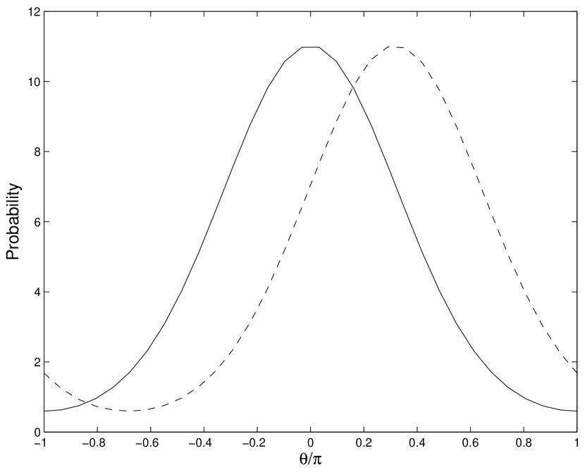
In the first term $m^{\prime\prime}$ must satisfy certain conditions, namely $m^{\prime\prime}\neq m$, $m^{\prime\prime}\neq m^{\prime}$ and $m^{\prime\prime}\neq m+m^{\prime}-m^{\prime\prime}$. By combining (27) and (28), we get a slightly complicated expression for the correlation function (22). To visualize, we plot an example in Fig. 5 for $R=1$. The curves illustrate the conditional probabilities at two different values of $t$ when $N=6$ and $L=6$. As expected it describes a shape retaining a peaked structure moving clockwise at an angular frequency $\Omega=\omega$ (i. e. $\Omega=1$ in dimensionless units).

Figure 5: Probability (unnormalized) of observing an atom at $\theta$ when another atom was detected at $\theta=0$ for $t=0$. The solid line is the time correlation Eq. (22) at $t=0$ and the dashed line represents $t=1.0$. The unit of time is $1/\omega$.

VI Conclusions

In conclusion, we have studied the ground state properties of an attractively interacting zero temperature Bose gas in the presence of an anharmonic trap and a rotational drive. The two different ground state configurations, vortex and center of mass rotation were investigated at the limit when both anharmonicity and interactions are weak. In this limit, analytical conditions for these states to appear were obtained as functions of rotation frequency, anharmonicity and interaction strength. To go beyond the perturbation theory, we have demonstrated that the ground state can be solved by using the ordinary Gross-Pitaevskii equation co-rotating with the external drive. This treatment differs from our previous work Us2003 where the coupled equations of motion were obtained by assuming the many body wave function to be a product of a c.m. wave function and a Bose condensed wave function of the motion relative to the c.m. Here, we treat the motion of the c.m. classically. The Gross-Pitaevskii approach enables us to study any strength of the coupling or anharmonicity. We note that the comparison between different approximative methods shows that the perturbation result is valid for only a very limited parameter range. The extension of the perturbative analysis performed in Ref. Kavo2004 may improve the situation slightly. Finally, we have visualized the c.m. dynamics by studying the correlations of two consecutive measurements.

The rotation of a Bose condensate with repulsive interactions in an anharmonic trap is already experimentally performed Bretin2003 . The condensate was stirred with a laser in a trap which was created by combining a harmonic magnetic potential with an optical potential of Gaussian shape. In principle, by using a similar technique for attractively interacting Bose gas one could be able to observe the rotational ground states we have studied. The possibility to tune scattering lengths with magnetic fields via Feshbach resonances Feshb1992 ; Tiesi1993 offers another tool for probing the parameter space.

VII Acknowledgments

Discussions with C. J. Pethick and G. Kavoulakis are gratefully acknowledged. We also thank J.-P. Martikainen for valuable help in the numerical procedure and M. Mackie for critical reading of the manuscript. The authors acknowledge support from the Academy of Finland (Project 206108), the European Network “Cold Atoms and Ultra-Precise Atomic Clocks” (CAUAC), and the Magnus Ehrnrooth foundation.

References

- (1) K. W. Madison, F. Chevy, W. Wohlleben, and J. Dalibard, Phys. Rev. Lett. 84, 806 (2000).
- (2) J. R. Abo-Shaeer, C. Raman, J. M. Vogels, and W. Ketterle, Science 292, 476 (2001).
- (3) P. Engels, I. Coddington, P. C. Haljan, V. Schweikhard, and E. A. Cornell, Phys. Rev. Lett. 90, 170405 (2003).
- (4) P. Rosenbusch, D. S. Petrov, S. Sinha, F. Chevy, V. Bretin, Y. Castin, G. Shlyapnikov, and J. Dalibard, Phys. Rev. Lett. 88, 250403 (2002).
- (5) A. L. Fetter, Phys. Rev. A 64, 063608 (2001).
- (6) E. Lundh, Phys. Rev. A 65, 043604 (2002).
- (7) N. R. Cooper, N. K. Wilkin, and J. M. F. Gunn, Phys. Rev. Lett. 87, 120405 (2001).
- (8) T.-L. Ho, Phys. Rev. Lett. 87, 060403 (2001).
- (9) V. Bretin, S. Stock, Y. Seurin, and J. Dalibard, Phys. Rev. Lett. 92, 050403 (2004).
- (10) N. K. Wilkin, J. M. F. Gunn, and R. A. Smith, Phys. Rev. Lett. 80, 2265 (1998).
- (11) C. J. Pethick and L. P. Pitaevskii, Phys. Rev. A 62, 33609 (2000).
- (12) E. Lundh, A. Collin, and K.-A. Suominen, Phys. Rev. Lett. 92, 070401 (2004).
- (13) B. Mottelson, Phys. Rev. Lett. 83, 2695 (1999).
- (14) G. M. Kavoulakis, A. D. Jackson, and G. Baym, Phys. Rev. A 70, 043603 (2004).
- (15) C. J. Pethick and H. Smith, Bose-Einstein Condensation in Dilute Gases (Cambridge University Press, Cambridge, 2001).
- (16) R. Kanamoto, H. Saito, and M. Ueda, Phys. Rev. A 68, 043619 (2003).
- (17) G. M. Kavoulakis, Phys. Rev. A 69, 023613 (2004).
- (18) H. Feshbach, Theoretical Nuclear Physics (Wiley, New York, 1992).
- (19) E. Tiesinga, B. J. Verhaar, and H. T. C. Stoof, Phys. Rev. A 47, 4114 (1993).