Electric fields with ultrasoft pseudo-potentials: applications to benzene and anthracene

Abstract

We present density functional perturbation theory for electric field perturbations and ultra-soft pseudopotentials. Applications to benzene and anthracene molecules and surfaces are reported as examples. We point out several issues concerning the evaluation of the polarizability of molecules and slabs with periodic boundary conditions.

I Introduction

Ultrasoft pseudo-potentials (US-PPs) Vanderbilt are employed in large scale electronic structure calculations because they allow precise and efficient simulations of localized $3d$ and $2p$ electrons with plane-waves basis sets. Several ab-initio techniques have been adapted to US-PPs. Important examples comprise the Car-Parrinello molecular dynamics, Laasonen the Berry phase approach to the macroscopic polarization of solids, king-smith the ballistic conductance of open quantum systems, smogunov and also density functional perturbation theory (DFPT). uno ; due ; giapponesi DFPT baroni ; rmp addresses the response of an inhomogeneous electron gas to external perturbations, giving access to the lattice dynamics, to the dielectric, and to the elastic properties of materials. baroni2 DFPT for lattice dynamics with US-PPs has been presented in detail in Refs. uno, ; due, , whereas the treatment of an electric field perturbation and of the dielectric response has been only briefly sketched in the literature. giapponesi The purpose of this paper is to describe our implementation of DFPT for electric field perturbations, to validate it with US-PPs and to apply it to some examples. We calculate the polarizabilities of two molecules, benzene and anthracene, and the dielectric properties of the $(010)$ surface of benzene and of the $(100)$ surface of anthracene. We validate our DFPT implementation with US-PPs in two ways. First we focus on the electronic density induced, at linear order, by an electric field. This density is calculated by DFPT and by a self-consistent finite electric field (FEF) approach. Second, we compare the polarizability inferred from the dipole moment of the induced charge and from the dielectric constant of the periodic solid simulated within the super-cell approach. In both cases we find a very good agreement between DFPT and FEF.

Using plane-waves and pseudo-potentials, as implemented in present codes, it is not possible to study truly isolated molecules or surfaces. A super-cell geometry must be adopted by creating a fictitious lattice made of periodically repeated molecules or slabs (with two surfaces) separated by enough vacuum and the convergence of the calculated properties must be checked against the increase of the size of the vacuum region. In this respect, to converge the dielectric properties is particularly difficult because, due to the long range of electrostatic interactions, periodic boundary conditions may generate a spurious electric field which become negligible only at very large vacuum spacing. In this paper we show that, accounting for this spurious electric field, it is possible to reduce considerably the vacuum needed to converge the polarizability both by DFPT and by FEF.

We note in passing that in solid benzene and anthracene there are two distinct chemical bonds: strong covalent bonds within a single molecule and weak bonds between molecules responsible for the cohesion of the solid. Within density functional theory, in the local density approximation (LDA) or in the generalized gradient approximation (GGA), one cannot account for the van der Waals forces which are important for molecule-molecule interactions and therefore the geometry of the system cannot be determined from energy minimization. Sprik2 ; Hummer However, once the geometry has been adjusted, the other calculated properties often turns out to be reasonably described by LDA or GGA. In this paper, while we allow the geometry of the isolated molecules to be fully relaxed in order to minimize energy, we borrow from experiment wyckoff the orientations of the molecules and the cell sizes for bulk benzene and anthracene. The geometry of the surfaces is assumed to be identical to the truncated bulk.

The outline of the paper is the following: Section II contains an expression for the dielectric constant with US-PPs. Section III describes our implementation of the FEF approach and other technical details. Section IV is devoted to the study of the polarizability of the benzene and anthracene molecules, while in Section V the dielectric properties of slabs of benzene and anthracene are discussed.

II Dielectric constant with ultrasoft pseudo-potentials

The macroscopic dielectric tensor of an insulating solid is defined as: rmp

$$\epsilon_{\alpha\beta}=\delta_{\alpha\beta}+4\pi{dP_{\alpha}\over dE_{\beta}},$$ (1)

$\alpha$ and $\beta$ are Cartesian coordinates and ${dP_{\alpha}\over dE_{\beta}}$ is the derivative of the electronic polarization with respect to the macroscopic screened electric field ${\bf E}$. We neglect atomic relaxations and therefore all our considerations regard the so called “clamped-ions” dielectric constant $\epsilon_{\infty}$ where only the dielectric contribution of electrons is accounted for.

In order to calculate ${dP_{\alpha}\over dE_{\beta}}$, we begin with the derivative of the electronic density with respect to an electric field. With US-PPs, the electronic density is written as:

$$\rho({\bf r})=\sum_{i}\langle\psi_{i}|K({\bf r})|\psi_{i}\rangle$$ (2)

where the sum runs over the occupied states and the kernel $K({\bf r};{\bf r}_{1},{\bf r}_{2})$ is:

$$K({\bf r};{\bf r}_{1},{\bf r}_{2})=\delta({\bf r}-{\bf r}_{1})\delta({\bf r}-{\bf r}_{2})+$$

$$+\sum_{Inm}Q^{\gamma(I)}_{nm}({\bf r}-{\bf R}_{I})\beta^{\gamma(I)}_{n}({\bf r}_{1}-{\bf R}_{I})\beta^{*\gamma(I)}_{m}({\bf r}_{2}-{\bf R}_{I}).$$ (3)

The augmentation functions $Q^{\gamma(I)}_{nm}({\bf r})$ and the projector functions $\beta^{\gamma(I)}_{n}({\bf r})$ are calculated togheter with the PP and are localized about the atoms at position ${\bf R}_{I}$. Vanderbilt

The electronic charge linearly induced by an electric field is therefore:

$${dn({\bf r})\over dE_{\beta}}=2\sum_{i}\langle{d\psi_{i}\over dE_{\beta}}|K({\bf r})|\psi_{i}\rangle+c.c.,$$ (4)

$c.c.$ means complex conjugate.

Using Eq. 4, we get ${dP_{\alpha}\over dE_{\beta}}$ as:

$${dP_{\alpha}\over dE_{\beta}}=-{2e\over N\Omega}\sum_{i}\int d^{3}r\ \langle{d\psi_{i}\over dE_{\beta}}|{r}_{\alpha}K({\bf r})|\psi_{i}\rangle+c.c.,$$ (5)

where the integral is over the volume of the solid, made up of $N$ unit cells of volume $\Omega$. Born-von Kármán boundary conditions are assumed for the wave-functions. The electron charge is $(-e)$.

For convenience, we define the functions $|\phi_{i}^{\alpha}\rangle=\int d^{3}r\ e{r}_{\alpha}K({\bf r})|\psi_{i}\rangle$, and introduce the projector into the empty states manifold $P_{c}=\sum_{c}|\psi_{c}\rangle\langle\psi_{c}|S$, where $S$ is the overlap matrix (see below). With these definitions, Eq. 5 becomes:

$${dP_{\alpha}\over dE_{\beta}}=-{2\over N\Omega}\sum_{i}\langle{d\psi_{i}\over dE_{\beta}}|P_{c}^{\dagger}|\phi_{i}^{\alpha}\rangle+c.c..$$ (6)

The functions $|\phi_{i}^{\alpha}\rangle$ and hence ${dP_{\alpha}\over dE_{\beta}}$ are well defined in a finite system. In a periodic solid $P_{c}^{\dagger}|\phi_{i}^{\alpha}\rangle$ can be defined as done with norm conserving pseudo-potentials. We exploit the relation between the off-diagonal matrix elements of the ${\bf r}$ operator between non-degenerate Bloch states, and the matrix elements of the velocity operator. With US-PPs, we have:

$$\langle\psi_{j}|S{r}_{\alpha}|\psi_{i}\rangle={\langle\psi_{j}|\left[H-\varepsilon_{i}S,{r}_{\alpha}\right]|\psi_{i}\rangle\over\varepsilon_{j}-\varepsilon_{i}},$$ (7)

where $H$ is the unperturbed Hamiltonian and $\varepsilon_{i}$ are the unperturbed eigenvalues. The overlap matrix $S$ is Vanderbilt

$$S({\bf r}_{1},{\bf r}_{2})=\delta({\bf r}_{1}-{\bf r}_{2})+\sum_{Inm}q^{\gamma(I)}_{nm}\beta^{\gamma(I)}_{n}({\bf r}_{1}-{\bf R}_{I})\beta^{*\gamma(I)}_{m}({\bf r}_{2}-{\bf R}_{I}),$$ (8)

where the coefficients $q^{\gamma(I)}_{nm}=\int{\it d^{3}r}\ Q^{\gamma(I)}_{nm}({\bf r})$ are the integrals of the augmentation functions.

Using Eq. 7, we see that $P_{c}{r}_{\alpha}|\psi_{i}\rangle$ are the solutions of the linear system:

$$\left[H+Q-\varepsilon_{i}S\right]P_{c}{r}_{\alpha}|\psi_{i}\rangle=P_{c}^{\dagger}\left[H-\varepsilon_{i}S,{r}_{\alpha}\right]|\psi_{i}\rangle,$$ (9)

where both the left and the right hand sides are lattice periodic. $Q$ is added to the linear system in order to make it non singular as explained in detail in Ref. rmp, (See Eq. 30 and Eq. 72). With norm conserving pseudopotentials, in insulators, $Q$ is proportional to the valence band projector. Its generalization to US-PPs is given in Ref. due, (see discussion after Eq. 29). By solving this linear system, we obtain $P_{c}{r}_{\alpha}|\psi_{i}\rangle$, while we need $P_{c}^{\dagger}{r}_{\alpha}|\psi_{i}\rangle$ to compute $P_{c}^{\dagger}|\phi_{i}^{\alpha}\rangle$. Since $SP_{c}=P_{c}^{\dagger}S$, we have $SP_{c}{r}_{\alpha}|\psi_{i}\rangle=P_{c}^{\dagger}S{r}_{\alpha}|\psi_{i}\rangle$, hence the functions $P_{c}^{\dagger}|\phi^{\alpha}_{i}\rangle$ are:

$$P_{c}^{\dagger}|\phi_{i}^{\alpha}\rangle=SP_{c}e{r}_{\alpha}|\psi_{i}\rangle-P_{c}^{\dagger}\sum_{Inm}q^{\gamma(I)}_{nm}|\beta_{n}^{I}\rangle\langle\beta_{m}^{I}|e{r}_{\alpha}|\psi_{i}\rangle+P_{c}^{\dagger}\sum_{Inm}{I^{\alpha}_{Inm}}|\beta_{n}^{I}\rangle\langle\beta_{m}^{I}|\psi_{i}\rangle,$$ (10)

where we defined the integral $I^{\alpha}_{Inm}=\int d^{3}r\ e{r}_{\alpha}Q^{\gamma(I)}_{nm}({\bf r}-{\bf R}_{I})$.

To proceed further, we need the first order derivative of the electronic wave-functions $|\psi_{i}\rangle$ with respect to an electric field. We can calculate these quantities to linear order in perturbation theory. The overlap matrix $S$ does not depend on the electric field while the differentiation of the Kohn and Sham potential yields:

$${dV_{KS}\over dE_{\beta}}=\int d^{3}r\left[e{r}_{\beta}+{dV_{Hxc}({\bf r})\over dE_{\beta}}\right]K({\bf r}),$$ (11)

where $V_{Hxc}$ is the Hartree and exchange and correlation potential. Applying $P_{c}^{\dagger}$ to Eq. (19) of Ref. due, , we obtain:

$$\left[H+Q-\varepsilon_{i}S\right]P_{c}|{d\psi_{i}\over dE_{\beta}}\rangle=-P_{c}^{\dagger}\int d^{3}r\left[e{r}_{\beta}+{dV_{Hxc}({\bf r})\over dE_{\beta}}\right]K({\bf r})|\psi_{i}\rangle.$$ (12)

The self-consistent solutions of this linear system, together with Eq. 10, are substituted into Eq. 6 to calculate ${dP_{\alpha}\over dE_{\beta}}$. Finally, the dielectric tensor is calculated via Eq. 1.

III Technical details

We validate the theory by comparison with a self-consistent FEF method. A FEF is simulated as suggested by Kunc and Resta: KR1 ; KR2 a sawtooth-like potential is added to the bare ionic potential. This method, when applied to periodic systems, is not as efficient as other recent approaches Nunes ; Fernandez ; Vanderbiltef ; Pasquarello ; Umari because it requires the simulation of a super-cell, but its implementation is simple. Our systems, molecules and slabs, require already a super-cell and the method of Kunc and Resta suits adequately our goals. The molecules and the slabs are inserted in the region where the sawtooth-like potential is linear like the potential of an electric field (${\bf E}_{sl}$): $\Phi({\bf r})=-{\bf E}_{sl}\cdot{\bf r}$. To ensure periodicity, the slope of the potential is reversed in a small region in the middle of the vacuum. For finite super-cells and small enough fields, the electrons are only slightly polarized by the field, the systems maintain a well defined energy gap between occupied and empty electronic states and electrons do not escape into the vacuum. In these simulations, the macroscopic electric field ${\bf E}$ is zero because, solving the Poisson equation we assume, as a boundary condition, the periodicity of the Hartree potential. The sawtooth-like potential describes a microscopic electric field ${\bf E}_{sl}$ which vanishes averaging over macroscopic distances. On our finite systems, this microscopic field has the same effect of a macroscopic electric field. Indeed, in DFPT, as derived in previous Section, the perturbation is a genuine macroscopic electric field ${\bf E}$ and, as shown in the following, the electronic density induced, at linear order, by the field ${\bf E}_{sl}$ and the electronic density induced by the macroscopic electric field ${\bf E}$ are equal to each other when ${\bf E}_{sl}={\bf E}$.

Both the FEF approach and DFPT for US-PPs have been implemented in the PWscf PWSCF package. All calculations are carried out within the GGA approximation. The expression of the exchange and correlation energy introduced by Perdew, Burke and Ernzerhof (PBE) PBE is used in the GGA functional. The US-PPs of hydrogen and carbon have the parameters described in Ref. due, . Plane waves up to an energy cutoff of 30 Ry for the wave-functions and 180 Ry for the electron density, are used. Only the $\Gamma$ point is used for the Brillouin zone (BZ) sampling in the molecular calculation while a $3\times 3$ Monkhorst and Pack mesh MP of ${\bf k}$-points is used for sampling the two-dimensional BZ of the slabs.

IV Molecules

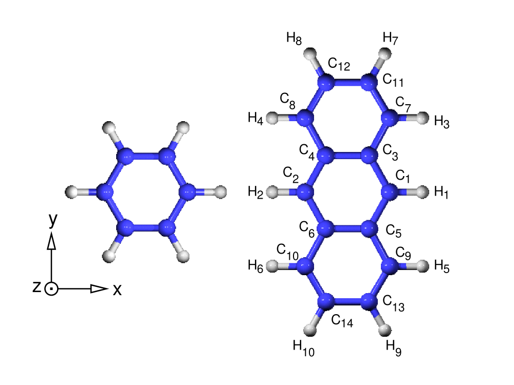
Figure 1: Benzene and anthracene molecules. Distances and angles are reported in Tables 1 and 2 for benzene and anthracene respectively. The polarizability tensors are given with respect to the axes shown in the figure.

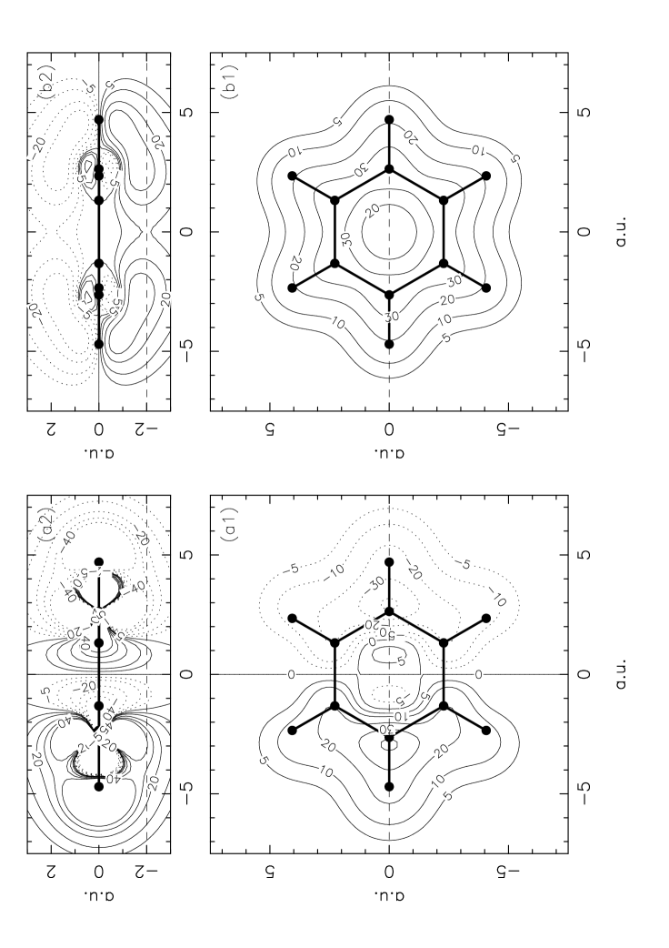
Figure 2: Electronic density induced by an electric field either parallel (a) or perpendicular (b) to the plane of benzene calculated by DFPT. (1) Plane perpendicular to the $z$ axis passing through $(0.0,0.0,-2.0)$ a.u.; (2) plane $xz$. Contours are in units of $10^{-3}$ elec./(a.u.)³. The contours correspond to a field $0.5$ a.u. ($2.57\times 10^{9}$ V/cm).

	this work (PBE)	Ref. JCP-Dele, (B3LYP)	Ref. wyckoff, (expt.)
$C-C$	1.396	1.399	1.398 (n), 1.392 (x)
$C-H$	1.091	1.092	1.090 (n)

Table 1: Theoretical GGA optimized geometry of the benzene molecule compared with previous theoretical work JCP-Dele (B3LYP with localized basis set) and experiment. wyckoff Bond lengths are in Å. The symbols are defined in Fig. 1. Abbreviations: (n) neutron, (x) x-ray diffraction.

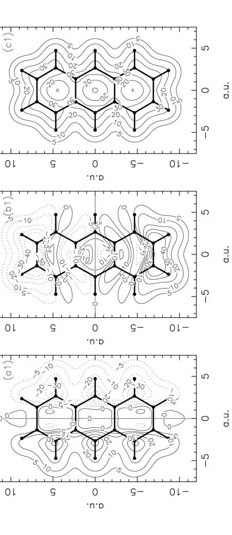
Figure 3: Electronic density induced by an electric field either parallel (a,b) or perpendicular (c) to the plane of anthracene calculated by DFPT. In (a) the field is parallel to the short axis, in (b) it is parallel to the long axis of the molecule. The plane is perpendicular to the $z$ axis passing through the point $(0.0,0.0,-2.0)$ a.u.. Contours are in units of $10^{-3}$ elec./(a.u.)³. The contours correspond to a field $0.5$ a.u..

bond	this work (PBE)	Ref. JCP-Dele, (B3LYP)	Ref. Ketkar, (expt.)	Ref. wyckoff, (expt. solid)
$C_{1}-C_{3}$	1.398	1.403	1.392	1.403
$C_{3}-C_{7}$	1.425	1.432	1.437	1.445
$C_{7}-C_{11}$	1.370	1.372	1.397	1.374
$C_{3}-C_{4}$	1.446	1.447	1.437	1.425
$C_{11}-C_{12}$	1.421	1.428	1.422	1.412
$C_{1}-H_{1}$	1.092	1.094	-	1.121
$C_{11}-H_{7}$	1.090	1.092	-	1.139
$C_{7}-H_{3}$	1.091	1.093	-	1.153
angle
$C_{3}C_{1}C_{5}$	121.74	121.80	-	120.37
$C_{3}C_{7}C_{11}$	120.89	120.97	-	120.31
$H_{3}C_{7}C_{11}$	120.55	120.53	-	123.48
$H_{7}C_{11}C_{12}$	119.34	119.43	-	124.93

Table 2: Theoretical GGA optimized geometry of the anthracene molecule compared with previous theoretical work JCP-Dele (B3LYP with localized basis set) and experiment. Ketkar The experimental geometry of solid anthracene is also reported for comparison. wyckoff Bond lengths are in Å, angles in degrees. The symbols are defined in Fig. 1.

Figure 4: Density profiles along the line ($\lambda$,0.0,$-$2.0) a.u., $-$12 a.u.$<\lambda<$12 a.u., (dashed line) and the difference between DFPT and FEF (continuous line). Upper panel for benzene in a cubic super-cell with size 24 a.u. The lower panel for anthracene in an orthorhombic super-cell with sizes 24 a.u. $\times$ 36 a.u. $\times$ 15 a.u..

	Benzene			Anthracene
$L$ (a.u.)	$\alpha_{xx}$	$\alpha_{zz}$	$\alpha_{xx}$	$\alpha_{yy}$	$\alpha_{zz}$
20	83.6 (87.4)	44.7 (45.7)	—	—	—
24	83.5 (85.7)	44.9 (45.5)	170 (179)	317 (351)	85.5 (87.8)
28	83.5 (84.8)	44.9 (45.3)	171 (177)	313 (333)	86.3 (87.8)
30	83.5 (84.6)	45.0 (45.3)	172 (176)	310 (327)	86.6 (87.9)
32	83.4 (84.3)	45.0 (45.2)	172 (176)	309 (322)	86.8 (87.8)
50	—	—	172 (173)	306 (309)	86.5 (86.8)

Table 3: Independent components of the molecular polarizability tensor of benzene and anthracene (in a.u.) calculated from the dipole moment of $-e\Delta n$ including Lorentz field corrections. Values in parenthesis are calculated neglecting Lorentz field corrections.

	Benzene			Anthracene
$L$ (a.u.)	$\epsilon_{xx}\ (\alpha_{xx})$	$\epsilon_{zz}\ (\alpha_{zz})$	$\epsilon_{xx}\ (\alpha_{xx})$	$\epsilon_{yy}\ (\alpha_{yy})$	$\epsilon_{zz}\ (\alpha_{zz})$
20	1.1372 (83.5)	1.0716 (44.5)	—	—	—
24	1.0778 (83.4)	1.0412 (44.7)	1.1625 (170)	1.3329 (330)	1.0793 (85.0)
28	1.0485 (83.3)	1.0259 (44.8)	1.1013 (171)	1.1908 (313)	1.0501 (86.1)
30	1.0393 (83.3)	1.0210 (44.8)	1.0819 (171)	1.1519 (311)	1.0407 (86.3)
32	1.0323 (83.3)	1.0173 (44.9)	1.0673 (171)	1.1233 (309)	1.0335 (86.5)

Table 4: Dielectric constant of benzene and anthracene molecules in a cubic super-cell as a function of the box size. In parenthesis we report the polarizability (in a.u.) obtained from Eq. 13.

$\alpha_{xx}$	$\alpha_{yy}$	$\alpha_{zz}$	$\bar{\alpha}$	Method/reference
Anthracene
164	287	81.2	177	APSC + B3LYP/6-311G(d,p) Soos
158	266	81.8	167	APSC + MP2 corrections Soos
172	303	86.5	187	APSC + TZVP-FIP Soos
171	306	86.8	188	this work (GGA-PBE)
191	337	96.2	208	DFT with TZVP-FIP basis Reis
169	240	105	171	EFNMR - BS (static)pol-nmr
173	238	103	171	KE, EP, CME - BS (dynamic)Cheng-AJC
165	242	107	171	KE, EP, EST - BS (dynamic)LeFevre
174	272	80.3	175	CR (dynamic) Vuks
139	292	115	182	CR (dynamic) Bounds-ChP
Benzene
74.2		39.5	62.6	HF pol-mp2
76.0		41.3	64.4	HF + MP2 pol-mp2
76.8		37.2	63.6	HF with DZP’ basis Perez-JMS
78.2		37.2	64.5	as above + MP2 Perez-JMS
79.5		45.2	68.1	HF with POL basis Perez-JMS
81.6		45.2	69.5	as above + MP2 Perez-JMS
83.4		45.0	70.6	this work (GGA-PBE)
83.7		44.9	70.9	LDA, Gaussian basis pol-dft
85.0		45.6	72.2	as above - different basis pol-dft
74.9		49.9	66.6	Ref. LeFevre,
74.9		50.6	66.8	KE, EP, CME (dynamic) Cheng-AJC,

Table 5: Theoretical and experimental values of benzene and anthracene polarizabilities. All values are in atomic units. Abbreviations: Atomic polarizability in a self-consistent local field (APSC), benzene solution (BS), Kerr effect (KE), Cotton-Mouton effect (CME), electron polarization (EP), crystal refraction (CR), empirical estimate (EST), Hartree-Fock (HF), Møller-Plesset correction of 2nd order (MP2).

Benzene (C₆H₆) and anthracene (C₁₄H₁₀) are planar molecules, their geometries are shown in Fig. 1. We optimize the geometries and our theoretical bond lengths and angles are reported in the Tabs. 1 and  2 and compared with previous calculations JCP-Dele and with experiment. Ketkar Overall, the agreement between theory and experiment is good and our values compare well also with the more precise B3LYP results. JCP-Dele

As a first test of DFPT, we calculate the electronic density $\Delta n={dn\over dE}E$ induced at linear order by an electric field. Fig. 2 (Fig. 3) shows the density induced in benzene (anthracene) by an electric field either parallel or perpendicular to the molecular plane. The same $\Delta n$ has been calculated by FEF via a numerical differentiation of the self-consistent density with $|{\bf E}_{sl}|=10^{-3}$ a.u. and $|{\bf E}_{sl}|=0$ a.u.. In all cases, to the scale of the figures, the $\Delta n$ calculated by DFPT and the $\Delta n$ calculated by FEF coincide. In Fig. 4 we report, as an example, the difference between two $\Delta n$ to an enlarged scale. This error is due to nonlinear effects (present in the FEF results but not in DFPT) as well as to numerical noise. Its magnitude, lower than 1% of $\Delta n$, is similar with norm-conserving PPs.

Now we can address the molecular polarizabilities. The polarizability of a molecule is a tensor which measures, at linear order, the tendency of the molecule to change its dipole moment when inserted into an electric field. It is defined by the relationship ${\bf p}_{\alpha}=\sum_{\beta}\alpha_{\alpha\beta}{\bf E}_{loc,\beta}$, between the dipole moment ${\bf p}$ of the induced charge density, and ${\bf E}_{loc}$ the electric field acting on the molecule. In general, the polarizability tensor $\alpha$ can be made diagonal in the principal axes. The point group of benzene, $D_{6h}$, and of anthracene, $D_{2h}$, are centrosymmetric, hence these two molecules have no permanent dipole moment. Their principal axes are shown in Fig. 1. In these axes, $\alpha$ has two independent components in benzene ($\alpha_{xx}=\alpha_{yy}$ parallel and $\alpha_{zz}$ perpendicular to the molecular plane), and three independent components in anthracene ($\alpha_{xx}$, $\alpha_{yy}$, $\alpha_{zz}$, parallel to the short molecular axis, parallel to the long molecular axis and perpendicular to the molecular plane, respectively). We first extract the polarizabilities from the dipole moment of the induced charge density $-e\Delta n$. As shown in Figs. 2 and 3, the $\Delta n$ induced in our molecules are localized and well separated by their periodic images, so that ${\bf p}$ can be calculated by a numerical integration (${\bf p}=-e\int\Delta n({\bf r}){\bf r}\ d^{3}r$) over the super-cell volume. The small differences between induced charges calculated by DFPT and by FEF lead to differences smaller than $1\%$ in the dipole moments (for instance, in benzene, for $L=24$ a.u. and $E=0.5$ a.u., $p_{x}=42.79$ a.u. with DFPT and $p_{x}=42.85$ a.u. with FEF). The polarizabilities differ also by less than $1\%$ because, at linear order, ${\bf E}_{loc}$ acting on the molecules is the same. Indeed, the local field can be estimated recognizing that the periodic solid simulated in the super-cell approach, has a macroscopic polarization ${\bf P}={\bf p}/\Omega$. Hence, the local field which acts on the molecules is given by the Lorentz formula ${\bf E}_{loc}={\bf E}_{sl}+{4\pi\over 3}{\bf P}$ (FEF) or ${\bf E}_{loc}={\bf E}+{4\pi\over 3}{\bf P}$ (DFPT). Of course, these formulas are valid for isotropic solids and cubic super-cells, however the isotropic formula is sufficient to correct the main effects of the periodic boundary conditions when the electric field is parallel to one principal axis and the super-cell is cubic. We evaluate the dipole moment of benzene and anthracene for several sizes of the box. In Tab. 3, we report the polarizabilities calculated with or without the Lorentz corrections. In benzene, with a super-cell of $20$ a.u. and a polarizability $\alpha_{xx}=83.6$ a.u., the local field is $4.4\%$ larger than $E_{sl}$ or $E$. In our largest super-cell ($L=32$ a.u.) the local field is still $1\%$ larger than $E_{sl}$ or $E$. From Tab. 3 we can see that the inclusion of the Lorentz correction increases the convergence rate of $\alpha_{xx}$ and $\alpha_{zz}$. A box of $20$ a.u. is sufficient to give values converged within $1\%$. The anthracene molecule is about $18$ a.u. long in the $y$ direction and therefore the molecules can be considered as truly isolated only for super-cell sizes larger than $28$ a.u.. At smaller box sizes, not only electrostatic, but also direct molecule-molecule interactions are important. At $L=28$ a.u., including the Lorentz correction, $\alpha_{xx}$ and $\alpha_{zz}$ are already converged within $1\%$. $\alpha_{yy}$ is instead more difficult to converge. A super-cell of about $50$ a.u. is needed to reduce the local field effects below $1\%$. Instead, including Lorentz corrections, a box size of $32$ a.u. is sufficient to converge $\alpha_{yy}$ within $1\%$.

Besides the direct approach, molecular polarizabilities can be evaluated also starting from the dielectric constant (Eq. 1) of the periodic solid simulated in the super-cell approach. The anisotropic Clausius-Mossotti formula which derives from the approximate Lorentz field given above is: an-cm

$$\alpha_{\alpha\alpha}={3\Omega\over 4\pi}{\epsilon_{\alpha\alpha}-1\over\epsilon_{\alpha\alpha}+2}.$$ (13)

In Tab. 4, we report the dielectric constant as a function of the super-cell size and the polarizabilities calculated via Eq. 13, for both molecules. The convergence rate of the polarizabilities is similar to the convergence rate found in Tab. 3 including the Lorentz field. In all cases the difference of the final polarizabilities in Tab. 3 and in Tab. 4 is below $1\%$.

The final calculated components of the benzene polarizabilities are $\alpha_{xx}=83.4$ a.u. and $\alpha_{zz}=45.0$ a.u.. These values give a mean polarizability $\bar{\alpha}=\frac{1}{3}(2\alpha_{xx}+\alpha_{zz})=70.6$ a.u. and are in good agreement with the results of previous theoretical works and with experiment. We report in Tab. 5 previous theoretical data and experimental values. For anthracene we get $\alpha_{xx}=171$ a.u., $\alpha_{yy}=306$ a.u., $\alpha_{zz}=86.8$ a.u.. These values give a mean polarizability $\bar{\alpha}=188$ a.u.. Experimental values of the anisotropic components of the polarizability of anthracene exist for both diluted benzene solutions and for solid anthracene. The values of $\alpha_{xx}$ ranges from $139$ a.u. to $174$ a.u., $\alpha_{yy}$ between $238$ a.u. and $292$ a.u. and $\alpha_{zz}$ between $80$ a.u. and $115$ a.u. (see Tab. 5). Note that the ionic contribution to the polarizability, which is not accounted for in our calculation, is present in the experiment of Ref. pol-nmr, but not in those of Refs. Cheng-AJC, ; LeFevre, . However it has been estimated that the ionic contribution is only of the order of $5\%$. pol-nmr

V Surfaces

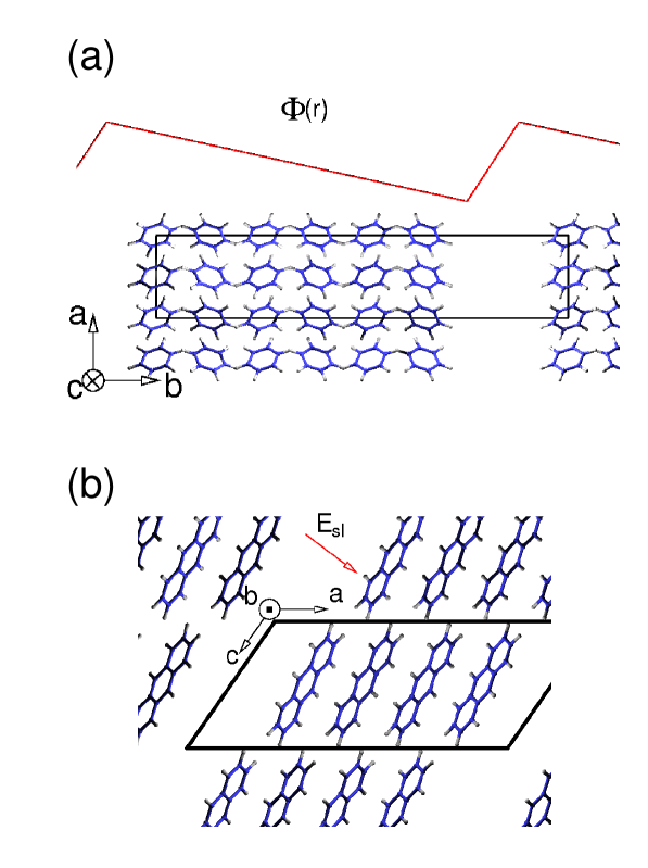
Figure 5: Geometry of the benzene (a) and anthracene (b) slabs. The unit cell is shown by a black frame. In (a) the applied sawtooth–like potential is also indicated.

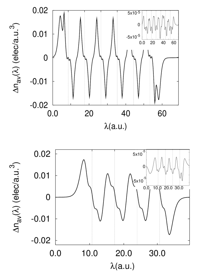
Figure 6: Planar average $\Delta n_{av}$ of the electron density induced by an electric field on the benzene slab (upper panel) and anthracene slab (lower panel). The difference between DFPT and FEF is shown in the insets. $\Delta n$ corresponds to an electric field of $0.5$ a.u.. Vertical lines indicate the position of the centers of the molecules in each layer.

Figure 7: Benzene slab polarizability as a function of the number of layers. The data are interpolated with a linear fit (see Eq. 20).

	Benzene			Anthracene
$L$ (a.u.)	$\alpha$ (Eq. 16)	$\alpha$	$L$ (a.u.)	$\alpha$ (Eq. 16)	$\alpha$
65.0	500.7	1116	36.17	298.6	523.9
68.9	500.9	1044	39.46	298.0	491.3
75.0	500.9	959.8	42.75	298.1	468.2
80.0	500.9	907.9	46.03	298.1	449.9
85.0	500.9	866.5	49.32	298.1	435.1

Table 6: Polarizability of the benzene and anthracene slabs (in a.u.) as a function of the size of the super-cell. Values corrected for the electric field due to the periodic boundary conditions and uncorrected values are both reported.

Some surfaces of molecular crystals can be cleaved by cutting only weak molecule-molecule bonds. Such surfaces are expected to remain insulating and to have dielectric properties similar to the bulk. In this section, we present the dielectric properties of two of these surfaces: the $(010)$ surface of benzene and the $(100)$ surface of anthracene. Moreover, we show how to calculate the dielectric properties of a single slab from the dielectric constant of the solid simulated in the super-cell approach.

The $(010)$ benzene surface is simulated by a six-layers slab and two molecules per layer (see Fig. 5a). The super-cell is orthorhombic with sizes $13.78$ a.u. $\times L$ a.u. $\times 12.74$ a.u., where $L$ depends on the vacuum between slabs. The $(100)$ surface of anthracene is described by a four-layers slab and one molecule per layer (see Fig. 5b). The super-cell is monoclinic with sizes $|{\bf a}|=L/sin\gamma$, $|{\bf b}|=11.41$ a.u. and $|{\bf c}|=21.14$ a.u., where the angle between ${\bf a}$ and ${\bf c}$ is $\gamma=124.7^{\circ}$. The long axis of the molecules is approximately parallel to the ${\bf c}$ vector. Fig. 5a shows the shape of the sawtooth-like potential used in the FEF simulations. The applied field is normal to the surface, in the direction $(010)$ in benzene and in the direction of ${\bf b}\times{\bf c}$ in anthracene. The band structures of these slabs have been reported in Ref. noi, .

We begin by a comparison of the induced electronic density calculated by DFPT and by FEF. In order to visualize the induced density, we introduce the planar average of $\Delta n$, defined as $\Delta n_{av}(\lambda)={1/S}\int_{S}\Delta n({\bf r})\ dS$. Here $\lambda$ is a coordinate along the surface normal and $S$ is the area of one surface unit cell. The integration is on cross sections parallel to the surface. In Fig. 6, we report $\Delta n_{av}$ calculated by DFPT and by FEF. In the latter case the numerical differentiation is done taking the field $E_{sl}=10^{-3}$ a.u. and $E_{sl}=0$ a.u. in benzene and $E_{sl}=2\times 10^{-3}$ a.u. and $E_{sl}=0$ a.u. in anthracene. To the scale of the figure the planar averages calculated by FEF or by DFPT coincide. The error, reported to an enlarged scale in the insets, is always lower than $1\%$ of the value of $\Delta n_{av}$.

Now we move on to the dielectric properties of the slabs. We begin by extracting the polarizability of the slab from the induced dipole moment per unit surface. We define the polarizability of a slab $\alpha$, starting from the relationship:

$$m={\alpha\over S}E_{loc},$$ (14)

where $m=-e\int_{-\infty}^{\infty}\Delta n_{av}(\lambda)\lambda\ d\lambda$ is the induced dipole moment per unit surface area and $E_{loc}$ is the electric field, perpendicular to the surface, which induces the dipole moment on the slab ($E_{loc}$ is the uniform electric field that remains in the vacuum between two slabs after subtraction of all short range inhomogeneous fields). In a periodic slab geometry, the dipole moment of the slab is the origin of a sizable electric field. Actually, as described in Refs. Bengtsson, ; Vanderbilt2, , in an isolated slab a dipole moment per unit surface area produces an the electrostatic potential which has different constant values in the vacuum on the left and on the right part of the slab. In a repeated slab geometry, this jump cannot be accomodated with periodic boundary conditions. Therefore, an artificial uniform electric field appears in the super-cell in order to restore the periodicity of the electrostatic potential. Before applying Eq. 14, this field has to be added to $E_{sl}$ or to $E$ in order to calculate $E_{loc}$ which actually induces the dipole moment on the slab. As in Refs. Bengtsson, ; Vanderbilt2, we evaluate $E_{loc}$ as:

$$E_{loc}=E_{0}+{4\pi m\over L},$$ (15)

where $L$ is the length of the super-cell in the direction perpendicular to the surface and either $E_{0}=E_{sl}$ (FEF) or $E_{0}=E$ (DFPT). Using Eqs. 14 and 15, we calculate the polarizability of a slab from the dipole moment per unit surface area as:

$$\alpha={\Omega\over 4\pi}{x\over 1+x},$$ (16)

where $x=4\pi m/(LE_{0})$. In Tab. 6, we report $\alpha$ calculated by Eq. 16 and compare with $\alpha$ obtained without including the field due to the periodic boundary conditions ($\alpha=Sm/E_{0}$). It is found that the polarizability calculated by Eq. 16 is already converged at the smallest vacuum space for both benzene and anthracene. Tab. 6 shows that the field due to the periodic boundary conditions has the same magnitude of the applied electric field. For instance, in benzene (anthracene), at the minimum slab-slab distance, for $L=65.0$ a.u. ($L=36.2$ a.u.), $E_{loc}$ is about $123\%$ ($75\%$) larger than $E_{0}$. A vacuum size of about $3530$ a.u. ($1530$ a.u.) would be necessary to reduce the effect of the field due to the boundary conditions below $1\%$.

Now, we can apply a similar argument and calculate the polarizability of a slab using the dielectric constant (Eq. 1) of the periodic solid simulated in the super-cell approach. If ${\bf n}$ is a unit vector normal to the surface, the relevant dielectric constant for fields normal to the surface is $\epsilon=\sum_{\alpha\beta}\epsilon_{\alpha\beta}n_{\alpha}n_{\beta}$. In benzene the surface normal is along the $(010)$ direction and $\epsilon=\epsilon_{yy}$, in anthracene it is in the $xy$ plane and $\epsilon=\epsilon_{xx}n_{x}^{2}+2\epsilon_{xy}n_{x}n_{y}+\epsilon_{yy}n_{y}^{2}$ where ${\bf n}=(n_{x},n_{y},0)$. We report in Tab. 7 the dielectric constant as a function of the length of the super-cell. The dielectric constant depends on the size of the super-cell. Instead, the polarizability $\alpha$ becomes constant as soon as the vacuum size avoids the direct interaction between neighbouring slabs. From Eq. 1, we have $\epsilon=1+{4\pi\over\Omega}\alpha E_{loc}/E$ and, by using Eq. 15, we obtain the expression of the polarizability of the isolated slab as a function of the dielectric constant:

$$\alpha={\Omega\over 4\pi}\left({\epsilon-1\over\epsilon}\right).$$ (17)

We report in Tab. 7 the polarizability for each vacuum distance calculated by Eq. 17. These values converge to the same values of Tab. 6 and the convergence rate is similar.

Now, we compare the dielectric properties of the surface with those of the bulk. Moreover, we extract the dielectric constant of the bulk (in the direction of the surface normal) from the slabs polarizabilities. We use a method inspired by Ref. resta, , and restrict our attention to the $(010)$ surface of benzene. For a fixed super-cell size ($L=68.9$ a.u.) we calculate the polarizability of benzene slabs with different numbers of atomic layers. Fig. 7 shows $\alpha(N)$ calculated as described above for $N=2$ to $N=6$. It is found that $\alpha(N)$ increases linearly with the number of layers. We can understand this behavior using Eq. (5) of Ref. resta, . The polarization $P_{N}$ of an isolated $N$ layers slab is approximately

$$P_{N}\approx\sigma_{\infty}+{2Sp_{\infty}\over N\Omega_{B}},$$ (18)

where $\sigma_{\infty}$ is the surface charge of a very thick slab in which the surface contribution to the polarization is negligible, $p_{\infty}$ is the sum of the surface-dipoles which accounts for the difference between the polarizability of the surface layers and that of the bulk. $\Omega_{B}$ is the volume of a bulk unit cell with two layers. In our example, $P_{N}$ calculated from the polarizability of the slab is $P_{N}=2\alpha(N)E_{loc}/N\Omega_{B}$. $\sigma_{\infty}$ can be calculated from the bulk dielectric constant. The electrostatic of a macroscopic slab in an external field $E_{loc}$ gives:

$$\sigma_{\infty}={1\over 4\pi}{\epsilon_{B}-1\over\epsilon_{B}}E_{loc},$$ (19)

and from Eq. 18, we get:

$$\alpha(N)=N{\Omega_{B}\over 8\pi}\left({\epsilon_{B}-1\over\epsilon_{B}}\right)+{p_{\infty}S\over E_{loc}}.$$ (20)

Therefore, the polarizability of an $N$ layers slab is linear in the number of layers, the slope of the straight line depends only on the bulk dielectric constant, and the intercept at the origin measures the difference between the dielectric properties of the bulk and of the slab surfaces. The fit gives $\epsilon_{B}=2.91$ close to the value of the dielectric constant calculated in bulk benzene $\epsilon_{yy}=2.87$. The term ${p_{\infty}S/E_{loc}}$ has the dimensions of a polarizability. Defining $\alpha_{S}={p_{\infty}S\over 2E_{loc}}$, where the factor $2$ accounts for two slab surfaces, we obtain $\alpha_{S}=4.5$ a.u.. Therefore the surface layers are slightly more polarizable than the bulk, but in benzene the effect is indeed very small. Of course, this conclusion is valid only for the electronic contribution to the dielectric constant, and is obtained in a model system where the truncated bulk geometry is used for the surfaces. Finally, we note that, in benzene, the bulk unit cell contains two layers, but the polarizability of the slabs does not show any even-odd effect in Fig. 7 for symmetry reasons.

	Benzene			Anthracene
$L$ (a.u.)	$\epsilon$	$\alpha$ (Eq. 17)	$L$ (a.u.)	$\epsilon$	$\alpha$ (Eq. 17)
65.0	2.2304	500.9	36.17	1.7549	298.7
68.9	2.0850	500.9	39.46	1.6489	298.1
75.0	1.9160	500.9	42.75	1.5705	298.1
80.0	1.8123	500.9	46.03	1.5090	298.1
85.0	1.7296	500.9	49.32	1.4595	298.1

Table 7: Dielectric constant of the “solid” made up of periodically repeated benzene and anthracene slabs separated by vacuum space, as a function of the length ($L$) of the super-cell. The slab polarizability $\alpha$ (in a.u.) is evaluated using Eq. 17.

References

- (1) D. Vanderbilt, Phys. Rev. B 41, 7892 (1990).
- (2) K. Laasonen, A. Pasquarello, R. Car, C. Lee, and D. Vanderbilt, Phys. Rev. B 47, 10142 (1993).
- (3) D. Vanderbilt and R.D. King-Smith, Cond-mat/9801177.
- (4) A. Smogunov, A. Dal Corso, and E. Tosatti, submitted. A. Smogunov, A. Dal Corso, and E. Tosatti, Surf. Sci. to appear. Cond-mat/0310335.
- (5) A. Dal Corso, A. Pasquarello, and A. Baldereschi, Phys. Rev. B 56, R11369 (1997).
- (6) A. Dal Corso, Phys. Rev. B 64, 235118 (2001).
- (7) N. Ohba, K. Miwa, N. Nagasako, and A. Fukumoto, Phys. Rev. B 63, 115207 (2001).
- (8) S. Baroni, P. Giannozzi, and A. Testa, Phys. Rev. Lett. 58, 1861 (1987).
- (9) S. Baroni, S. de Gironcoli, A. Dal Corso, and P. Giannozzi, Rev. Mod. Phys. 73, 515 (2001).
- (10) S. Baroni, P. Giannozzi, and A. Testa, Phys. Rev. Lett. 59, 2662 (1987).
- (11) E.J. Meijer and M. Sprik, J. Chem. Phys. 105, 8684 (1996).
- (12) K. Hummer, P. Puschnig, and C. Ambrosch-Draxl, Phys. Rev. B 67, 184105 (2003).
- (13) Wyckoff, Crystal structures v.6: The structure of benzene derivatives. 2nd ed., Wiley, 1969-1971.
- (14) K. Kunc and R. Resta, Phys. Rev. Lett. 51, 686 (1983).
- (15) R. Resta and K. Kunc, Phys. Rev. B 34, 7146 (1986).
- (16) R.W. Nunes and D. Vanderbilt, Phys. Rev. Lett. 73, 712 (1994).
- (17) P. Fernàndez, A. Dal Corso, and A. Baldereschi, Phys. Rev. B 58, R7480 (1998).
- (18) I. Souza, J. Íñiguez, and D. Vanderbilt, Phys. Rev. Lett. 89, 117602 (2002).
- (19) P. Umari and A. Pasquarello, Phys. Rev. Lett. 89, 157602 (2002).
- (20) P. Umari, X. Gonze, and A. Pasquarello, Phys. Rev. Lett. 90, 027401 (2003).
- (21) S. Baroni, A. Dal Corso, S. de Gironcoli, and P. Giannozzi, http://www.pwscf.org.
- (22) J.P. Perdew, K. Burke, and M. Ernzerhof, Phys. Rev. Lett. 77, 3865 (1996).
- (23) H. J. Monkhorst and J. D. Pack, Phys. Rev. B 13, 5188 (1976).
- (24) M.S. Deleuze, A.B. Trofimov, and L.S. Cederbaum, J. Chem. Phys. 115, 5859 (2001).
- (25) S.N. Ketkar, M. Kelley, M. Fink, and R.Ch. Ivey, J. Mol. Struct. 77, 127 (1981).
- (26) For a more accurate formula see also K. Urano and M. Inoue, J. Chem. Phys. 66, 791 (1977).
- (27) E. Perrin, P.N. Prasad, P. Mougenot, and M. Dupuis, J. Chem. Phys. 91, 4728 (1989).
- (28) A.A. Quong and M.R. Pederson, Phys. Rev. B 46, 12906 (1992).
- (29) B.H. Ruessink and C. MacLean, J. Chem. Phys. 85, 93 (1986). The experimental value a.u. (, , and for , and respectively) for the mean polarizability of anthracene reported in Tab. II of this reference seems too different from the other values and has not been reported in the text and in the Table.
- (30) J. Tobik, A. Dal Corso, S. Scandolo and E. Tosatti, Surf. Sci. To appear.
- (31) L. Bengtsson, Phys. Rev. B 59, 12301 (1999).
- (32) B. Meyer and D. Vanderbilt, Phys. Rev. B 63, 205426 (2001).
- (33) L. Fu, E. Yaschenko, L. Resca, and R. Resta, Phys. Rev. B 60, 2697 (1999).
- (34) Z.G. Soos, E.V. Tsiper, and R.A. Pascal Jr., Chem. Phys. Lett. 342, 652 (2001).
- (35) H. Reis, M.G. Papadopoulos, P. Calaminici, K. Jug, and A.M. Köster, Chem. Phys. 261, 359 (2000).
- (36) C.L. Cheng, D.S.N. Murthy, and G.L.D. Ritchie, Aust. J. Chem. 25, 1301 (1972).
- (37) R.J.W. Le Fèvre and G.L.D. Ritchie, J. Chem. Soc. B 1968, 775.
- (38) M.F. Vuks, Opt. Spectrosc. 20, 361 (1966).
- (39) P.J. Bounds and R.W. Munn, Chem. Phys. 24, 343 (1977).
- (40) J.J. Perez, A.J. Sadlej, J. Mol. Struct. (Theochem) 371, 31 (1996).