Magnetoresistance and dephasing in a two-dimensional electron gas at intermediate conductances

Abstract

We study, both theoretically and experimentally, the negative magnetoresistance (MR) of a two-dimensional (2D) electron gas in a weak transverse magnetic field $B$. The analysis is carried out in a wide range of zero-$B$ conductances $g$ (measured in units of $e^{2}/h$), including the range of intermediate conductances, $g\sim 1$. Interpretation of the experimental results obtained for a 2D electron gas in GaAs/In_xGa_1-xAs/GaAs single quantum well structures is based on the theory which takes into account terms of higher orders in $1/g$. We show that the standard weak localization (WL) theory is adequate for $g\gtrsim 5$. Calculating the corrections of second order in $1/g$ to the MR, stemming from both the interference contribution and the mutual effect of WL and Coulomb interaction, we expand the range of a quantitative agreement between the theory and experiment down to significantly lower conductances $g\sim 1$. We demonstrate that at intermediate conductances the negative MR is described by the standard WL “digamma-functions” expression, but with a reduced prefactor $\alpha$. We also show that at not very high $g$ the second-loop corrections dominate over the contribution of the interaction in the Cooper channel, and therefore appear to be the main source of the lowering of the prefactor, $\alpha\simeq 1-2/\pi g$. The fitting of the MR allows us to measure the true value of the phase breaking time within a wide conductance range, $g\gtrsim 1$. We further analyze the regime of a “weak insulator”, when the zero-$B$ conductance is low $g(B=0)<1$ due to the localization at low temperature, whereas the Drude conductance is high, $g_{0}\gg 1,$ so that a weak magnetic field delocalizes electronic states. In this regime, while the MR still can be fitted by the digamma-functions formula, the experimentally obtained value of the dephasing rate has nothing to do with the true one. The corresponding fitting parameter in the low-$T$ limit is determined by the localization length and may therefore saturate at $T\to 0$, even though the true dephasing rate vanishes.

I Introduction

Conventional theories of weak localization (WL) and interaction corrections to the conductivity (for review see Refs. Altshuler, ; AAKL-MIR, ; LeeRam, ; fink, ; aleiner, ) are developed for the case $k_{F}l\gg 1$, where $k_{F}$ and $l$ are the Fermi quasimomentum and the classical mean free path, respectively. They are valid when the quantum corrections are small in magnitude compared with the Drude conductivity

$$\sigma_{0}=\frac{e^{2}n\tau}{m}=2e^{2}\nu D=\pi k_{F}l\,G_{0},$$ (1)

where $n$ and $m$ denote electron density and mass, respectively, $\tau$ is the elastic transport mean free time, $D$ is the diffusion constant, $\nu=m/2\pi\hbar^{2}$ is the density of states per spin, and $G_{0}=e^{2}/(2\pi^{2}\hbar)$. In two-dimensional (2D) systems the quantum corrections arising due to interference and/or interaction effects are logarithmic in temperature $T$ at low temperatures.

The situation when $k_{F}l\gg 1$ and the quantum corrections are comparable in magnitude to the Drude conductivity is quite unrealistic. For example, using the well-known expressions for the phase relaxation time Altshuler ; AAKL-MIR $\tau_{\varphi}$ one can easily find that the interference correction GorkovLarkinKhmelnitskii , $\delta\sigma_{WL}=-G_{0}\ln(\tau_{\varphi}/\tau),$ is less than 15% of the Drude conductivity even for $T=10$ mK, when considering the 2D electron gas in GaAs with $n=4\times 10^{15}$ m^-2 and $k_{F}l=20$. Therefore, for high values of the dimensionless conductance $g_{0}\equiv k_{F}l$, the conventional WL theory works perfectly down to very low temperatures. In reality, the situation when $\delta\sigma$ and $\sigma_{0}$ are of the same magnitude occurs at $k_{F}l\simeq 2-5$. In this case the corrections to the conductivity of higher orders in $(k_{F}l)^{-1}$ become important and the WL theory is not expected to work. This range of intermediate conductances is addressed in the present paper.

Fundamentally, the properties of 2D systems are controlled by several characteristic length scales. At zero temperature in two dimensions the disordered wave function is always localized gang4 over the length scale $\xi,$ which can be estimated as LeeRam

$$\xi=\xi_{O}\simeq l\exp(\pi k_{F}l/2).$$ (2)

Here the subscript $O$ refers to the orthogonal symmetry of the disordered Hamiltonian. Real experiments are carried out at nonzero temperature and another length scale $L_{\varphi}=(D\tau_{\varphi})^{1/2},$ over which electrons maintain phase coherence, arises in this case. In semiconductor 2D systems, at low temperatures the inelasticity of electron-electron interaction is the main source of the phase breaking processes Altshuler ; AAK82 and $\tau_{\varphi}\propto T^{-1}.$

Measurement of the magnetoresistance (MR) is one of the most useful tools for investigation of physical properties of a 2D electron gas. An external transverse magnetic field $B$ destroys the quantum interference and therefore influences the localization. It breaks the time reversal invariance, thus changing the symmetry of the disordered Hamiltonian from orthogonal to unitary. As a result, the localization length becomes $B$-dependent Lerner-Imry , $\xi=\xi(B),$ and changes with increasing $B$ from $\xi_{O}$ to $\xi_{U}$. The latter for classically weak magnetic fields can be estimated as Hik81

$$\xi_{U}\simeq l\exp\left[(\pi k_{F}l/2)^{2}\right],$$ (3)

that is much greater than $\xi_{O}$ for $k_{F}l\gg 1$. Thus, there are three key length scales $\xi_{O}$, $\xi_{U},$ and $L_{\varphi},$ that determine the state of a 2D system and its transport properties. In Fig. 1 we illustrate schematically the behavior of the lengths $\xi_{O}$, $\xi_{U}$, and $L_{\varphi}$ with changing the conductance $g_{0}$ at a given temperature. In what follows, we will consider the case $k_{F}l>1$.

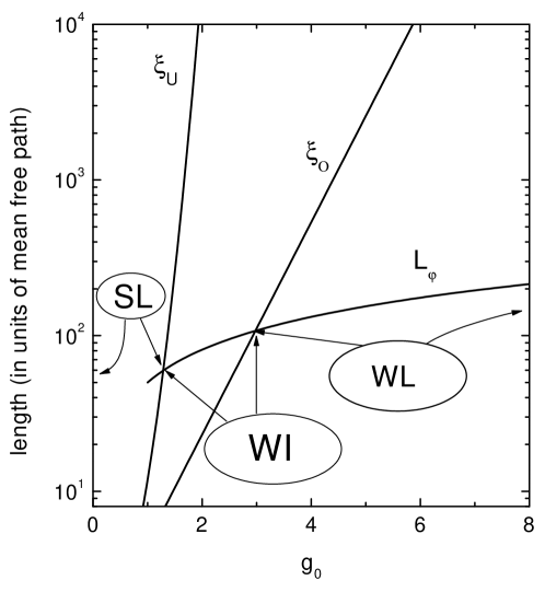
Figure 1: Schematic representation of the characteristic scale lengths $L_{\varphi}$, $\xi_{O}$, and $\xi_{U}$ plotted versus conductance $g_{0}\equiv k_{F}l$.

When the phase breaking length is much shorter than the localization lengths, $L_{\varphi}\ll\xi_{O},\,\xi_{U}$, the system is in the WL regime for an arbitrary magnetic field. In classically strong magnetic fields, the MR is produced by the interaction-induced Altshuler-Aronov correction to the conductivity (see Ref. GornyiMirlin, for review). At low magnetic fields, the negative MR, arising due to the suppression of quantum interference, is a well-known manifestation of weak localization Altshuler ; Hik ; AKhLL . This effect will be the subject of the present paper.

In Fig. 1, for values of $g_{0}$ lying to the left from the point of intersection of $\xi_{U}$ and $L_{\varphi}$ curves foot-Lvstau , the 2D system is in a strong localization (SL) regime. It is commonly believed that the transport in the SL case is of a hopping SE nature. The magnetoresistance in this regime is also related to the influence of magnetic field on the quantum interference and has been studied in Refs. spivak, ; Sarachik, ; Imry1, ; Imry2, . In particular, a parabolic low-field MR in the hopping regime was predicted. However, the results based on the conventional hopping picture cannot be directly applied to the experimental situation addressed in this paper, even when $\sigma(B=0)\lesssim G_{0}$. This is because the usual concepts of hopping (including the percolation treatment) are justified only when the disorder is large.

Finally, there is an intermediate regime which we term “weak insulator” (WI) regime, when the phase-breaking length $L_{\varphi}$ is between the $\xi_{U}$ and $\xi_{O}$ lines. In this regime electrons are localized at zero $B$ and the WL theory does not work. However, already a very weak magnetic field shifts the actual localization length $\xi(B)$ toward $\xi_{U}$ making $\xi(B)>L_{\varphi}.$ In such a situation the transport is again of the diffusive nature. Therefore, the theory of weak localization can be applied when the MR is considered for $\xi_{O}\ll L_{\varphi}\ll\xi(B)$, even though at zero $B$ the total conductance is smaller than unity. Obviously, this situation is only possible when $k_{F}l\gtrsim 1$. This is a necessary condition for opening a window between the two localization lengths $\xi_{O}$ and $\xi_{U}$. The WI-problem with a low conductance $g(T)<e^{2}/h$ at $B=0$ but with $g_{0}=k_{F}l>1$ should be therefore contrasted with the conventional SL problem with $k_{F}l\ll 1$ where the conductivity mechanism is the hopping. It is worth mentioning, however, that in three-dimensional systems near the mobility edge, a magnetic field also leads to the delocalization of electronic states (reentrance phenomenon), giving rise to a shift of the mobility edge, in a close similarity to the 2D WI regime 3DWI . Actually, the WI-regime has also much in common with the notion of a “moderate insulator”, introduced in Ref. gershenson-1D, to describe the crossover between the WL and SL regimes in quasi-one-dimensional semiconductor wires.

Generally speaking, at $k_{F}l\gtrsim 1$ the nature of transport of interacting electrons at very low $T$ (when the states are localized with large enough localization length $\xi_{O}\gg l$) is not fully understood. At microscopic scales, $l<L<\xi_{O},$ the electron dynamics is diffusive. The magnetic field serves as a probe of these scales and hence the MR can provide important information about the crossover between the localization and diffusion. The WL theory can be generalized (using, e.g., scaling arguments) to describe this crossover. Of course, the corrections of higher orders in $(k_{F}l)^{-1}$ become then important. Thus it is desirable to understand the role of these corrections in magnetotransport.

Apart from the scaling theory of Anderson localization, there is a self-consistent theory Woelfle ; Vollhardt-Woelfle , which enables to calculate the conductivity for arbitrary value of the quantum interference correction for $B=0$. However, as we will show below, while at zero $B$ the self-consistent theory works rather well, its generalization to the case of finite $B$ fails to describe correctly the magnetoconductivity (MC) (see Ref. Vollhardt-Woelfle, for discussion) in the crossover between the diffusive and localized regimes. In this paper we will concentrate on study of higher-order corrections to the conductivity using a systematic perturbation theory and scaling approach.

Experimentally, the low-field magnetoresistance in the range of intermediate conductances and in the crossover regime between the diffusion and localization in 2D systems has been studied in Refs. Pepper, ; Davies83, ; Hsu, ; Simmons00, ; proskur, ; brunthaler, ; WLtoSL, ; coleridge, ; pusep, ; krav, . It turns out that the MC even at low conductance, $\sigma(B=0)\lesssim G_{0}$, can be still fitted by the well-known weak-localization expression Hik ; AKhLL derived for $k_{F}l\gg 1$ (we will term it the WLMC-formula throughout the paper), but with a reduced prefactor $\alpha<1$ WLtoSL . Similar observations have been recently reported in Refs. pusep, ; krav, . In Refs. pusep, the magnetotransport has been studied in quasi-2D systems (doped GaAs/AlGaAs superlattices) and the MR has been shown to be generated by the quantum interference. A self-consistent theory of the MC has been employed to fit the data. In Ref. krav, , the MR in a weak perpendicular magnetic field was measured in the vicinity of an apparent metal-insulator transition AKS01 ; AMP01 in a $Si$ structure of $n$-type. In this experiment, the magnetoresistance on the metallic side was perfectly fitted by the WL formula with the prefactor $\alpha$ decreasing with lowering the density (i.e. upon approaching the transition). At the lowest density, the value $\alpha$ was reported krav to be $\sim 10$ times smaller than that obtained deeply in the metallic state. Finally, the authors of Ref. Hsu, , who measured the magnetoconductance in ultrathin metallic films, claimed that while for $\sigma(B=0)>G_{0}$ the MR is well described by the WL formula, for $\sigma(B=0)<G_{0}$ the MR corresponds to the hopping picture.

An important quantity extracted from the measured low-field MR is the phase breaking time $\tau_{\varphi}$, usually treated as a fitting parameter in the WLMC-formula. With the decreasing of the conductance, the corrections to this formula become more pronounced and thus the extracted value of $\tau_{\varphi}$ may strongly deviate from the true one. Therefore, there is a clear need for a systematic (both theoretical and experimental) analysis of the MR at decreasing conductance, including the crossover regime $\sigma(B=0)\sim G_{0}.$ A large scatter of experimental data on the phase breaking time which is evident even in the case $k_{F}l\gg 1$ renders reliable interpretation of the data at intermediate values of $k_{F}l$ difficult. Some of these reasons have been understood. These are the influence of $\delta$-doped layers Tau-phi , dynamical defects dyndef , and macroscopic inhomogeneities macro on the phase relaxation time, the temperature dependence of the mobility of electrons in quantum well due to temperature dependent disorder in the doped layers e-e , and the scattering on magnetic impurities VG . Nevertheless, the results obtained in Ref. WLtoSL, for both interference and electron-electron contributions to the conductivity in the range of not very high values of $g_{0}$ are (surprisingly) in a qualitative agreement with the existing theories of conductivity corrections, developed for high conductance. It was shown in Ref. WLtoSL, that at not very high values of $k_{F}l$ (at low electron densities), the role of the interaction correction to the conductivity becomes less important and the main effect comes from the interference. (This is because the interaction correction in the triplet channel Altshuler ; fink increases with decreasing $k_{F}$, and tends to cancel out the exchange contribution.) However, the experimental results have been interpreted in Ref. WLtoSL, only qualitatively.

In this paper we present the results of a quantitative analysis of the interference corrections to the conductivity and the negative MR at decreasing $k_{F}l$. We are not going to discuss a theory of the MR in the range $k_{F}l<1$ and $\sigma(B\neq 0)\ll G_{0},$ corresponding to the SL regime. On the other hand, we address, in particular, the WI regime, when the zero-B conductivity can be less than $G_{0}$ at low $T$.

The interpretation of experimental results obtained for 2D electron gas in GaAs/In_xGa_1-xAs/GaAs single quantum well structures is based on the theory taking into account terms of higher order in $(k_{F}l)^{-1}$. We show that the standard “one-loop” WL theory is adequate for $\sigma\gtrsim(10-20)\,G_{0}$. Calculating corrections of the next (“second-loop”) order, we expand the range of the quantitative agreement between the theory and experiments down to significantly lower conductivity of about $3\,G_{0}$. This is largely related to a fortunate circumstance that ${\cal O}(1/g^{3})$-terms are absent in the perturbative expansion of beta-functions governing the scaling of the conductance Hik81 . Therefore, the corrections to the second-loop expressions derived in this paper are proportional to $(G_{0}/\sigma)^{2}$ and hence turn out to be numerically small at such values of the conductivity foot-nonpert .

We demonstrate that the WLMC-formula can be still used to fit the MR in the crossover from the WL and WI regimes. It is shown that the main effect of higher-order terms is a reduction of the prefactor $\alpha$ in the these formulas,

$$\alpha\simeq 1-\frac{2G_{0}}{\sigma}.$$ (4)

This expression appears to be applicable for $\alpha\gtrsim 0.3,$ when the fitting procedure is carried out in a broad range of magnetic fields. Thus, it becomes possible to experimentally determine the phase breaking time within a wide conductivity range, $\sigma\simeq(3-60)G_{0}$. Moreover, the qualitative agreement between the experimental data and the (properly modified) WL theory persists down to significantly smaller zero-$B$ conductivity $\sigma(T,B=0)\lesssim G_{0}$, provided that $k_{F}l>1$. In other words, one of the main results of this paper is that the theory of quantum corrections to the conductivity works rather well at the limit of its applicability, i.e. even for “intermediate” values of $g$ of order of unity, down to $\sigma\sim e^{2}/h$.

We also show that when applied to the MC in the WI regime, $\xi_{O}<L_{\varphi}<\xi_{U}$, the fitting procedure based on the conventional WLMC-formula, yields the value of the dephasing rate which deviates from the real one and contains information about the localization length, $\xi_{O}.$ This observation may be relevant to the explanation of the tendency to a low-$T$ saturation of the experimentally extracted dephasing time reported recently in Refs. proskur, ; brunthaler, , where WL was studied at intermediate conductances in the vicinity of the apparent metal-insulator transition.

The paper is organized as follows. The next three sections are devoted to a theoretical consideration of the problem of the dephasing and quantum corrections to the conductivity. In Section II, we recall the basic theoretical results on the dephasing, interference correction, and interference induced negative MR. Primary emphasis is put on the possible reasons of the above mentioned fact that the low-field negative MR is practically always well described by the WLMC-expression with the reduced prefactor $\alpha$. In Section III we take a close look at the interaction correction in the Cooper channel, which is most frequently invoked for the explanation of the reduction of $\alpha$. The theory of interference quantum corrections developed in the next order in $1/g$ is expounded in Section IV. The experimental results and their analysis are presented in Sections V and VI . Finally, Section VII is devoted to the conclusions.

II Dephasing, interference correction, and magnetoconductivity

II.1 Dephasing time in zero magnetic field

Let us start with the consideration of WL effects in zero magnetic field at large values of the conductance, $g\gg 1$ (here the conductance is measured in units of $\pi G_{0}$). This condition allows one to treat the dynamics of a particle quasiclassically, relating the conductivity correction to the return probability. Within the framework of the conventional theory of the WL developed in the first order in $1/g$, the interference quantum correction in a 2D system is given by Altshuler ; AAKL-MIR ; LeeRam ; aleiner ; GorkovLarkinKhmelnitskii

$$\frac{\delta\sigma}{G_{0}}=-\ln\left(\frac{\tau_{\varphi}}{\tau}\right).$$ (5)

This result holds within the diffusion approximation, justified for $\tau_{\varphi}/\tau\gg 1$. In this paper, we will restrict ourselves to the diffusive regime [$\tau_{\varphi},\hbar/(k_{B}T)\gg\tau$] and will not consider the ballistic contribution.

In the WL theory, the phase breaking (also known as phase relaxation, dephasing, or decoherence) time $\tau_{\varphi}$ is a characteristic time scale at which the two waves traversing along the same path in opposite directions lose their relative phase coherence due to inelastic scattering events. At longer times (or trajectories’ lengths) the two waves do not interfere and therefore do not contribute to the WL correction to the conductivity. At low temperatures the main source of the inelastic scattering is the Coulomb electron–electron (e-e) interaction. In this paper, we will not address the contribution of other decoherence mechanisms such as electron–phonon interactions, scattering on dynamical defects, interaction with magnetic impurities, etc. Generally, the phase relaxation time is different from other inelastic scattering times, e.g. the energy-relaxation time AAK82 ; Altshuler ; Aleiner2002 . Moreover, the phase relaxation may depend on the geometry of the system. In particular, the damping of Aharonov-Bohm oscillations in quasi-one-dimensional rings differs ludwig-mirlin from the phase relaxation rate found for infinite wires AAK82 . It is worth mentioning, however, that the same conventional WL phase relaxation time governs the temperature behavior of mesoscopic conductance fluctuations Aleiner2002 and the (two-loop) WL correction in the unitary ensemble polyakov-samokhin .

The phase breaking rate $\tau_{\varphi}^{-1}$ can be calculated using the path-integral approach and/or perturbative diagrammatics Altshuler ; AAK82 ; Eiler ; aleiner ; Aleiner2002 . As was shown in Ref. AAK82, , the inelastic scattering events with energy transfer smaller than $\hbar/\tau_{\varphi}$ (corresponding to the phase breaking rate itself) do not give rise to the decoherence. Therefore, the dephasing rate can be found from the following self-consistent equation AAK82

$$\frac{1}{\tau_{\varphi}}=\frac{k_{B}T}{\hbar\,g}\ln\frac{k_{B}T\tau_{\varphi}}{\hbar}.$$ (6)

The solution of this equation is shown in Fig. 2 by the solid line. The product $T\tau_{\varphi}$ saturates with decreasing $g$ and monotonically increases with increasing the conductance. For the illustration purpose, in this figure we have also presented a formal solution of Eq. (6) at $g<1$ (dashed line), where the equation for the dephasing rate is no longer justified. The behavior (and even the meaning) of $\tau_{\varphi}$ for $g<1$ is a subtle issue and depends on the problem considered. In principle, when the actual conductance is not very high, the two equations, one for the conductivity and another for the phase-breaking time, are coupled and should be solved simultaneously.

In practice, one obtains the value of $\tau_{\varphi}$ from Eq. (6) using the iteration procedure. By iteration, starting with $\tau_{\varphi}^{(0)}=g\,\hbar/(k_{B}T),$ one obtains

$$\frac{1}{\tau_{\varphi}^{(1)}}=\frac{k_{B}T}{\hbar\,g}\ln g\ ,$$ (7)

and so on. Usually (for $g\gg 1$) one supposes that this iteration is sufficient for the quantitative description of the conductivity corrections. However, as seen from Fig. 2 it gives fully incorrect behavior of $\tau_{\varphi}$ below $g\simeq 5$, where one expects the dephasing time to approach the value $\sim 1/T$ at $g\sim 1$ for the case of Coulomb interaction. In the above consideration the value of the phase breaking time depends only on the conductivity and does not depend on other material parameters. In this sense, $\tau_{\varphi}$ shows the universal behavior.

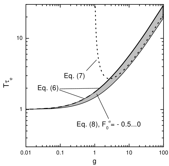
Figure 2: The conductivity dependence of $T\tau_{\varphi}$. Solid line is the solution of Eq. (6) (which coincides with Eq. (8) with $F_{0}^{\sigma}=0$), dotted line is the first iteration Eq. (7) for Eq. (6). The formal solution of Eq. (6) for $g<1$ is shown by the dashed curve. Shadow area represents the solutions of Eq. (8) found numerically for different values of $F_{0}^{\sigma}$ from the range $-0.5...0$. We set $k_{B}=\hbar=1$ here.

Recently, the dephasing time has been theoretically studied at arbitrary relation between temperature and elastic mean free time and taking into account the Fermi-liquid renormalization of the triplet channel of Coulomb interaction Aleiner379 . It has been shown that in the diffusive regime ($k_{B}T\tau/\hbar\ll 1$) the equation for $\tau_{\varphi}$ is analogous to Eq. (6):

$$\frac{1}{\tau_{\varphi}}=\left[1+\frac{3(F_{0}^{\sigma})^{2}}{(1+F_{0}^{\sigma})(2+F_{0}^{\sigma})}\right]\frac{k_{B}T}{\hbar\,g}\ln\frac{k_{B}T\tau_{\varphi}}{\hbar}.$$ (8)

The only difference in this equation is a factor on the right-hand side, which depends on the Fermi liquid constant $F_{0}^{\sigma}$. The value of $F_{0}^{\sigma}$ can be experimentally obtained from measuring the logarithmic (Altshuler-Aronov) quantum correction to the conductivity $\delta\sigma^{ee},$ caused by the e-e interaction Altshuler ; Finkelstein ; ZNA ,

$$\frac{\delta\sigma^{ee}}{G_{0}}=\left[1+3\left(1-\frac{\ln(1+F_{0}^{\sigma})}{F_{0}^{\sigma}}\right)\right]\ln\frac{k_{B}T\tau}{\hbar}=K_{ee}\ln\frac{k_{B}T\tau}{\hbar}.$$ (9)

In semiconductor structures, the value of $F_{0}^{\sigma}$ typically lies within the range from $-0.5$ to $0$ (for discussion see e.g. Ref. sav ; sav1 ). For the samples investigated here, $F_{0}^{\sigma}=-0.45...-0.25$, depending on the electron density ourKee . To show the difference between Eq. (6) and Eq. (8) we have plotted the dependences $\tau_{\varphi}(\sigma)$ for several $F_{0}^{\sigma}$ values in Fig. 2. It is seen that the difference increases with conductivity increase, but even for $g=100$ it does not exceed 30 %.

II.2 Negative magnetoresistance and dephasing time in magnetic field

How can the dephasing time be obtained experimentally? As a rule, the value of $\tau_{\varphi}$ (or the ratio $\tau/\tau_{\varphi}$ referred further as $\gamma$) is extracted from an analysis of the negative magnetoresistance arising due to the suppression of the WL by a transverse magnetic field. Practically in all the cases the experimental $\Delta\sigma(B)$-vs-$B$ curves are fitted to the well-known expression Hik ; Schm for the WL-magnetoconductivity (WLMC-expression):

$$\frac{\Delta\sigma(B)}{G_{0}} = \alpha\left\{\psi\left(\frac{1}{2}+\frac{1}{\tau_{\varphi}}\frac{\hbar}{4DeB}\right)-\psi\left(\frac{1}{2}+\frac{1}{\tau}\frac{\hbar}{4DeB}\right)-\ln\left(\frac{\tau}{\tau_{\varphi}}\right)\right\}$$ (10a)

$$\equiv \alpha{\cal H}(b,\gamma).$$ (10b)

Here

$$\Delta\sigma(B)=1/\rho_{xx}(B)-1/\rho_{xx}(0),$$ (11)

$\psi(x)$ is digamma function, $b=B/B_{tr}$, where $B_{tr}=\hbar/(2el^{2})=\hbar/(2ev_{F}^{2}\tau^{2})$, and $D=v_{F}^{2}\tau/2$. In what follows, we will consistently use the notations $\Delta\sigma$ for the magnetoconductivity and $\delta\sigma$ for conductivity corrections.

In the diffusive with respect to the magnetic field regime, $4DeB/\hbar\equiv\Omega_{B}\ll 1/\tau,$ one can use the asymptotics of the second digamma function, $\psi(1/2+1/\Omega_{B}\tau)\sim-\ln(\Omega_{B}\tau)$. Then the MR Eq. (10) can be rewritten as a function of a single parameter $\Omega_{B}\tau_{\varphi},$

$$\frac{\Delta\sigma(B)}{G_{0}}=\alpha\left\{\psi\left(\frac{1}{2}+\frac{1}{\Omega_{B}\tau_{\varphi}}\right)+\ln\left(\Omega_{B}\tau_{\varphi}\right)\right\}\equiv\alpha Y(\Omega_{B}\tau_{\varphi})$$ (12)

with the following asymptotics Altshuler ; Aleiner379 :

$$Y(x) = {x^{2}\over 24},\qquad\qquad\qquad\quad\quad x\to 0,$$ (13)

$$Y(x) = \ln\ x+\psi(1/2)+{\pi^{2}\over 2x},\quad 1\ll x\ll 1/\gamma,$$ (14)

where $\psi(1/2)=-2\ln 2-{\bf C}$ and ${\bf C}=0.5772..$ is the Euler constant. Also, using Eq. (10a) one can see that $\Delta\sigma(B)$ saturates at $b\gtrsim 1$. The precise way of saturation of $\Delta\sigma(B)$ depends on the character of the disorder. In principle, the value of the dephasing time can be obtained from the curvature of the parabolic MC in the limit of vanishing magnetic field, $B\to 0,$ see Eq. (13). However, usually the whole MC curve is fitted by the WLMC-formula Eq. (10) in the range of magnetic fields where the MC is logarithmic-in-$B$ and hence we will mainly consider the MC at $\Omega_{B}\tau_{\varphi}>1$ in this paper.

It is worth mentioning, that the WLMC-formula Eq. (10) was derived under the assumption that the magnetic field is classically weak and thus does not lead to a strong Drude-Boltzmann magnetoconductance caused by the bending of the cyclotron trajectories. This is justified by the condition $\omega_{c}\tau\ll 1,$ where $\omega_{c}$ is the cyclotron frequency. For high conductances, $g\gg 1$, the logarithmic interference-induced MC is already destroyed at much weaker magnetic fields, $b\sim 1$, which corresponds to $\omega_{c}\tau\sim 1/g\ll 1$. Therefore, for $g\gg 1$ one can use the relation (11). However, when the conductance is not too high, $g\sim 1$, which is the case addressed below, the two conditions $b=1$ and $\omega_{c}\tau\sim 1,$ coincide. Then the bending of particles’ trajectories may become noticeable already in the WL-range of magnetic fields. We recall, however, that the bending of trajectories does not give rise to the magnetoresistance, while the destruction of the interference does. This is related to the fact that the interference correction stems from the ($B$-dependent) correction to the impurity scattering cross-section foot-time ; dmit ; Groshev and hence renormalizes the value of the elastic scattering rate, $1/\tau$. This is nothing but the renormalization of the longitudinal resistivity, so that the MR arises due to the $B$-dependence of the effective transport scattering time. This also explains why WL effects do not give rise to the correction to the Hall resistivity, $\rho_{xy}$: the Drude-Boltzmann expression for $\rho_{xy}$ merely does not contain $\tau$. In other words, Eq. (10) is in fact the correction to the MR Groshev and as such is actually applicable directly to the MR curves obtained in the experiment (without inverting the resistivity tensor), even when the classical effect of the magnetic field becomes visible for $g\sim 1$ at $b\lesssim 1$.

Although the prefactor $\alpha$ has to be equal to unity within the framework of the conventional weak-localization theory, it is always used by experimentalists as the second fitting parameter together with $\tau_{\varphi}$. An important point is that almost all experimental data are better fitted with $\alpha<1$, contradicting the theory. In order to feel certain of that one obtains the true value of $\tau_{\phi}$ in such a situation, it is necessary to understand the reasons for the lowering of the prefactor in each specific case. Possible sources for this discrepancy have been discussed in the literature since the discovery of weak localization. They are listed below with relevant comments.

1. Interband scattering. It can change the value of $\alpha$ depending on the rate of interband transitions Altshuler . The most frequently used systems where this effect is important are $Si$-based structures of $n$-type conductivity, where there are several valleys in the spectrum. This mechanism is not active in our case. We will address the $n$-InGaAs quantum wells with simplest single-valley spectrum and only one subband of the size quantization occupied.

2. Effect of ballistic paths. Strictly speaking, Eq. (10) was derived within the diffusion approximation. The contributions of short trajectories, $L\lesssim l$, are treated incorrectly (even for weak magnetic fields, $B<B_{tr}$). Therefore, Eq. (10) is only valid under the conditions: $\tau/\tau_{\varphi}\ll 1$ and $b\ll 1$. Beyond the diffusion approximation the MC was analyzed in a number of papers, Refs. zyuzin, ; kavabata, ; Schm, ; dyak, ; cassam, ; dmit, ; Groshev, ; our1, . The analytical expressions obtained therein are quite cumbersome and not easy-to-use for analysis of experimental data, while the high-field asymptotics $\delta\sigma(B)\propto 1/\sqrt{B}$ is reached only at very strong magnetic fields, $B\gg B_{tr}$. Note that in many papers kavabata ; Schm ; dyak the contribution of non-backscattering processes (important in the ballistic limit zyuzin ; dmit , see also Appendix C) was overlooked.

   The applicability of Eq. (10) (with the second digamma function not replaced by its “diffusive” asymptotics) beyond the diffusion regime has been analyzed in Ref. our1, where it has been used to fit the results of numerical simulation (treating the numerical results like experimental data). It has been shown that if the range of magnetic fields where the MC is fitted using Eq. (10) includes also strong fields $B\gtrsim B_{tr}$ [where Eq. (10) is formally no longer justified], the resulting value of $\alpha$ will be less than unity. Nevertheless, the value of $\tau_{\varphi}$ obtained in this way happens to be close to the true one. A situation where ballistic contribution is relevant occurs frequently in very high-mobility structures where $B_{tr}$ is very low and can be as small as $10^{-3}..10^{-4}$ Tesla. In what follows we will address only the case of weak magnetic fields $B<B_{tr}$ and low temperatures, $\tau_{\varphi}\gg\tau$.

3. Spin relaxation. In quantum wells with inversion asymmetry, the Rashba or/and Dresselhaus mechanisms of spin-orbit splitting of the energy spectrum lead to spin relaxation which suppresses the interference–induced negative magnetoresistance in very low magnetic fields and results in a positive MR. If this effect is not so strong to induce the positive MR ($\tau_{\rm so}\gg\tau_{\varphi}$ where $\tau_{\rm so}$ is the spin-orbit relaxation time), it can nevertheless distort the shape of MR curve in vicinity of $B=0$ and, thus, change the parameter $\alpha$ if the data are treated with the help of Eq. (10). Our analysis shows that the parameters of the best fit are unstable in this case. In particular, the value of the prefactor strongly depends on the range of magnetic field, in which the fit is carried out, and it is always greater than unity. This implies that one has to exercise caution, when fitting the MC by Eq. (10a) if even a weak spin-orbit interaction is present in the system. The role of spin effects in the WL was considered for the first time in Ref. Hik, . Using a generalized Hikami-Larkin-Nagaoka formula Hik , including the spin effects, one should obtain the value of the prefactor as given in Ref. Hik, . Effects of spin-orbit interaction on the WL (which are especially important in hole systems) were further considered in more recent papers, both theoretically and experimentally (see e.g. Refs. pikus, ; Malshukov, ; knapandco, ; zduniak, ; GDK, ; Golub, ; Studen, and references therein).

4. Magnetic field impact on the dephasing. The expression Eq. (10) was derived under the assumption that the dephasing rate does not depend on magnetic field. As shown in Refs. aleiner, ; Eiler, ; AAA85, ; Aleiner379, , the magnetic field (rendering the inelastic processes with low energy transfer to be inefficient) leads effectively to a decrease of the dephasing rate. To our knowledge this effect is always ignored in experimental papers. In Ref. tauphiB, we have analyzed this effect both analytically and numerically. The magnetoconductance can be described by Eq. (10) with a certain $B$-dependent phase-breaking time $\tau_{\varphi}(B)$ in the first digamma function Aleiner379 in the whole range of magnetic fields $b\lesssim 1$ (including the crossover region $\Omega_{B}\sim 1/\tau_{\varphi}$, not addressed accurately in Ref. Aleiner379, ). Effect of the magnetic field on the phase breaking rate makes the negative magnetoresistance smoother in shape and lower in magnitude than that found with the constant phase breaking rate. Nevertheless our analysis tauphiB shows that the $\Delta\sigma$-versus-$B$ plot can be well fitted by the standard expression Eq. (10) with $\alpha\neq 1$ and a constant $\tau_{\varphi}$. The fitting procedure gives the value of $\tau/\tau_{\varphi}$ which is close to the value of $\tau/\tau_{\varphi}(B=0)$ with an accuracy of $25$% or better when $k_{F}l\gtrsim 3$ and the temperature varies within the range from $0.4$ to $10$ K, for electron concentrations considered in this paper.

5. Electron-electron interaction in the Cooper channel. In low magnetic field the two interaction-induced terms can contribute to the magnetoresistance Altshuler ; AAKL-MIR ; altshulerMT . The first one, known as the Maki-Thompson correction Larkin80 ; MakiT , has at $\Omega_{B}\ll T$ just the same $B$-dependence as the expression Eq. (12) but with the negative prefactor. Its value depends on the absolute value of the effective constant of interaction in the Cooper channel, $\lambda_{c}(T)$. The second term is related to the correction to the density of states (DoS) due to the interaction in the Cooper channel altshulerMT and can be positive or negative depending on the sign of $\lambda_{c}(T)$, which depends, in its turn, on the sign of the effective interaction between electrons. The DoS-correction becomes important at stronger magnetic fields $\Omega_{B}\gg T$, where it overcomes the Maki-Thompson correction. The role of this interaction in our experimental situation will be considered in Sections III and V.2.2. It will be shown that it is not the effect of interaction in the Cooper channel that determines the strong decrease of the prefactor $\alpha$ in the heterostructures investigated at not very high conductance.

6. Corrections of higher orders in $1/g$. The formula Eq. (10) is the first-order in $1/g$ correction to the conductivity and therefore is valid only for large conductances. Of course, there are corrections of higher orders in $1/g$ which become important with the increase of the disorder strength or with decreasing electron concentration. We analyze the higher-order terms, both in the WL contribution and in the correction induced by the mutual effect of WL and the Coulomb interaction aleiner , in Section IV.1 and Section IV.2. This consideration allows us to find the ${\cal O}(1/g)$-corrections to the prefactor $\alpha$ and to understand also the relation between the experimentally extracted value of $\gamma$ and the true phase-breaking time $\tau_{\varphi}$ at $\sigma(B=0)\lesssim G_{0}$.

In what follows, we will concentrate on the last two effects which we believe are the most relevant sources of the reduction of the prefactor in WLMC-expression, Eq. (10). We will show that at not very high conductance, the effect of corrections of higher orders in $1/g$ is more important than the effect of the electron-electron interaction in the Cooper channel.

III Interaction corrections in the Cooper channel

It is commonly believed that it is the interaction correction in the Cooper channel (mainly the Maki-Thompson correction to the conductivity MakiT ; Larkin80 ) which determines the reduction of the prefactor in the MC. Indeed, in low magnetic fields the two terms induced by the interaction in a Cooper channel contribute to the magnetoconductance Altshuler ; AAKL-MIR ; altshulerMT

$$\Delta\sigma^{\rm C}_{ee}=\Delta\sigma^{\rm MT}+\Delta\sigma^{\rm DoS},$$ (15)

where $\Delta\sigma^{\rm MT}$ is the Maki-Thompson correction to the conductivity Larkin80 and $\Delta\sigma^{\rm DoS}$ arises due to the correction to the DoS induced by the interaction in the Cooper channel Alt-Varlamov ; foot-AL .

At $B=0$ and high conductance $g\gg 1,$ for a repulsive interaction these corrections read Larkin80 ; Altshuler ; AAKL-MIR ; Alt-Varlamov (in what follows we set for brevity $k_{B}=\hbar=1$)

$$\delta\sigma^{\rm MT}=G_{0}\frac{\pi^{2}\lambda_{c}^{2}(T)}{6}\ln(T\tau_{\varphi})=G_{0}\frac{\pi^{2}}{6\ln^{2}(T_{c}/T)}\ln(T\tau_{\varphi}),$$ (16)

and

$$\delta\sigma^{\rm DoS}=-G_{0}\ln[\lambda_{c}(T)\ln(T_{c}\tau)]=-G_{0}\ln\left[\frac{\ln(T_{c}\tau)}{\ln(T_{c}/T)}\right].$$ (17)

An important quantity governing the strength of the corrections Eqs. (15), (16), and (17) is the effective amplitude of the interaction in the Cooper channel,

$$\lambda_{c}(T)=\left[\frac{1}{\lambda_{0}}+\ln\frac{2\eta}{\pi T}+{\bf C}\right]^{-1}\equiv\frac{1}{\ln(T_{c}/T)},$$ (18)

where $\lambda_{0}$ is the dimensionless “bare” interaction constant, $\eta$ is the Fermi energy for Coulomb repulsion ($\lambda_{0}>0$) between electrons. (In the case of a phonon-mediated attraction, $\lambda_{0}<0$, $\eta$ is given by the Debye frequency. varlamov-larkin ) Thus we have for the case of the Coulomb repulsion (see also Ref. varlamov-larkin, for the case of attraction)

$$T_{c}\simeq\frac{2E_{F}e^{\bf C}}{\pi}\exp(1/\lambda_{0})>E_{F}.$$ (19)

Similarly to the WL correction, the above corrections stem from the interference of time-reversed paths and therefore are affected by the magnetic field. However, since the interaction is also involved in these corrections, an additional parameter $\Omega_{B}/T$, relating the magnetic field and the temperature, appears. This should be contrasted with the WL correction, in which only the parameters $\Omega_{B}\tau_{\varphi}$ and $\Omega_{B}\tau$ play an important role.

For $\Omega_{B}\ll T,$ the Maki-Thompson correction to the MC is given by Larkin80 ; altshulerMT ; Altshuler (see also Appendix A)

$$\Delta\sigma^{\rm MT}\equiv\delta\sigma^{\rm MT}(B)-\delta\sigma^{\rm MT}(0)=-G_{0}\frac{\pi^{2}}{6\ln^{2}(T_{c}/T)}Y(\Omega_{B}\tau_{\varphi}),$$ (20)

where $Y(x)$ is just the same function [defined in Eq. (12)] that describes the MC due to the suppression of WL. Thus the Maki-Thompson correction gives rise to a parabolic MC at $\Omega_{B}\ll 1/\tau_{\varphi}$ and to a logarithmic MC at $1/\tau_{\varphi}\ll\Omega_{B}\ll T$. In the same range of magnetic fields, $\Omega_{B}\ll T$, the DoS-correction yields a parabolic MC altshulerMT ; AAKL-MIR

$$\Delta\sigma^{\rm DoS}=-G_{0}\lambda_{c}(T)\varphi_{2}(\Omega_{B}/2\pi T),$$ (21)

where the function $\varphi_{2}(x)$ is given by, altshulerMT

$$\varphi_{2}(x)=\int_{0}^{\infty}dt\frac{t}{{\rm sinh}^{2}t}\left[1-\frac{xt}{{\rm sinh}(xt)}\right]=\left\{\begin{array}[]{ll}\zeta(3)x^{2}/4,&\quad x\ll 1,\\ \ln x,&\quad x\gg 1,\end{array}\right.$$ (22)

with $\zeta(x)$ [$\zeta(3)=1.202..$] the Riemann zeta-function. Comparing Eqs. (20) and (21), we find that for $1/\tau_{\varphi}\ll\Omega_{B}\ll 2\pi T\times{\rm min}\{1,[\lambda_{c}(T)\ln(T\tau_{\varphi})]^{1/2}\}\sim T$ the logarithmic-in-$B$ Maki-Thompson correction to the MC dominates over the DoS-correction.foot-MTBto0 The Maki-Thompson correction has the same $B$-dependence as the interference correction and effectively reduces the total prefactor in the MC.Larkin80 The temperature dependence of $\lambda_{c}(T)$ translates into the $T$-dependence of the effective prefactor $\alpha<1$ in Eq. (12).

Let us consider these corrections at stronger magnetic fields. Unfortunately, the exact crossover functions appear to be rather cumbersome Altshuler ; AAKL-MIR and we will restrict ourselves to the analysis of the asymptotic forms of the corrections at $\Omega_{B}\gg T$. As shown in Appendix A, the Maki-Thompson contribution to the MC saturates in this range of magnetic fields. On the other hand, it turns out that Eq. (21) works there as well, yielding a dominating logarithmic-in-$B$ contribution AAKL-MIR ; altshulerMT

$$\Delta\sigma^{\rm DoS}=-G_{0}\frac{\ln(\Omega_{B}/2\pi T)}{\ln(T_{c}/T)}.$$ (23)

This result can be also obtained if for the calculation of $\delta\sigma^{\rm DoS}(B)$ at $\Omega_{B}\gg 2\pi T,$ one simply substitutes $\Omega_{B}/2\pi$ instead of $T$ in Eq. (17), thus taking into account the $B$-dependence of the effective coupling constant, which gives

$$\frac{\Delta\sigma^{\rm DoS}(B)}{G_{0}}=\frac{\delta\sigma^{\rm DoS}(B)-\delta\sigma^{\rm DoS}(0)}{G_{0}}\simeq-\ln\left[{\ln(T_{c}/T)\over\ln(2\pi T_{c}/\Omega_{B})}\right]\simeq-{\ln(\Omega_{B}/2\pi T)\over\ln(T_{c}/T)}.$$ (24)

We thus see that the interaction corrections in the Cooper channel indeed reduce the effective prefactor $\alpha$ in the MC, as compared to the non-interacting case:

$$\alpha^{C}_{\rm ee} = 1-{\pi^{2}\over 6\ln^{2}(T_{c}/T)},\quad\Omega_{B}\ll T,$$ (25)

$$\alpha^{C}_{\rm ee} = 1-{1\over\ln(T_{c}/T)},\qquad\Omega_{B}\gg T.$$ (26)

Here only the asymptotics of the prefactor is presented (and we write the corresponding conditions with the logarithmic accuracy). To describe the crossover, one can use Eqs. (21) and (22) for the DoS-correction, and Eq. (68) for the Maki-Thompson one, in the whole range of magnetic fields.

When the conductance is not very high (which is the situation of a primary interest to us in Section V), $\hbar/\tau_{\varphi}\to k_{B}T$ with decreasing $g$ (see Fig. 2), so that both corrections are quadratic in $B$ for $\Omega_{B}\ll T$. Therefore the reduction of the prefactor in the nontrivial logarithmic MC occurring at $\Omega_{B}\gg 1/\tau_{\varphi}$ is determined by the DoS-correction and given by Eq. (26) in this case.

Let us now estimate the values of the prefactor $\alpha^{C}_{\rm ee}$ corresponding to the typical parameters of our experiment. Since we consider here the Coulomb repulsion, we have $\eta\simeq E_{F}$. We also set $\lambda_{0}$ to be of the order of $|F_{0}^{\sigma}|$ for our estimates. All the data presented below are obtained for electron density that changes from approximately $1\times 10^{16}$ m^-2 ($E_{F}\simeq 450$ K) to $2\times 10^{15}$ m^-2 ($E_{F}\simeq 90$ K), the value of $F_{0}^{\sigma}$ varies from $-0.25$ to $-0.45$.ourKee Equation  (19) gives the following estimate for $T_{c}$: it is $3\times 10^{4}$ K for the highest electron density and $10^{3}$ K for the lowest one. Substituting these quantities in Eq. (26) we see that the value of $\alpha^{C}_{\rm ee}$ is only slightly less than unity for any electron density and temperature in the range $(0.4-4.2)$ K: its maximal value, $\alpha^{C}_{\rm ee}\simeq 0.99$, corresponds to $n=10^{16}$ m^-2, $T=0.4$ K, and $\Omega_{B}\ll 2\pi T$, the minimal value, $\alpha^{C}_{\rm ee}\simeq 0.85$, is realized for $n=2\times 10^{15}$ m^-2, $T=4.2$ K, and $\Omega_{B}\gg 2\pi T$. For reference, the experimentally observed decrease of the prefactor is about five times as large (see Section V). The contributions of the corrections in the Cooper channel and WL-contribution in the magnetoconductivity are illustrated by Fig. 3. For calculation, we have used the parameters of one of the samples investigated in Section V: $k_{F}l=2.2$, $E_{F}=11$ meV, and $T=1.5$ K. It is clearly seen that the corrections in the Cooper channel only slightly reduce the magnetoconductivity in magnitude and practically does not change the curve shape. The last is more evident if one applies the standard fitting procedure trying to describe the total correction $\Delta\sigma^{\rm WL}+\Delta\sigma^{\rm MT}+\Delta\sigma^{\rm DoS}$ by Eq. (10) (compare circles and dashed line in Fig. 3). This procedure demonstrates once again that the interaction in the Cooper channel cannot be responsible for the reduction of the prefactor in the magnetoconductivity: in this example the interaction correction results in reduction of $\alpha$ on the value $0.15$ instead of $0.65$ observed experimentally.

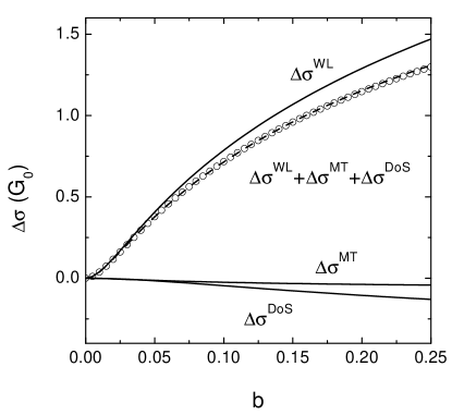
Figure 3: The contributions to the magnetoconductivity in the Cooper channel as compared with that due to the weak localization. The $\Delta\sigma^{WL}$-versus-$b$ curve is Eq. (10) with $\alpha=1$, $\Delta\sigma^{MT}$-versus-$b$ curve is calculated from Eqs. (21) and (22), $\Delta\sigma^{MT}$-versus-$b$ curve is Eq. (68). The parameters corresponding to the case of $k_{F}l=2.2$ (see Section V for experimental details) have been used in the calculations: $E_{F}=11$ meV that corresponds to $n\simeq 2.8\times 10^{15}$ m^-2, $F_{0}^{\sigma}=-0.42$, ourKee $\tau=6.2\times 10^{-14}$ s, $\gamma^{-1}=104$, $T=1.5$ K. Circles are the sum of all the contributions, dashed line is the best fit by Eq. (10), which gives $\alpha=0.85$, $\gamma^{-1}=113$. Note, the prefactor value obtained experimentally is $0.35$ (see Fig. 7 and Table 1).

In what follows we will consider the conductivity corrections of higher-order in $1/g$. Taking into account such terms, we will find the ${\cal O}(1/g)$-correction to the prefactor $\alpha$. Therefore, in order to determine the main source of the reduction of $\alpha$ one should compare the values of $G_{0}/\sigma$ and $\lambda_{c}(T)$. It turns out that already at sufficiently high values of $\sigma\sim 10G_{0}$ the $1/g$-corrections win. Moreover, from the theoretical point of view, the latter mechanism of reduction of $\alpha$ will always win in the limit $T\to 0$, since $\lambda_{c}(T)$ decreases while $1/g(T)$ increases with decreasing $T$.

IV Higher-order corrections to the magnetoconductivity

IV.1 Second-loop correction to the magnetoconductivity: interference term

At intermediate and small values of $k_{F}l$ the higher order corrections in $1/g$ should be taken into account. To sum up these corrections, a self-consistent theory of Anderson localization was invented in Ref. Woelfle, . The generalization of this approach onto the case of finite magnetic field was developed in Ref. Bryksin, (see also earlier works, Refs. Ioshioka, ; Ting, ). However, as will be seen below, there is no agreement between the theory Bryksin and experimental results at low conductivity. This is related to the fact that the self-consistent theory Bryksin mistreats the quantum corrections involving diffusons, as was pointed out in Ref. Vollhardt-Woelfle, .

Another approach is based on the systematic analysis of higher-order quantum corrections arising from the second-loop term in scaling theory of localization.GorkovLarkinKhmelnitskii ; gang4 Physically, the second-loop corrections correspond to the contributions of the interfering waves traversing along the paths that form two loops (instead of a single loop for the first-order WL correction) in the real space. We start with the analysis of the next order correction for non-interacting electrons.GorkovLarkinKhmelnitskii It is well known LeeRam ; Hik81 ; wegner ; brezin ; Efetov that the $\beta$-function,

$$\beta({\mathsf{g}})={\partial\ln{\mathsf{g}}\over\partial\ln L},$$ (27)

governing the scaling of the conductance with the system size $L,$ depends on whether the magnetic field is present (unitary ensemble) or absent (orthogonal ensemble). Note that in this section, we measure the conductance per spin in units of $G_{0}$, which allows us to avoid the appearance of additional factors of $\pi$; we will use a notation ${\mathsf{g}}\equiv\pi g/2$ for the such defined dimensionless conductance. At large conductance, only the first non-vanishing order of the expansion of $\beta({\mathsf{g}})$ in powers of $1/{\mathsf{g}}$ is relevant. Of course, the renormalization group equation perturbative in $1/{\mathsf{g}}$ can not be applied to the region of ${\mathsf{g}}\lesssim 1$.

Let us discuss the crossover between the orthogonal and unitary ensembles. In the unitary ensemble the one-loop (Cooperon) term in beta-function vanishes, and the $\beta$-function is given for ${\mathsf{g}}\gg 1$ by wegner ; Hik81 ; brezin

$$\beta_{U}({\mathsf{g}})=-{1\over 2{\mathsf{g}}^{2}}+{\cal{O}}\left({1\over{\mathsf{g}}^{4}}\right).$$ (28)

Solving the scaling equation Eq. (27) with Eq. (28), one gets for $L\ll\xi_{U},$ i.e., for ${\mathsf{g}}\gg 1$.

$${\mathsf{g}}={\mathsf{g}}_{0}-{1\over 2{\mathsf{g}}_{0}}\ln(L/l),$$ (29)

where ${\mathsf{g}}_{0}=\pi k_{F}l/2$. The conductivity (in the spin-degenerate system) is then given by

$$\sigma=2G_{0}{\mathsf{g}}=\sigma_{0}-{e^{2}\over 2\pi^{2}\hbar}{1\over\pi k_{F}l}\ln\left(\tau^{D}_{\varphi}/\tau\right).$$ (30)

Here we use the phase-breaking length as the cutoff for the renormalized conductance, $L=L^{D}_{\varphi}=(D\tau^{D}_{\varphi})^{1/2}$.

In the perturbation theory, the corresponding second-loop correction to the conductivity

$$\delta\sigma_{2}^{D}=-{G_{0}^{2}\over\sigma_{0}}\ln\left({\tau^{D}_{\varphi}\over\tau}\right)$$ (31)

is produced by the diagrams with two and three diffusons.GorkovLarkinKhmelnitskii Note that the phase-breaking time determining the $T$-dependence of the second-order corrections $\delta\sigma_{2}$ is given by the same polyakov-samokhin equation, Eq. (6), as obtained for the conventional first-order WL correction

$$\tau^{D}_{\varphi}=\tau_{\varphi}.$$ (32)

In the orthogonal ensemble the weak-localization expression for the beta-function has the form wegner ; Hik81

$$\beta_{O}({\mathsf{g}})=-{1\over{\mathsf{g}}}+{\cal{O}}\left({1\over{\mathsf{g}}^{4}}\right).$$ (33)

The term ${\cal{O}}(1/{\mathsf{g}}^{2})$ vanishes, as the contribution of diagrams involving Cooperons $\delta\sigma_{2}^{C}=(G_{0}^{2}/\sigma)\ln(\tau_{\varphi}/\tau)$ exactly cancels the purely diffuson (determining the result in the unitary ensemble) contribution $\delta\sigma_{2}^{D}$.

With increasing magnetic field, the Cooperons get suppressed and only the diffuson contribution $\delta\sigma_{2}^{D}$ survives at $B\gg B_{tr}$, yielding the result for the unitary ensemble discussed above. In the crossover regime between orthogonal and unitary ensemble ($1/\tau_{\varphi}\lesssim B\lesssim B_{tr}$), the positive second order Cooperon contribution can be written similarly to the usual WL-correction: NovGroGor

$$\frac{\delta\sigma^{C}_{2}(B)}{G_{0}}=-{G_{0}\over\sigma_{0}}\left[\psi\left(\frac{1}{2}+\frac{1}{\Omega_{B}\tau_{\varphi}}\right)-\psi\left(\frac{1}{2}+\frac{1}{\Omega_{B}\tau}\right)\right].$$ (34)

Physically, this is because the nature of the suppression of both corrections is the same: magnetic field destroys the phase coherence between the paths traversed in opposite directions. Clearly, such a form matches the limiting cases $B=0$ and $B\gg B_{tr}$, that are $\delta\sigma^{C}_{2}(0)=-\delta\sigma^{D}_{2}(0)$ and $\delta\sigma^{C}_{2}(B\gtrsim B_{tr})\to 0,$ respectively. Since $\delta\sigma_{2}^{D}$ is $B$-independent, we have

$$\Delta\sigma^{WL}_{2}(B)=\delta\sigma_{2}(B)-\delta\sigma_{2}(0)=\delta\sigma^{C}_{2}(B)-\delta\sigma^{C}_{2}(0)$$ (35)

and hence the second-loop WL correction to the MC reads

$$\frac{\Delta\sigma^{WL}_{2}(B)}{G_{0}}=-{G_{0}\over\sigma_{0}}\;{\cal H}(b,\gamma)$$ (36)

This expression implies that the effective prefactor $\alpha_{\rm WL}$ depends on the value of $\sigma_{0}/G_{0}$ (note that this is in contrast to the case of the interaction correction in the Cooper channel, where the prefactor is $T$-dependent),

$$\alpha_{\rm WL}=1-{G_{0}\over\sigma_{0}}$$ (37)

when the two-loop interference correction is taken into account. This is a perturbative in $1/{\mathsf{g}}_{0}$ result. In appendix B we generalize this result using the scaling approach, which would allow us to replace effectively $\sigma_{0}\to\sigma$ in Eq. (37) in a broad range of the conductivity, see Section VI.1.

However, this is not the end of the story. There also exists a two-loop correction that describes an interplay between the weak localization and the interaction effects. This correction is addressed in the next subsection.

IV.2 Second-loop correction to magnetoconductivity: interplay of weak localization and interaction.

Let us remind the reader, that to the leading order in $1/g$, there are two distinct conductivity corrections. These are (i) the WL correction, which does not involve the interaction (we assume here that $\Omega_{B}^{-1}\ll\tau_{\varphi},$ so that the WL correction is cut off by the magnetic field) and (ii) interaction-induced Altshuler-Aronov correction which is insensitive to the magnetic field in the whole range of $B$. Both effects give rise to the logarithmic terms in the conductivity,

$$\delta\sigma_{\rm WL}=G_{0}\ln(\Omega_{B}\tau),\qquad\delta\sigma^{ee}=G_{0}\ln(T\tau).$$ (38)

Note that the prefactors in front of logarithms are the same for both corrections (for simplicity, we neglect the contribution of the triplet channel governed by $F_{0}^{\sigma}$ in $\delta\sigma^{ee}$, assuming that the Coulomb interaction is weak). As a mutual effect of the interaction and weak localization, in the next order in $1/{\mathsf{g}}$ there should arise an interaction-induced and magnetic field dependent term, $\delta\sigma^{\rm{I}\times{\rm WL}}_{2}$, which would also affect the MC. For high enough temperatures, $T\gg\Omega_{B},$ this correction was calculated in Ref. aleiner, .

One can distinguish the two types of the interplay effects that produce such a correction. The first one is the effect of interaction-induced inelastic scattering on the WL correction. The corresponding correction is termed $\delta\sigma_{\rm deph}$ in Ref. aleiner, and is related to the $B$-dependent dephasing time. The second effect can be thought of as the influence of weak localization on the interaction-induced Altshuler-Aronov correction, the corresponding correction being termed $\delta\sigma_{\rm CWL}$.

In what follows, we will analyze the interaction correction to the MC at $\Omega_{B}\tau_{\varphi}\gg 1$. For $1/\tau_{\varphi}\ll\Omega_{B}\ll T$, the dephasing term is given by aleiner

$$\delta\sigma_{\rm deph}=\frac{G_{0}^{2}}{\sigma_{0}}\left\{\frac{\pi T}{\Omega_{B}}\left[\ln\frac{T}{\Omega_{B}}+1\right]+\ln\frac{1}{\Omega_{B}\tau}\right\},\qquad T\gg\Omega_{B},$$ (39)

while the cross-term of Coulomb interaction and weak localization looks as follows aleiner

$$\delta\sigma_{\rm CWL}=\frac{G_{0}^{2}}{\sigma_{0}}\left\{\frac{1}{2}\ln\left(\frac{1}{\Omega_{B}\tau}\right)+{\cal O}(\ln T\tau)\right\},\qquad T\gg\Omega_{B}.$$ (40)

The term ${\cal O}(\ln T\tau)$ is beyond the accuracy of the theory, since the second-order interaction correction (not involving Cooperons) produces an analogous contribution. This term, however, does not depend on the magnetic field and we throw it away when the MR is considered.

We see that in the range of high enough temperature, $T\gg\Omega_{B}$, apart from the modification of the dephasing rate by the magnetic field,footnote described by the first term in Eq. (39), there is a logarithmic contribution to the MC,

$$\delta\sigma^{\rm{I}\times{\rm WL}}_{2}=\frac{3G_{0}^{2}}{2\sigma_{0}}\ln\left(\frac{B_{tr}}{B}\right),\qquad T\gg\Omega_{B}.$$ (41)

This contribution is very similar to that found in the preceding subsections and also reduces the prefactor $\alpha$ in front of the logarithmic term. However, in this range of magnetic fields the first term in Eq. (40) corresponding to the $B$-dependent aleiner ; Aleiner379 dephasing time (Sec. II.2)

$${1\over\tau_{\varphi}(B)}\simeq{T\over g}\ln(T/\Omega_{B}),\qquad 1/\tau_{\varphi}\ll\Omega_{B}\ll T,$$ (42)

dominates and the subleading logarithmic term Eq. (41) as well as the second-loop WL-contribution are of little importance. We will analyze the role of the contribution Eq. (39) in more detail elsewhere.tauphiB In experiments discussed in Sections V and VI, the fitting of the MC is carried out in the range of magnetic field such that $T\ll\Omega_{B}$ and therefore the magnetic-field impact on the dephasing is of a less importance in our case. Note also that with decreasing ${\mathsf{g}}$ the above range $1/\tau_{\varphi}\ll\Omega_{B}\ll T$ tends to shrink.

In stronger magnetic fields (or, equivalently, of lower temperatures $T\ll\Omega_{B}$, not considered in Ref. aleiner, ), the situation changes in the following way:gornyi-unpub the magnetic-field dependent contribution to the dephasing term becomes small, $\propto(T/\Omega_{B})^{2}$, since the corresponding frequency integral is determined by $\omega\lesssim T\ll\Omega_{B}$. Therefore, the main contribution to the MC comes from $\delta\sigma_{\rm CWL}$. This contribution reads gornyi-unpub

$$\delta\sigma_{\rm CWL}=\frac{G_{0}^{2}}{\sigma_{0}}\ln\left(\frac{1}{\Omega_{B}\tau}\right),\qquad T\ll\Omega_{B},$$ (43)

and, therefore,

$$\delta\sigma^{\rm{I}\times{\rm WL}}_{2}\simeq\delta\sigma_{\rm CWL}=\frac{G_{0}^{2}}{\sigma_{0}}\ln\left(\frac{B_{tr}}{B}\right).$$ (44)

Similarly to the one-loop corrections, the interaction-related contribution Eq. (44) and “noninteracting” WL correction Eq. (36) have the same prefactors in front of $\ln(B_{tr}/B)$. It is worth mentioning that the logarithm-squared terms of the types $\ln^{2}[1/(\Omega_{B}\tau)]$ and $\ln(T\tau)\ln[1/(\Omega_{B}\tau)]$ do cancel out at $T\ll\Omega_{B}$, as in the case of weaker magnetic field considered in Ref. aleiner, . Note that the interaction-based renormalization group (RG) equations derived by Finkelstein Finkelstein are the one-loop equations with respect to the disorder, while here we are dealing with the second-loop contribution.

When the parameter $\sigma/G_{0}$ is large, the two-loop correction is much less than the absolute value of the first-order correction $\sigma^{WL}_{1}$ which in the same magnetic field range is

$$\frac{\delta\sigma_{1}^{WL}}{G_{0}}=-\ln\left(\frac{B_{tr}}{B}\right).$$ (45)

When $\sigma$ decreases, both $\delta\sigma_{2}^{\rm{I}\times{\rm WL}}$ and $\delta\sigma_{2}^{WL}$ become more important, and the resulting conductivity correction, $\delta\sigma=\delta\sigma_{1}^{WL}+\delta\sigma_{2}^{WL}+\delta\sigma_{2}^{\rm{I}\times{\rm WL}},$ looks as follows

$$\frac{\delta\sigma}{G_{0}}\simeq-\left[1-(1+1)\frac{G_{0}}{\sigma_{0}}\right]\ln\left(\frac{B_{tr}}{B}\right),\qquad T\ll\Omega_{B}.$$ (46)

Moreover, as in the case of the “non-interacting” WL terms discussed in the preceding subsection, we can replace $\sigma_{0}\to\sigma(b=1)$ in the above equation. Thus, in the second-loop order, the combined effect of weak-localization and Coulomb interaction reduces the prefactor $\alpha$ in front of the logarithmic correction to the MC:

$$\alpha_{2}=1-\frac{2G_{0}}{\sigma}.$$ (47)

This is one of the central results of the present paper.

IV.3 Meaning of the dephasing time extracted from experiments

In the preceding subsections we have analyzed the role of the second-loop corrections to the conductivity, $\delta\sigma_{2}(B)$. It has been demonstrated that these corrections give rise to a reduction of the effective prefactor in the WLMC-expression Eq. (10a). On the other hand, when both the zero-$B$ [$\sigma(b=0)$] and the strong-$B$ [$\sigma(b\gg 1)$] conductivities are still larger than $G_{0},$ the second-order terms do not affect significantly the value of the dephasing time extracted from fitting MC by the WLMC-expression. This is, in particular, because of the fact that the phase-breaking time governing the $T$-dependence of second-loop conductivity corrections is equal to the “one-loop” dephasing time.polyakov-samokhin Therefore it becomes possible to attribute the experimentally obtained value of $\gamma_{\rm fit}$ to the true value of dephasing time, $\tau_{\varphi}=\tau/\gamma_{\rm fit}$ in the range of moderately “high” conductivities, $\sigma(b=0)\gtrsim 3G_{0}$ and for all the experimentally accessible temperatures.

Let us now discuss the relation between quantity $\gamma_{\rm fit}$ and the real dephasing time in a broader range of $\sigma(b=0)$, including the WI regime, where $\sigma(b=0)<G_{0}$ whereas $\sigma(b\gg 1)>G_{0}$. We will demonstrate that in the WI regime the value of $\gamma_{\rm fit}$ obtained from the fitting procedure is not proportional to the dephasing rate. This also may affect the experimentally obtained value of $\tau_{\varphi}$ in the crossover between the WL and WI regimes.

In Appendix C, we show that the fitting of the MC with the use of the WLMC-formula gives the following value of the parameter $\gamma$:

$$\gamma_{\rm fit}={\cal C}\exp\left\{{1\over\alpha G_{0}}\Big{[}\sigma(b=0)-\sigma(b\gg 1)\Big{]}\right\},$$ (48)

where the numerical factor of order unity, ${\cal C},$ is related to $T$-independent contribution of ballistic paths and thus depends on the nature of disorder. In the case of a white-noise disorder, ${\cal C}=1/2$.GDK

The equation (48) holds for large $\sigma(b\gg 1)$ but for an arbitrary $\sigma(b=0).$ Here $\sigma(b=0)$ and $\sigma(b\gg 1)$ are the total conductivities, including e.g. interaction-induced contributions. When the conductivity is high, $\sigma(b=0)\gg G_{0}$, it is sufficient to consider the one-loop corrections to the conductivity. Then we have $\alpha\simeq 1,$ $\sigma(b\gg 1)\simeq\sigma_{0}+\delta\sigma^{ee},$ and $\sigma(0)=\sigma_{0}+G_{0}\ln(2\gamma)+\delta\sigma^{ee},$ which yields

$$\gamma_{\rm fit}\simeq\gamma=\tau/\tau_{\varphi},\qquad g\gg 1,$$ (49)

in accordance with the standard WL-theory.

Let us now consider the WI regime. In this regime, the quantum corrections are strong and almost compensate the Drude conductivity. Let us first consider an ideal but rather a non-realistic situation of large $\sigma_{0}\gg G_{0}$ and exponentially low temperatures, such that $\sigma_{0}/G_{0}\ll\ln(\tau_{\varphi}/\tau)\ll(\sigma_{0}/G_{0})^{2}$. In this case we can set $\sigma(b=0)\simeq 0,$ $\alpha\simeq 1,$ and substitute $\sigma_{0}$ for $\sigma(b\gg 1)$ in Eq. (48):

$$\gamma^{\rm(WI)}_{\rm fit}\sim\exp\left\{-{\sigma_{0}\over\alpha G_{0}}\right\}\sim\left({l\over\xi_{O}}\right)^{2}$$ (50)

Obviously, the quantity $\gamma^{\rm(WI)}_{\rm fit}$ from Eq. (50) has nothing to do with the true value of the dephasing time. In particular, the “experimentally obtained” phase-breaking time, $\tau_{\varphi}^{\rm fit}=\tau/\gamma_{\rm fit},$ saturates with decreasing $T$ at the value given by the localization length: $\tau_{\varphi}^{\rm fit}\sim\xi^{2}_{O}/D,$ whereas the real $\tau_{\varphi}(T)$ diverges in the limit $T\to 0.$

This has the following simple explanation. When $\sigma(b=0)\ll G_{0}$ and $\tau_{\varphi}\gg\xi_{O}^{2}/D,$ electrons are localized and only for $l_{B}\sim\xi_{O}$ their motion becomes diffusive at scales larger than $\xi_{O}$. On the other hand, as mentioned in the Introduction, the magnetic field gives rise to a parabolic MR (whatever the mechanism of the MR is) even in the localized regime. Thus, the parabolic low-field MR persists up to the field for which $\Omega_{B}\tau_{\varphi}\gg 1$. Only at stronger fields the MR becomes logarithmic. From “the point of view” of the WLMC-expression, this indeed corresponds to $\gamma^{\rm(WI)}_{\rm fit}\sim(l/\xi_{O})^{2}$. This is because the fitting procedure yields the value $1/\tau_{\varphi}^{\rm fit},$ related to the strength of magnetic field at which the crossover between $B^{2}$ to $\ln B$ behavior of the MC occurs.

In the realistic situation of intermediate conductances and not too low $T$, the temperature behavior of $\gamma_{\rm fit}$ appears to be very complicated in the WI-regime. In particular, even at moderately low temperatures, the experimentally extracted value of $\gamma_{\rm fit}$ may scale with the temperature as $T^{p}$ with $p\neq 1$, if the conductance is not very high. Moreover, since the $T$-dependence of $\gamma_{\rm fit}$ in the WI regime is mainly determined by the $T$-dependence of $\sigma(b=0,T)$ in the localized regime, the behavior of $\gamma_{\rm fit}(T)$ depends strongly on the concrete mechanism of transport in the localized regime. Qualitatively, the dephasing rate extracted from the experiment can be roughly approximated to match Eqs. (49) and (50)

$${1\over\tau_{\varphi}^{\rm fit}(T)}\sim{1\over\tau_{\varphi}(T)}+{1\over\tau}\left({l\over\xi_{O}}\right)^{2/\alpha}.$$ (51)

However, this formula does not allow one to describe quantitatively the $T$-dependence of the true dephasing time $\tau_{\varphi}(T)$ in the low-$T$ regime.

The relation between the real dephasing rate and the behavior of $\gamma_{\rm fit}(T)$ can be illustrated using the following toy model. Let us assume that the true dephasing rate is always proportional to temperature, independently of the value of the conductance,

$$\gamma_{\rm true}(T)\equiv T/T_{0}.$$ (52)

Furthermore, for simplicity we consider only the interference contribution to the conductivity, that is we neglect the corrections discussed in Section IV.2. We also neglect the $T$-independent ballistic contributions, so that the numerical factor in Eq. (48) is equal unity. Then the conductivity at high magnetic fields is given by Eq. (30),

$$\sigma(b\gg 1;T)=\sigma_{0}-{G_{0}^{2}\over\sigma_{0}}\ln(T_{0}/T),$$ (53)

while the prefactor in the WLMC-formula decreases as $\alpha_{WL}=1-G_{0}/\sigma(b\gg 1).$ The zero-$B$ conductivity is described by

$$\sigma(b=0;T)=\sigma_{0}-G_{0}\ln(T_{0}/T),\qquad\sigma(b=0)/G_{0}>1$$ (54)

in the WL-regime, specifically for

$$T>T_{1}\equiv T_{0}\exp(\sigma_{0}/G_{0}-1).$$ (55)

In the localized regime ($T<T_{1}$ corresponding to $\sigma(b=0)<G_{0}$), we assume that the conductivity in our toy-model is due to some activation mechanism (which is not the case in our experiments described below, but nevertheless reflects qualitatively the behavior of the zero-$B$ conductivity, when it is small),

$$\sigma(b=0;T)=G_{0}\exp(1-T_{1}/T),\qquad\sigma(b=0)/G_{0}<1.$$ (56)

Remarkably, the two expressions Eq. (54) and Eq. (56) for $\sigma(b=0)$ match each other very nicely and are almost indistinguishable in the range $0.5\lesssim\sigma(b=0)/G_{0}\lesssim 1.5$ for arbitrary $\sigma_{0}$. We substitute these conductivities in Eq. (48) with ${\cal C}=1$ and plot the value of $\gamma_{\rm fit}$ which would be obtained in an experiment on our toy-system.

The results of such an experiment are shown in Fig. 4. It is clearly seen that the “experimentally extracted” dephasing rate deviates in the low-$T$ limit from the true one, which by definition is described by a straight line. Moreover, the saturation of the dephasing, occurring when $\sigma(b=0)<G_{0},$ becomes evident at sufficiently low temperatures even for high enough Drude conductivities (the higher is the conductivity, the lower is the “saturation temperature”). On the other hand, at high temperatures, $\gamma_{\rm fit}$ is linear-in-$T,$ for all $\sigma_{0}$, implying that the fitting procedure gives a reasonable high-$T$ behavior of the dephasing time.

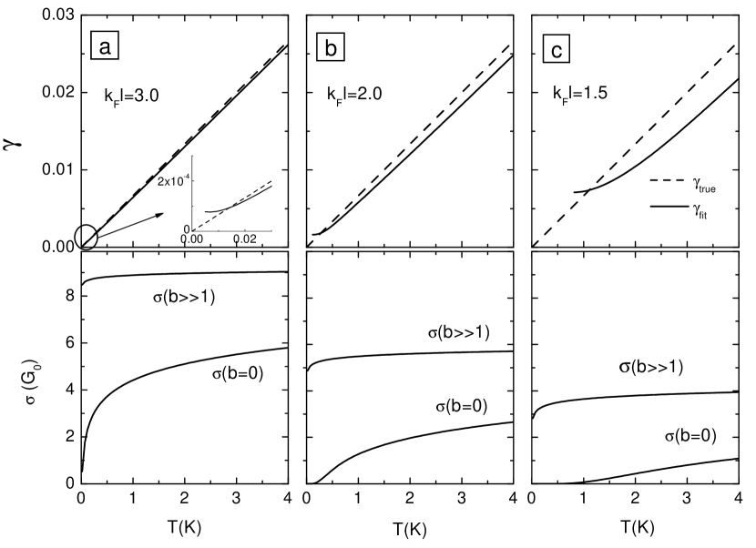
Figure 4: Illustration of low-temperature saturation of $\tau_{\varphi}$ obtained “experimentally” for the toy-model with different $k_{F}l$-values: (a) – $k_{F}l=3$ ($T_{1}=0.033$ K), (b) – $k_{F}l=2$, ($T_{1}=0.76$ K), and (c) – $k_{F}l=1.5$ ($T_{1}=3.7$ K). Upper panels show the temperature dependences of $\gamma_{\rm true}=T/T_{0}$, $T_{0}=150$ K (dashed lines) and $\gamma_{\rm fit}$ (solid lines) found from Eq. (48) with the use of $T$-dependence of $\sigma(b=0)$ and $\sigma(b\gg 1)$ shown in lower panels.

We conclude that the fitting of the MC with the use of the WLMC-expression cannot serve to obtain the real temperature behavior of the phase-breaking time at $\sigma(b=0)\lesssim G_{0}.$ Moreover, at such low conductivities the fitting procedure may yield seemingly a spurious saturation of the “experimentally extracted” dephasing rate at $T\to 0$.

IV.4 Effect of second-loop corrections to the MC: summary

We can summarize the results of the preceding sections as follows:

1. $B=0$; WL contribution. The terms of the second and third orders in $1/g$ cancel out in the relative interference correction in zero magnetic field. This means that for numerical reasons the temperature dependence of $\delta\sigma_{\rm WL}$ at $B=0$ is experimentally just the same as for the case $g\gg 1$, down to low enough values of $\sigma\simeq(2-3)G_{0}$:

   $${\delta\sigma_{\rm WL}(T)\over G_{0}}=-\beta\ln\left(\tau_{\varphi}(T)\over\tau\right),\mbox{ where }\beta=1.$$ (57)

2. $B\neq 0$; no interaction. The terms of the second order in $1/g$ do not influence the shape of the magnetic field dependence of the interference correction leading only to the decreasing of the prefactor. Therefore, the MC due to suppression of the WL is described by Eq. (10a)

   $${\Delta\sigma(b)\over G_{0}}=\alpha_{WL}\left\{\psi\left({1\over 2}+{\gamma\over b}\right)-\psi\left({1\over 2}+{1\over b}\right)-\ln\gamma\right\},$$ (58)

   with the prefactor $\alpha_{WL}$ decreasing as $\alpha_{WL}=1-G_{0}/\sigma$ with lowering $\sigma$ down to $\sigma\simeq(2-3)G_{0}$.

3. Coulomb interaction; $1/\tau_{\varphi}\ll\Omega_{B}\ll T$. The combined effect of the weak localization and Coulomb interaction leads to magnetic-field dependent corrections to the conductivity of the same order in $1/g$ as in previous case. At high temperatures, $T\gg\Omega_{B}$, the main effect is in the $B$-dependence of the dephasing time, which is reflected in the correction to the high-$B$ asymptotics of the digamma-function formula, Eqs. (10) – (14),

   $$\delta[\Delta\sigma(B)]\sim{\pi^{2}\over 2}\left[{1\over\Omega_{B}\tau_{\varphi}(B)}-{1\over\Omega_{B}\tau_{\varphi}(0)}\right]\simeq{\pi^{2}\over 2g}{T\over\Omega_{B}}\ln\left({T\over g\Omega_{B}}\right).$$ (59)

   Also, in this range of $B$, the Maki-Thompson correction to the MC dominates over the DoS-correction in the Cooper channel.

4. Coulomb interaction, stronger magnetic field, $T\ll\Omega_{B}\ll 1/\tau$. The combined effect of the weak localization and Coulomb interaction yields a logarithmic contribution to the MC, $\delta\sigma=(G_{0}/\sigma)\ln[1/(\Omega_{B}\tau)]$. Therefore, the total prefactor $\alpha$ in the MC is given by $\alpha_{2}=1-2G_{0}/\sigma$. This suggests that if the MC is fitted by Eq. (10), in the range of magnetic fields $T\ll\Omega_{B}\ll 1/\tau$, the decrease of the prefactor $\alpha$ is due to the second-loop corrections. Note, that taking into account the contribution of the triplet channel to $\delta\sigma_{\rm CWL}$ (neglected above) reduces the contribution of e-e interaction to the prefactor of the logarithmic conductivity correction, similarly to the case of the first-order Altshuler-Aronov correction gornyi-unpub . We also recall that the correction due to interaction in the Cooper channel is dominated by the DoS correction at such magnetic fields.

5. $B>B_{tr}$. In this range of magnetic fields the logarithmic corrections to the MC vanish. However, there are $B$-independent corrections $\propto(G_{0}/\sigma)\ln(T\tau)$ coming from the second-loop contributions, both from the non-interacting contribution (WL in the unitary ensemble) and from the cross-term (Coulomb plus WL). These corrections are important at low enough conductivities, when they can give an appreciable contribution to the prefactor of the $T$-dependence of the high-$B$ conductivity.

6. Dephasing time. The fitting of the MC by the WLMC-expression gives a correct value of the dephasing rate for $\sigma(B=0)\gtrsim 3G_{0}$. The $T$-dependence of $\tau_{\varphi}$ is given by a solution of the self-consistent equation (6) rather than by the first iteration of this equation for intermediate conductances. When applied in the WI regime, $\xi_{O}<L_{\varphi}<\xi_{U}$, the WLMC-expression yields the value of $\gamma_{\rm fit}$ which is not proportional to the true dephasing rate, but contains information about the localization length, $\xi_{O}.$

The above results are illustrated in Fig. 5. In the WL-regime, the magnetoconductivity as a function of $b$ behaves differently in the four regions of the magnetic field, ${\rm I:}\ b<b_{\varphi},\ {\rm II:}\ b_{\varphi}<b<b_{T},\ {\rm III:}\ b_{T}<b<1,$ and ${\rm IV:}\ b>1$. Here $b_{\varphi}=\tau/\tau_{\varphi}=\gamma$ is given by the dephasing rate and $b_{T}=T\tau$ is set by the temperature. In the region I, the MC is quadratic. In the region II, the deviation from the WLMC-formula Eq. (10) is determined by the impact of the magnetic field on the dephasing, and therefore other second-loop corrections are irrelevant. The region II, however, shrinks to zero with decreasing conductance, $\sigma\to G_{0}$. In the region III, the $B$-dependence of the dephasing is no longer crucial. The MC is given by Eq. (10) and the value of the prefactor $\alpha$ is determined by the second-loop contributions, Eq. (47). If the fitting procedure is carried out in the range of $B$ involving the fields such that $b\gg b_{T},$ it is this value of the prefactor which is expected to be found experimentally. In the WI-regime, the region II disappears, while the value of the magnetic field $b_{\xi}$, where the crossover between the parabolic (region I) and logarithmic (region III) MC occurs, is determined by the localization length $\xi_{O}$: $b_{\xi}\sim(l/\xi_{O})^{2}$. The MC in the region I ($b<b_{\xi}$) is beyond the scope of the present paper. On the other hand, the MC in the region III has the same origin as in the WL-regime and can be fitted by Eq. (10).

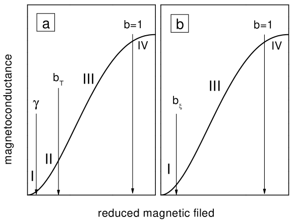
Figure 5: Schematic representation of the low-field quantum magnetoconductivity. Arrows show characteristic magnetic fields which mark off the regions with different behavior of magnetoconductivity (see text). It should be emphasized that the region III is much wider than regions I and II in our case (see Table 1).

In what follows we present the experimental results obtained in a wide range of conductivity. We start our analysis from the simpler case of high conductivity and follow what happens with the WL and MC with changing $T$ and $k_{F}l,$ and thus with the decreasing of the conductivity. We compare the experimental results with the above theory and find a quantitative agreement between the theory and the experiment.

V Experiment

In order to test quantitatively such refined theoretical predictions as presented above, suitable two-dimensional structures have to be used. First of all, the structures should be based on materials with single valley energy spectrum. Only one size-quantized subband should be occupied. Electrons should be only in the quantum well, no electrons should be in the doping layers. Finally, to avoid spin-dependent effects, the structures have to be symmetrical in shape in the growth direction. The single quantum well heterostructures based on $A_{3}B_{5}$ semiconductors met these requirements. We have investigated three types of the GaAs/In_xGa_1-xAs/GaAs single quantum well structures. They are distinguished by a “starting” nominal disorder that is achieved by a different manner of doping.

V.1 Experimental details and samples

The heterostructures with 80Å-In_0.2Ga_0.8As single quantum well in GaAs were grown by metal-organic vapor-phase epitaxy on a semi-insulator GaAs substrate. Structure H451 with high starting disorder had $Si-\delta-$doping layer in the center of the quantum well. The electron density $n$ and mobility $\mu$ in this structure were $n=0.89\times 10^{16}$ m^-2 and $\mu=0.23$  m²/Vs. Structure Z88 had lower starting disorder because the doping $\delta$ layers were disposed on each side of the quantum well and were separated from it by the 60 Å spacer of undoped GaAs. The parameters of structure Z88 were $n=5.1\times 10^{15}$ m^-2 and $\mu=1.3$  m²/Vs. Finally, the third structure 3509 had not $\delta$ doping layers. The conductivity of this structure was less than $10^{-2}\,G_{0}$ at liquid helium temperatures. The thickness of undoped GaAs cap layer was 3000 Å for all structures. The samples were mesa etched into standard Hall bars and then an Al gate electrode was deposited by thermal evaporation onto the cap layer of the structures H451 and Z88 through a mask. Varying the gate voltage $V_{g}$ from $0.0$ to $-3..-4$ V we decreased the electron density in the quantum well and changed $k_{F}l$ from $9-30$, for different samples, down to $\simeq 1$ (the values of $k_{F}l$ and $B_{tr}$ have been experimentally found as described in Appendix D). The conductivity of structure 3509 was changed via illumination by light of a incandescent lamp through a light guide. Due to persistent conductivity effect we were able to increase the conductivity and electron density for this structure up to approximately $60\,G_{0}$ and $5\times 10^{15}$ m^-2, respectively, changing the duration and intensity of illumination. Several samples of each structures have been measured and they all demonstrate the universal behavior.

V.2 Overview of the experimental results

The temperature dependences of the zero-$B$ resistivity $\rho$ measured at several $k_{F}l$-values controlled by the gate voltage for one of the samples made from structure Z88 are presented in Fig. 6(a). A thorough analysis of these dependences has been done in Ref. WLtoSL, . It has been shown that the $\sigma$-versus-$T$ dependences are close to the logarithmic ones for $k_{F}l\gtrsim 2$ over the actual temperature range. For the lower $k_{F}l$- values, when the conductivity is less than $e^{2}/h,$ a significant deviation from the logarithmic behavior is observed. The temperature dependences of conductivity are well described within the framework of the conventional theory of the quantum corrections down to $k_{F}l\simeq 2$. It has been also shown that the interference contribution to the conductivity for $B=0$ exceeds the contribution due to the electron-electron interaction in $3-5$ times.

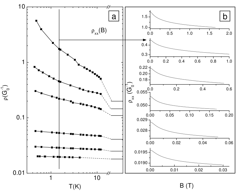
Figure 6: (a) The temperature dependence of the resistivity for structure Z88, measured at different $k_{F}l$ values: 1.6; 2.2; 2.9; 7.7; 12.8; 17.9 (from the top to the bottom). Horizontal lines show the values of $\sigma_{0}^{-1}=(\pi k_{F}lG_{0})^{-1}$ where $k_{F}l$ was found as described in Appendix D. (b) The $\rho_{xx}$-versus-$B$ dependences measured for $k_{F}l$ from the left panel at $T=1.5$ K.

The experimental magnetic-field dependences of $\rho_{xx}$ measured at $T=1.5$ K for the different $k_{F}l$-values are presented in Fig. 6(b). We restrict our consideration to the range of low magnetic field. In these fields the negative MR is completely determined by the interference effects which is subject of this paper. The high-magnetic-field MR and the role of electron-electron interaction have been studied in details in Ref. ourKee, and we will not consider them here. Even a cursory examination of Fig. 6(b) shows that the MR-curves are close in the shape for all $k_{F}l$-values, while the magnitude of the resistivity $\rho$ at low temperature is varied by more than two orders. This is more clearly seen from Fig. 7 where $\Delta\sigma(B)=1/\rho_{xx}(B)-1/\rho_{xx}(0)$ plotted as a function of reduced magnetic field, $b=B/B_{tr}$. Let us now analyze the experimental results starting with the case of high conductivity.

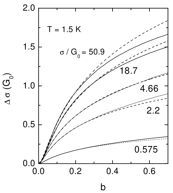
Figure 7: (a) The value of $\Delta\sigma$ as a function of reduced magnetic field, $b=B/B_{tr}$, measured for structure Z88 at $T=1.5$ K and different $k_{F}l$ values. Solid curves are the experimental data, dashed curves are the best fit by Eq. (10) with $\gamma$ and $\alpha$ given in Table 1.

V.2.1 High conductivities, $\sigma>20\,G_{0}$

In the case of sufficiently high zero-$B$ conductivities, $\sigma>20\,G_{0},$ the value of $k_{F}l>6$ is large enough and $\delta\sigma\ll\sigma_{0}$ in our temperature range. Therefore the use of WLMC-expression (10) is really warranted. For structure Z88, the results of the fit over the magnetic field range from 0 to 0.25 $B_{tr}$ with $\alpha$ and $\gamma=\tau/\tau_{\varphi}$ as fitting parameters are presented in Fig. 7 by dashed lines (the fit over narrower magnetic field range gives the close values of the fitting parameters to an accuracy of $15$%). The corresponding values of $\alpha$ and $\gamma$ are given in Table 1. It is evident that Eq. (10) well describes the experimental data. As seen from Fig. 8, where the results of such a data treatment are collected for all the structures, the prefactor $\alpha$ is close to unity that agrees with the low value of $\gamma<2\times 10^{-2}\ll 1$. Thus we conclude that the fitting procedure gives the value of $\tau_{\varphi}$ which can be directly attributed to the phase relaxation time.

Let us compare the extracted values of the dephasing time with the theory of the dephasing outlined in Section II.1. The experimental dependences of $\tau_{\varphi}(\sigma)$ are presented in Fig. 9. In the same figure we show the solution of Eq. (8) with $F_{0}^{\sigma}$ from the range $-0.45...-0.25$ that corresponds to $K_{ee}=0...0.55$ obtained for the structures presented here in Ref. ourKee, . As seen the experimental data are in satisfactory agreement with the theory of Ref. Aleiner379, . At first glance, it seems that we are able to determine the value of $F_{0}^{\sigma}$ from experimentally obtained values of the phase-breaking time. However, our analysis shows that the total uncertainty in determination of the phase relaxation time due to the neglect of the magnetic field dependence of the dephasing rate and due to the influence of ballistic effects our1 can be estimated as $20-30$% that obviously does not allow us to determine $F_{0}^{\sigma}$ by this way reliably. Thus, we assess the dephasing rate obtained experimentally for high conductivity as agreeing with the theoretical prediction.

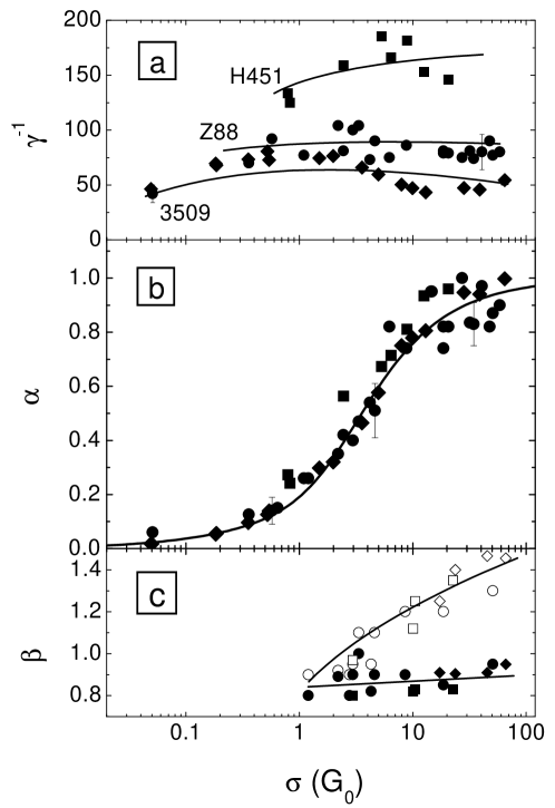
Figure 8: The conductivity dependence of the fitting parameters $\gamma^{-1}$ (a) and prefactor $\alpha$ (b) for structures Z88 (circles), H451 (squares), and 3509 (diamonds), $T=1.5$ K. (c) The experimental value of the prefactor $\beta$ in the temperature dependence of the interference quantum correction at $B=0$ (full symbols) and the slope of the experimental $\sigma$-versus-$\ln\,T$ dependence (open symbols) as functions of the conductivity at $T=1.5$ K for structure Z88. Curves in all panels are provided as a guide for the eye.

Table 1: The parameters for the structures Z88 ($T$-dependent quantities are given at T=1.5 K).

$\sigma(G_{0})$	$k_{F}l$	$B_{tr}({\rm Tesla})$	$\alpha$	$\tau_{\varphi}$ ($10^{-12}$ s)	$\gamma^{-1}$	$b_{T}$
50.9	17.9	0.029	0.9	23.3	69	0.073
18.7	7.7	0.12	0.79	13.6	73	0.037
4.66	2.9	0.64	0.53	9.1	96	0.019
2.2	2.2	1.06	0.35	7.8	104	0.015
0.575	1.6	1.64	0.14	5.9	92	0.013

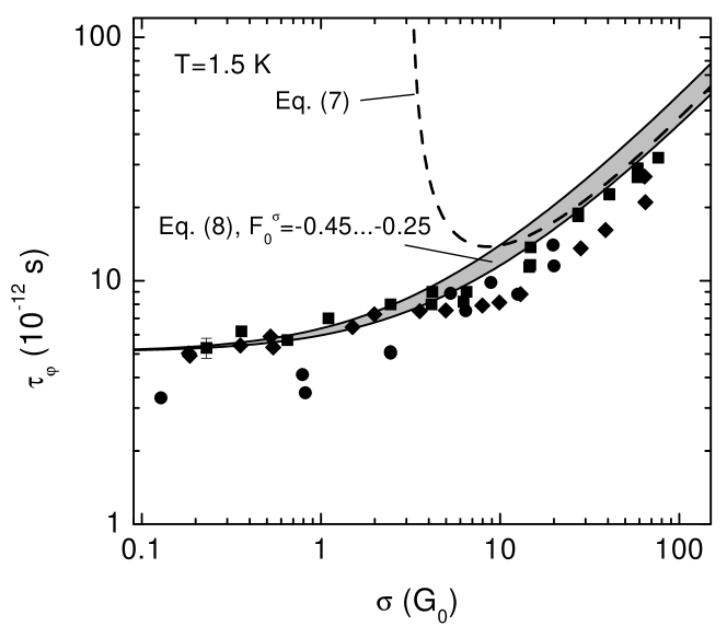
Figure 9: The conductivity dependence of $\tau_{\varphi}$ for $T=1.5$ K. Symbols are the experimental results [designations are the same as in Fig. 8(a)]. Dashed line is Eq. (7). Shadow strip represents the solutions of Eq. (8) found numerically for different values of $F_{0}^{\sigma}$ from the range $-0.25$ (upper bounding line) to $-0.45$ (lower one).

V.2.2 Intermediate and low conductivities, $\sigma<20\,G_{0}$

Although the WLMC-expression Eq. (10) describes the experimental results rather well (see Fig. 7), the correctness of the standard fitting procedure is questionable at these conductivity values. This is because the prefactor $\alpha$ reveals significant decreasing at $\sigma\lesssim 10\,G_{0}$ [see Fig. 8(b)], implying that the second fitting parameter $\gamma$ can in principle lose the meaning of the ratio of $\tau$ to $\tau_{\varphi}$. Therefore it is necessary either to understand the reasons of such a decrease or to use another theoretical model. In what follows we will try to employ the results of Section IV to describe the experimental data. We will show that the decrease of $\alpha$ can be understood within the framework of the weak localization theory extended to include the corrections of the second order in $1/g$. This means that the value of $\gamma_{\rm fit}$ extracted experimentally can be considered as the true value of $\tau/\tau_{\varphi}$ down to $\sigma\simeq 3G_{0}$. Remarkably, it turns out that even in the case of low zero-$B$ conductivities $0.1\,G_{0}<\sigma(B=0)<3\,G_{0},$ Eq. (10) describes the magnetoconductance shape perfectly (see Fig. 7). Moreover, surprisingly, this procedure gives the values of the parameter $\tau_{\varphi}$, which are close to that found from Eq. (8) down to $0.1\,G_{0}$ [see Fig. 9].

V.3 Comparison with the self-consistent theory of the MC

Before applying the approach developed in theoretical part of our paper to the experimental data, let us use the self-consistent Kleinert-Bryksin theory of the Anderson localization in a magnetic field. According to Ref. Bryksin, $\sigma(B)$ is the solution of the following self-consistent equation

$$\frac{\sigma}{G_{0}}=\frac{\sigma_{0}}{G_{0}}-\psi\left(\frac{1}{2}+\frac{l_{B}^{2}}{4l^{2}}+\frac{l_{B}^{2}}{4{\cal D}\tau_{\varphi}}\right)-\psi\left(\frac{1}{2}+\frac{l_{B}^{2}}{4{\cal D}\tau_{\varphi}}\right),$$ (60)

where ${\cal D}$ itself depends on $\sigma$ as ${\cal D}=\sigma/(e^{2}2\nu)$. The experimental $\sigma$-versus-$B$ dependences together with the solution of Eq. (60) for two values of the conductivity are shown in Fig. 10. It is evident that even for the relatively high conductivity $\sigma(B=0)=18.7\,G_{0}$ Eq. (60) describes the experiment noticeably worse than Eq. (10). In the case of low $\sigma$ the theory by Kleinert and Bryksin Bryksin gives fully incorrect behavior of $\sigma(B)$. One can try to improve the expression Eq. (60) treating self-consistently not only the diffusion constant but also the other $\sigma$-dependent quantities in Eq. (60), e.g. using the self-consistent equation (6) for $\tau_{\varphi}$. However, the numerical calculation shows that this modification of Eq. (60) does not change the results significantly.

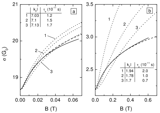
Figure 10: The conductivity as a function of magnetic field for structure Z88 for $\sigma(B=0)=18.7\,G_{0}$ (a) and $2.2\,G_{0}$ (b), $T=1.5$ K. Solid lines are the experimental results. Dotted lines are solutions of Eq. (60) with parameters shown in the tables, dashed lines are the best fit by Eq. (10) with parameters: $\alpha=0.8$, $\tau_{\varphi}=1.36\times 10^{-11}$ s, $B_{tr}=0.12$ T, $k_{F}l=7.7$ (a) and $\alpha=0.35$, $\tau_{\varphi}=0.76\times 10^{-11}$ s, $B_{tr}=0.95$ T, $k_{F}l=2.2$ (b).

VI Analysis of the experimental results: WL beyond one loop

VI.1 Prefactor in the WLMC-formula

Let us recall now the possible reasons which can in principle lead to decrease of the prefactor $\alpha$. They were considered in Section II.2. Below we will discuss some of them which could be relevant in our situation in more detail.

First of all, the decrease of $\alpha$ with decreasing $\sigma$ cannot obviously result from the violation of the diffusion regime, even for not very high $\sigma,$ because the ratio of $\tau_{\varphi}$ and $\tau$ is almost independent of the conductivity and remains high enough, as illustrated by Fig. 8 (a). Also, the range of magnetic fields, where the fitting of the MC-curves was performed, $b\lesssim 0.25$, does not include the ballistic range of fields, $B\gtrsim B_{tr}.$

Second, the decrease in the prefactor can in principle result from the contribution of the e-e interaction in the Cooper channel. It is apparent that treating the constant $\lambda_{0}$ in Eq. (18) as a fitting parameter, as is usually done, we are able to describe formally the experimental data by the sum of Eq. (15) and Eq. (10) with $\alpha=1$. What is the result? For example, processing the experimental $\Delta\sigma$-versus-$(B)$ curves for actual conductivity range ($\sigma$ at $T=1.5$ K is about $5\,G_{0}$) we have obtained that the value of seed constant $\lambda_{0}$ changes from $\lambda_{0}\simeq 4$ at $T=3$ K to $\lambda_{0}\simeq-0.62$ at $T=0.46$ K. Thus, the interaction constant changes with temperature not only the value but, moreover, the sign. It is clear that this result is meaningless. If we fix the interaction constant, say, at the value $\lambda_{0}=-0.62$ corresponding to the best fit for $T=0.46$ K, we obtain drastic positive magnetoresistance for $T=3$ K instead of negative one observed experimentally. Therefore, already the formal fitting procedure demonstrates that the electron-electron interaction in the Cooper channel is not responsible for the decrease of the prefactor with conductivity decrease under our experimental conditions.

However, as discussed in Section III, the actual value of the effective interaction constant $\lambda_{c}(T)$ yields a small corrections to the MC (as an example, see Fig. 3), which cannot be responsible for a drastic decrease of $\alpha$. This is mainly because the ratio $E_{F}/T\sim 10^{2}-10^{3}$ is very large in structures investigated. Therefore the relevance of the interaction corrections in the Cooper channel can be ruled out in the present experiment. Also, we see from Fig. 11 that temperature dependence of the prefactor is determined by the $T$-dependence of the conductivity rather than by the $T$-dependence of the effective interaction in the Cooper channel, $\lambda_{c}(T)$,

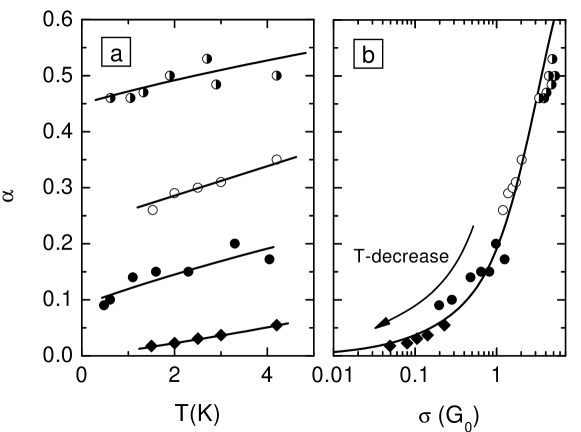
Figure 11: The prefactor $\alpha$ plotted against the temperature (a) and conductivity (b) when the latter changes with temperature. Circles correspond to structures Z88 when the value of $k_{F}l$, controlled by the gate voltage, is $1.6$ (solid circles), $2.0$ (open circles), and $2.9$ (half-filled circles); diamonds are data for structure 3509 with $k_{F}l\simeq 1.5$. Solid lines are provided as a guide for the eye, the line in (b) is just the same as in Fig. 8 (b).

Let us finally apply the approach described in Section IV. Recall that the lowering of the conductivity (i) should not change the $T$-dependence of the interference correction in zero magnetic field [see Eq. (57)] and (ii) should not influence the shape of the magnetic field dependence of $\sigma$ leading only to lowering of the prefactor in dependence $\Delta\sigma(B)$ as given by Eq. (47).

The second point is in a full agreement with our experimental results. The fitting of the MC was carried out in magnetic fields up to $b\gg b_{T}$ for all the curves, and therefore the prefactor in Eq. (10) is determined by the range $T\ll\Omega_{B},$ where it is given by Eq. (47). As seen from Fig. 7, Eq. (10) describes the data perfectly. The conductivity dependence of the fitting parameter $\alpha$ can be well described by Eq. (47), as Fig. 12 shows. We see that the second-order perturbative correction to the prefactor, arising in Eq. (46), describes the reduction of $\alpha$ down to $k_{F}l\sim 5$ corresponding to $\alpha\sim 0.8$ [Fig. 12 (a)]. Moreover, as discussed in Section IV.1 and in Appendix B, a better result can be achieved at lower conductivity if one replaces $\sigma_{0}$ by $\sigma(b\gtrsim 1)$ obtained for the unitary ensemble. This is illustrated by Fig. 12(b) in which an excellent agreement is evident down to $\sigma(b=1)\simeq(2-3)\,G_{0}$ corresponding to $\alpha\sim 0.2-0.3$. From a practical point of view, it is more convenient to use the zero-$B$ value of the conductivity in Eq. (47). We see from Fig. 12(c) that this also nicely describes the reduction of the prefactor $\alpha$, down to slightly higher values of $\alpha\sim 0.4-0.5$.

An important feature of the prefactor $\alpha$ is that it depends on the temperature mostly via the $T$-dependence of the conductivity, as follows from Fig. 11. Indeed, the values of the prefactor $\alpha(T)$ obtained for different temperatures perfectly lie on the same $\alpha$-versus-$\sigma(b=0)$ curve. We thus see that Eq. (47) proves to be rather universal. Both the temperature and the disorder strength affect the value of $\alpha$ only through their influence on the conductivity, so that the experimental points for different samples, densities, and temperatures are described by a single $\alpha$-versus-$\sigma$ curve in a broad range of conductivity.

It is tempting to interpret the above universality as an experimental confirmation of the scaling of the MC with the magnetic field. Then the conductivity dependence of the prefactor $\alpha$ might be interpreted as the experimentally determined $\beta$-function governing the renormalization of the MC. Although in Appendix B we have shown that there is no such scaling in the whole conductivity range (since it is violated in the third-loop order), an empirical formula resembling those used for the interpolation of the scaling $\beta$-function between the WL and SL regimes (see, e.g. Ref. AMP99, )

$$\alpha\simeq{\sigma\over 2}\ln\left({1+2/\sigma\over\sqrt{1+4/\sigma^{2}}}\right)$$ (61)

appears to describe the prefactor of the MC down to $\sigma(b=0)\simeq(1-2)\,G_{0}.$ This can be seen in Fig. 12(c), where Eq. (61) is presented by a dashed curve.

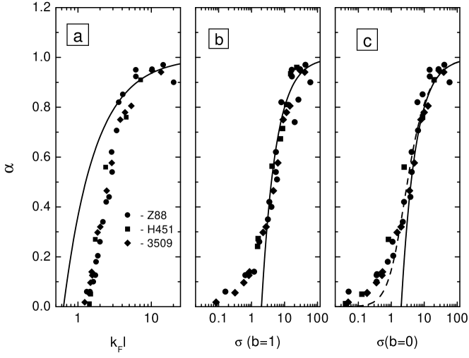
Figure 12: The value of prefactor $\alpha$ obtained for $T=1.5$ K as a function of $k_{F}l$ (a), $\sigma(b=1)$ (b), and $\sigma(b=0)$ (c). Solid lines are Eq. (47), dashed line is Eq. (61)

Another prediction of Section IV is that the temperature dependence of $\sigma$ at $B=0$ which includes both the weak localization and the electron-electron interaction correction for the intermediate conductances has to be the same as for the case $\sigma\gg G_{0}$,

$$\frac{\sigma(T)}{G_{0}}=\frac{\sigma_{0}}{G_{0}}-\beta\ln\left(\frac{\tau_{\varphi}(T)}{\tau}\right)+K_{ee}\ln\left(\frac{k_{B}T\tau}{\hbar}\right),$$ (62)

with $\beta=1$ (if one neglects the corrections in the Cooper channel). Our measurements show that in the heterostructures investigated, the temperature dependence of $\sigma$ is actually logarithmic within the temperature range from $0.45$ K to $4.2$ K while the value of $\sigma$ remains higher than $(1.0-1.5)\,G_{0}$, corresponding to $k_{F}l\gtrsim 2$. The slope of the $\sigma$-versus-$\ln{T}$ dependence as a function of $\sigma$ at $T=1.5$ K is shown in Fig. 8(c) by open symbols. In order to obtain the experimental value of the prefactor $\beta$ we have subtracted from these data the values of $K_{ee}$ which have been obtained just for the same samples in Ref. ourKee, . The final results are shown in Fig. 8(c) by solid symbols. Comparing figures 8(b) and 8(c) one can see that the prefactor $\alpha$ in MR noticeably deviates down from unity at $\sigma\simeq(7-8)\,G_{0}$, whereas the prefactor $\beta$ in the temperature dependence of $\sigma$ at $B=0$ remains close to unity down to $\sigma\simeq 1\,G_{0}$ (deviations from unity can be attributed to the contribution of the interaction in the Cooper channel). At lower $\sigma$ it is meaningless to determine $\beta$, because the temperature dependence of $\sigma$ no longer obeys the logarithmic law.

Figure 13, in which the $\sigma$-versus-$k_{F}l$ dependence is plotted, illustrates how strongly the quantum corrections can suppress the classical conductivity at low temperature. As seen the value of $\sigma$ is very close to the Drude conductivity at high $k_{F}l$ values and significantly less than that at low $k_{F}l$. For instance, the ratio $\sigma/\sigma_{0}$ for $T=1.5$ K is approximately equal to $0.4$ when $k_{F}l\simeq 2.5$, so that the interference and interaction corrections to the conductivity (from which the first one is the main WLtoSL ) strongly suppress the classical conductivity at low temperatures when the parameter $k_{F}l$ is small enough.

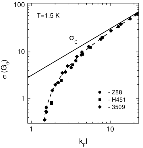
Figure 13: The conductivity at T=1.5 K as a function of $k_{F}l$. The value of $k_{F}l$ was obtained as described in Appendix D. Dashed line is provided as a guide for the eye, solid line is $\sigma_{0}=\pi k_{F}lG_{0}$

We arrive at the conclusion that using Eq. (10) we obtain reliably the value of the phase relaxation time with decreasing the conductivity down to the value of about $3\,G_{0}$. As seen from Fig. 9 the values of $\tau_{\varphi}$ found in this way demonstrate a good agreement with the dephasing theory.Aleiner379 Taking into account terms of the second order in $1/g$ in the WL theory allows us to understand quantitatively the magnetic field and temperature dependences of the conductivity for two-dimensional structures with different nominal disorder down to the value of the zero-$B$ conductivity about $\sim e^{2}/h$. The maximal value of the weak localization correction reaches $80-90$% of the Drude conductivity at lowest temperature, $T=0.45$ K. For the structures investigated this corresponds to the value of the parameter $k_{F}l$ close to two.

VI.2 Temperature dependence of the dephasing rate

In this subsection we consider the temperature dependence of $\tau_{\varphi}$ extracted from the fitting of the MC by the WLMC-expression Eq. (10). In accordance with the theory [see equations Eq. (6) and Eq. (8)] we plot the experimental values of $\tau_{\varphi}^{-1}$ as a function of $T$ in Fig. 14 (a). As seen from this figure, the temperature dependence of $\tau_{\varphi}$ can be perfectly described by the linear-in-$T$ function $\tau_{\varphi}^{-1}=T/T_{0}$ and, thus, $\tau_{\varphi}$ tends to infinity when $T$ goes to zero, when $k_{F}l\gtrsim 5$. At lower values of $k_{F}l,$ however, a linear extrapolation of $\tau_{\varphi}^{-1}$-versus-$T$ dependence gives a nonzero value of $\tau_{\varphi}$ at zero temperature. Such a behavior of $\tau_{\varphi}$ with temperature, known as phenomenon of low-temperature saturation of the phase relaxation time, was a central point of storm discussion in the literature during the last few years (for the recent review of the problem and for relevant references see Ref. vonDelft, ). However, we demonstrate below that the results presented here have nothing to do with the saturation of the true dephasing time $\tau_{\varphi}$ at $T\to 0.$

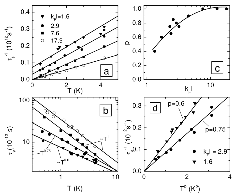
Figure 14: (a) The temperature dependence of $\tau_{\varphi}^{-1}$ for different values of $k_{F}l$, structure Z88. (b) The same experimental data as in (a), presented in double logarithmic scale. This plot illustrates that the $T$-dependence of $\tau_{\varphi}$ found from the fitting procedure can be satisfactorily described by the power law. (c) The value of exponent $p$ obtained from (b) as a function of $k_{F}l$ (symbols). Solid line is a guide for the eye. (d) The values $\tau_{\varphi}^{-1}$ plotted against $T^{p}$. Solid lines show extrapolation to $T=0$.

Let us first follow a standard route and plot our results in double-logarithmic scale. One can see that the experimental $T$-dependences of $\tau_{\varphi}$ (found from $\tau_{\varphi}=\tau/\gamma_{\rm fit}$) are well described by the power law $\tau_{\varphi}=(T/T_{0})^{-p}$ [Fig. 14 (b)]. The exponent $p$ is close to unity in wide $k_{F}l$-range from $20$ to $5,$ and slowly decreases when $k_{F}l$ becomes smaller [Fig. 14 (c)]. If we replot the experimental data in the $\tau_{\varphi}^{-1}$-vs-$T^{p}$ coordinates, we will see that $\tau_{\varphi}^{-1}$ again goes to zero when the temperature tends to zero [Fig. 14 (d)]. Thus, the analysis of the temperature dependence of the fitting parameter $\gamma_{\rm fit}$ shows that the seeming saturation in Fig. 14 can be in principle explained assuming that the dephasing rate is not linear-in-$T$ at low enough temperatures and conductances. Indeed, it looks plausible that the $1/T$-law changes to some $1/T^{p}$-law with $p<1$ when the parameter $k_{F}l$ decreases. Since $\tau_{\varphi}$ depends on the conductance $\sigma$ which itself depends on the temperature, the temperature dependence of $\tau_{\varphi}$ may be more complicated than simple $T^{-1}$ law.

Already the above consideration shows that our results cannot serve as the experimental confirmation of the low temperature saturation of the phase relaxation time. We emphasize, however, that as discussed above, the experimental value of $\tau_{\varphi}$ is merely the value of the fitting parameter of magnetoresistance. It can differ from the true phase relaxation time at $B=0$ when the conductance in not high, and this is precisely what happens in our experiment. In particular, this makes it of a little sense to analyze the behavior of exponent $p$. Moreover, as demonstrated in Section IV.3 and in Appendix C, the value of the fitting parameter $\gamma_{\rm fit}$ does saturate when the conductivity at $B=0$ becomes low. This implies that within the WI regime, the experimentally extracted value of the dephasing time deviates strongly from the true one. In fact, the two quantities are close only when $\sigma(b=0,T)\gtrsim 2G_{0}$, otherwise the fitting gives the information about the localization length instead of the true dephasing time. In Fig. 15 we compare the experimentally obtained values of $\gamma_{\rm fit}$ with those predicted by Eq. (48), using the experimental values of the conductivities and of the prefactor $\alpha$.

Unfortunately, it is not easy to determine experimentally the strong-$B$ value of the conductivity $\sigma(b\gg 1)$ involved in Eq. (48), because at strong magnetic fields the effects that are beyond the WL-theory become important. Therefore we have chosen to replace $\sigma(b\gg 1)$ by $\sigma(b=k_{F}l/2)$ to be confident that we are still dealing with the WL-conductivities. Hence we mistreat partially a $T$-independent ballistic contribution, so that the factor ${\cal C}$ in Eq. (48) cannot be determined reliably in this way. However, the temperature dependence of $\gamma_{\rm fit}$ should coincide with Eq. (48) up to a numerical factor. This is clearly seen in Fig. 15. Thus we confirm the validity of the expression Eq. (48) for the experimentally extracted value of the dephasing rate. As discussed in detail in Section IV.3, this expression yields a rather complicated $T$-dependence of $\gamma_{\rm fit}$ at low conductances, but this dependence cannot be directly connected with the $T$-dependence of the true $\tau_{\varphi}$.

To conclude this subsection, we have shown that the seeming low-$T$ saturation of the dephasing time at $k_{F}l\lesssim 5$ is nothing but an artifact of the fitting procedure, which fails to yield the true value of the dephasing rate at low conductances. At the same time, the shape of the MC is still perfectly described by the WLMC-expression at such conductances, but in effect with the localization length playing a role of the dephasing length.

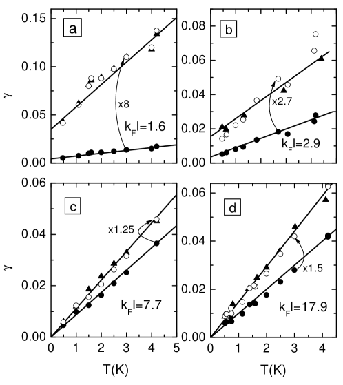
Figure 15: The temperature dependence of the parameter $\gamma$ found from the fit of the magnetoconductivity shape by Eq. (10) (circles), and $\gamma_{\rm fit}$ calculated from Eq. (48) with ${\cal C}=1/2$ (triangles) with the use of experimental values $\alpha$, $\sigma(b=0)$ and $\sigma(b=k_{F}l/2)$ [as $\sigma(b\gg 1)$] for $k_{F}l=1.6$ (a), $2.9$ (b), $7.7$ (c), and $17.9$ (d), structure Z88. Lines are provided as a guide for the eye.

VI.3 Discussion

Now we are in position to understand in what regime the 2D electron gas considered here is. This is determined by the characteristic length scales $\xi_{O}$, $\xi_{U}$ and $L_{\varphi}$ as was considered in the beginning of this paper (see Section I). As an example, Fig. 16(a) shows the relationship between these lengths for structure Z88 as a function of $k_{F}l$. The values of $\xi_{O}$ and $\xi_{U}$ have been calculated using Eq. (2) and Eq. (3), respectively, whereas the length $L_{\varphi}=\sqrt{D\tau_{\varphi}}$ has been found using $D$ and $\tau_{\varphi}$ obtained experimentally. It is clearly seen that the value of $L_{\varphi}$ is always less than both $\xi_{O}$ and $\xi_{U}$ when $k_{F}l\gtrsim 2$ and approaches $\xi_{O}$ with lowering $k_{F}l$. This is a direct manifestation of the fact discussed in Section IV.3: the experimentally extracted value of the phase-breaking length saturates with decreasing conductance at the value determined by the localization length $\xi_{O}$. This happens in a narrow range of $1.3<k_{F}l<2$, where the two curves in Fig. 16 come close to each other. Note, the low-temperature conductivity in this $k_{F}l$ range varies several-fold [see Fig. 16(b)] reaching values less than $G_{0}$. Analogous situation takes place for other heterostructures investigated.

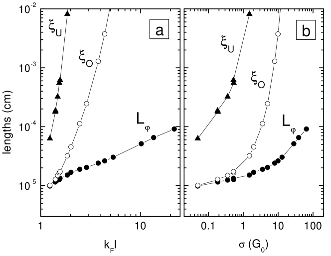
Figure 16: The lengths $L_{\varphi}$, $\xi_{O}$, and $\xi_{U}$ as a function of $k_{F}l$ (a) and $\sigma$ for $T=1.5$ K (b). The values of $\xi_{O}$ and $\xi_{U}$ have been calculated from Eq. (2) and Eq. (3), respectively, the length $L_{\varphi}$ is obtained using the quantity $D$ and $\tau_{\varphi}(T=1.5~{}\text{K})$ obtained experimentally. Structure Z88.

Thus, we infer that the electron gas in our case is in the WL regime at $T=1.5$ K for values of $k_{F}l$ larger than 2. For lower values of $k_{F}l$ the system is in the WI regime at $T=1.5$ K. We remind that the magnetoconductivity can still be described by the WLMC-expression Eq. (10) in the WI regime, even though the conductivity at low temperature becomes less than $G_{0}$ at low $k_{F}l$ values. This holds down to $k_{F}l\simeq 1$ which is the lowest value of $k_{F}l$ achieved in the present experiment and thus addressed in this paper. We therefore conclude that the theory of the magnetoresistance developed for the SL regime is inapplicable to our case.

VII Conclusion

We have studied the negative magnetoresistance of a two-dimensional electron gas in a weak transverse magnetic field $B$. The analysis has been carried out in a wide range of the zero-$B$ conductances, including the range of intermediate conductances (measured in units of $e^{2}/h$), $g\sim 1$. This range corresponds to the crossover between the low ($g\ll 1$) and high ($g\gg 1$) conductances. Furthermore, we have considered the regime of a “weak insulator”, when the zero-$B$ conductance is low $g(B=0)<1$ due to the localization at low temperature, whereas the Drude conductance is high, $g_{0}\gg 1,$ so that a sufficiently weak $B$ delocalizes electronic states.

The interpretation of experimental results obtained for 2D electron gas in GaAs/In_xGa_1-xAs/GaAs single quantum well structures has been based on the theory taking into account terms of high orders in $1/g$. We have shown that the standard weak localization theory is adequate for $\sigma\gtrsim 20G_{0}$. Calculating the corrections of the next order in $1/g$ to the MR, stemming from the interference contribution and from the mutual effect of WL and Coulomb interaction, we have expanded the range of the quantitative agreement between the theory and experiment down to significantly lower conductances $g\sim 1$.

We have demonstrated that at intermediate conductances the negative MR is described by the standard WLMC-expression (10), with a prefactor $\alpha$ which decreases with decreasing conductance. We have shown that at not very high $g$ the second-loop corrections dominate over the contribution of the interaction in the Cooper channel (the Maki-Thompson and DoS corrections). Thus the second-loop corrections appears to be the main source of the lowering of the prefactor, $\alpha=1-2G_{0}/\sigma$. This formula describes the experimentally obtained conductivity dependence of $\alpha$, provided that the fitting is performed in a broad range of magnetic fields, including those where $\Omega_{B}\gg T.$ The fitting of the MR allows us to measure the true value of the phase breaking time within a wide conductivity range, $\sigma=(3-60)G_{0}$. We have shown that the solution of the equation for $\tau_{\varphi}$ rather than its first iteration, describes well the $\tau_{\varphi}$-versus-$\sigma$ experimental dependence.

The quantitative agreement between the properly modified WL theory and experimental results obtained for intermediate conductances attests that the magnetoconductivity mechanism is unambiguously diffusive down to $\sigma\simeq 3\,G_{0}\simeq e^{2}/h$. Moreover, an agreement between the extended WL theory and experimental data persists down to significantly smaller zero-$B$ conductivity (WI-regime), provided that $k_{F}l>1$. In the WI regime, the MR can be still fitted by the WLMC-formula with a reduced prefactor, but the experimentally obtained value of the dephasing rate has nothing to do with the true one. The corresponding fitting parameter $\gamma_{\rm fit}$ is determined in the low-$T$ limit by the localization length and may therefore saturate with at $T\to 0$.

Finally, we have not investigated in detail the magnetoconductivity in the truly localized (at low-$T$) regime, when both the magnetic length and the phase-breaking length are greater than the localization length. The mechanism of a finite-$T$ conductivity in this situation is not completely clear, when the disorder is weak, $k_{F}l\gg 1$. The experiments on such insulators reveal features not captured by the conventional “textbook” hopping picture. A thorough study of the magnetoresistance in this regime is therefore of a great importance for understanding of the low-$T$ transport mechanism in such “weakly disordered” insulators.

Acknowledgment

We are grateful to I. L. Aleiner, A. D. Mirlin, D. G. Polyakov, P. Wölfle, and A. G. Yashenkin for interesting discussions and valuable comments. We thank O. I. Khrykin, V. I. Shashkin, and B. N. Zvonkov for growing the samples. This work was supported by the RFBR through Grants No. 02-02-17688, No. 03-02-16150, and No. 04-02-16626, the Program Russian Science School 2192.2003.2, the INTAS through Grant No. 1B290, the CRDF through Grants No. EK-005-X1 and No. Y1-P-05-11, the Russian Program Physics of Solid State Nanostructures, the Program of Russian Academy of Science, the Schwerpunktprogramm “Quanten-Hall-Systeme”, and the SFB195 der Deutschen Forschungsgemeinschaft.

Appendix A Maki-Thompson correction to the magnetoconductivity

In this Appendix we consider in detail the calculation of the Maki-Thompson correction. To analyze the MC arising due to the Maki-Thompson correction it is convenient to present this correction in the concise form,ayash ; ayash1 which is somewhat different from that used in Refs. Altshuler, ; AAKL-MIR, ; Larkin80, ,

$$\delta\sigma^{\rm MT} = \frac{4e^{2}}{\pi\hbar}\int\frac{d^{2}{\bf q}}{(2\pi)^{2}}\,\frac{D}{Dq^{2}+\Omega_{B}+1/\tau_{\varphi}}$$ (63)

$$\times \int_{-\infty}^{\infty}\,\frac{d\omega}{2T\sinh^{2}(\omega/2T)}\,\left[{\rm Im}\Pi_{c}({\bf q},\omega,\Omega_{B})\right]^{2}\,\left|\Lambda_{c}({\bf q},\omega,\Omega_{B})\right|^{2}.$$

The functions $\Pi_{c}$ and $\Lambda_{c}$ are given by Altshuler ; Larkin80

$$\Pi_{c}({\bf q},\omega,\Omega_{B}) = \ln\left(\frac{2E_{F}e^{\bf C}}{\pi T}\right)-\Psi_{c}({\bf q},\omega,\Omega_{B}),$$ (64)

$$\Psi_{c}({\bf q},\omega,\Omega_{B}) = \psi\left(\frac{1}{2}\left[1+\frac{Dq^{2}-i\omega+\Omega_{B}+\tau_{\varphi}^{-1}}{2\pi T}\right]\right)-\psi\left({1\over 2}\right),$$ (65)

$$\Lambda_{c}({\bf q},\omega,\Omega_{B}) = \left[\frac{1}{\lambda_{0}}+\Pi_{c}({\bf q},\omega,\Omega_{B})\right]^{-1}$$ (66)

$$= \left[\ln\left(\frac{T_{c}}{T}\right)-\Psi_{c}({\bf q},\omega,\Omega_{B})\right]^{-1}$$

where $\psi$ is digamma function. For simplicity, in Eq. (63) instead of the summation over quantized Cooperon momenta we integrate the Cooperon with the mass $\Omega_{B}$ over continuous $q$ (which is sufficient for $\Omega_{B}\gg\tau_{\varphi}^{-1}$).

Remarkably, the form Eq. (63) of the Maki-Thompson correction (in particular the frequency integral appearing there) is characteristic for the inelastic e-e scattering, see e.g. Ref. GornyiMirlin, ; ZNA, . The difference is that the polarization operator $\Pi_{c}$ and the effective interaction $\Lambda_{c}$ are taken in Eq. (63) in the Cooper channel, instead of the usual particle-hole channel, and the momentum integral involves a Cooperon. Similarly to conventional inelastic processes, the imaginary part of $\Pi_{c}$ comes only from the “dynamical” term $-i\omega$ in Eq. (65).

At $B=0$, the $q$-integral in Eq. (63) can be split into two parts, corresponding to small ($Dq^{2}\ll 2\pi T$) and large ($Dq^{2}\gg 2\pi T$) momenta. In the first contribution, one can neglect the terms $Dq^{2}$ and (for $g\gg 1$) $\tau_{\varphi}^{-1}$ in the function $\Psi_{c}$. Then the $q$-integral yields a logarithmic factor $\ln(T\tau_{\varphi})\sim\ln g$. Furthermore, one can replace $\Lambda_{c}$ by $\lambda_{c}(T)$. Performing then the frequency integral, we arrive at Eq. (16), in agreement with Ref. Larkin80, .

When calculating the contribution of large momenta, $Dq^{2}>2\pi T$, one can use the asymptotics of digamma function at large argument. Then the $q$-integral, having the structure $\int(dx/x)(T/x)^{2}\ln^{-2}(T_{c}/x)$ with $x=Dq^{2}$, is determined by the lower limit $x\sim 2\pi T$. The result of integration is also proportional to $\lambda^{2}_{c}(T)$, but in contrast to the contribution of small momenta, this integral does not produce a logarithmic term $\ln T\tau_{\varphi}.$ Therefore this contribution can be neglected at $g\gg 1$;Larkin80 however, with decreasing $g$ the two contributions become comparable.

In a finite magnetic field, the structure of Eqs. (63–66) suggests that the behavior of the Maki-Thompson correction depends on the value of the parameter $\Omega_{B}/2\pi T$. For $\Omega_{B}\ll 2\pi T$ the contribution of small $q$ yields the MR given by Eq. (20). The contribution of large $q$ to the MC depends only weakly on $B$ for any $g$, since to the leading order in $\Omega_{B}/2\pi T$ this contribution to $\delta\sigma^{\rm MT}$ is $B$-independent.

For $\Omega_{B}\gg 2\pi T$, one can again use the asymptotics of digamma function at large argument (now for the arbitrary momenta). The momentum integral is then determined by $Dq^{2}\sim\Omega_{B},$ yielding

$$\delta\sigma^{\rm MT}\propto\left(\frac{2\pi T}{\Omega_{B}}\right)^{2}\frac{1}{\ln^{2}(2\pi T_{c}/\Omega_{B})},\qquad\Omega_{B}\gg 2\pi T.$$ (67)

Therefore the Maki-Thompson contribution to the MC, $\Delta\sigma^{\rm MT}(B)=\delta\sigma^{\rm MT}(B)-\delta\sigma^{\rm MT}(0),$ saturates in the limit of high $B$ at $\Delta\sigma^{\rm MT}=-\delta\sigma^{\rm MT}(0),$ where $\delta\sigma^{\rm MT}(0)$ is given by Eq. (16). This makes it possible to describe the behavior of the Maki-Thompson correction to the MC by Eq. (10a) in the whole range of magnetic fields, with $\alpha_{\rm MT}=-\pi^{2}\lambda^{2}_{c}(T)/6$ and the replacement $1/\tau\to 2\pi T$,

$$\Delta\sigma^{\rm MT}(B)\simeq-{\pi^{2}\lambda^{2}_{c}(T)\over 6}{\cal H}(b/2\pi T\tau,1/2\pi T\tau_{\varphi}).$$ (68)

Although at $\Omega_{B}\gg T$ this expression gives the asymptotics different from Eq. (67), the precise way of the saturation of the Maki-Thompson contribution to the MC is irrelevant, since at $\Omega_{B}\gg T$ the DoS-term dominates $\Delta\sigma_{ee}^{\rm C}$ there, see Section IV.

Appendix B Scaling of the conductance in the cross-over between the unitary and orthogonal ensemble

One might be tempted to reformulate the results of Section IVA in terms of the renormalization group (RG) equation for the MC. That is, one might conjecture the existence of a single-parameter scaling of the MC with the magnetic field in the cross-over between the unitary and orthogonal ensembles. Indeed, the second-loop perturbative correction to the MC is logarithmic in $B$ which might correspond to the scaling of the MC with $l_{B}$, governed by the “cross-over” $\beta$-function,

$$\beta_{UO}=\beta_{O}-\beta_{U}=-{1\over{\mathsf{g}}}+{1\over 2{\mathsf{g}}^{2}},\qquad{\mathsf{g}}\gg 1.$$ (69)

In other words, given the value of the conductivity at $B=B_{tr}$ [Eq. (31)], one could be able to restore the MC for a fixed $T$ in the wide range of weaker magnetic fields ($l_{B}\ll L_{\varphi}$) including those where $\sigma(B,T)<G_{0}$, using a single RG-equation. Starting at $b\simeq 1$ from a high conductance, ${\tilde{\mathsf{g}}}_{0}(L_{\varphi})={\mathsf{g}}_{0}-(1/2{\mathsf{g}}_{0})\ln(L_{\varphi}/l)\gg 1,$ one would obtain the following expression for the renormalized conductance at weaker $B$,

$${\mathsf{g}}(l_{B},L_{\varphi}) \simeq {\tilde{\mathsf{g}}}_{0}(L_{\varphi})-\left(1-{1\over 2{\tilde{\mathsf{g}}}_{0}(L_{\varphi})}\right)\ln\left({l_{B}\over l}\right)$$ (70)

$$= {\mathsf{g}}_{0}-{1\over 2{\mathsf{g}}_{0}}\ln\left({L_{\varphi}\over l}\right)-\left(1-{1\over 2{\mathsf{g}}_{0}}\right)\ln\left({l_{B}\over l}\right)+{\cal O}(1/{\mathsf{g}}_{0}^{3}),$$ (71)

which agrees with the result of the perturbation theory.

However, an analysis of higher order corrections with the help of Eqs. 28 and 33 shows that there is no true scaling of the MC with $l_{B}.$ This can be seen in the third-loop order, implying that an “approximate scaling” with $l_{B}$ takes place only when the conductance is sufficiently high. On the other hand, the conventional scaling with the system size (in the present case – with the phase-breaking length $L_{\varphi}$) is applicable to the unitary-orthogonal cross-over.Lerner-Imry To illustrate this in the nontrivial case, when the localization length becomes $B$-dependent (see Section I), we fix the magnetic length to be the shortest macroscopic scale. We also set the value of the phase-relaxation length to lie between the two localization lengths,

$$l\ll l_{B}\ll\xi_{O}\ll L_{\varphi}\ll\xi_{U}.$$ (72)

In this situation, electrons are localized at $B=0$, but the magnetic field is chosen to delocalize the electronic states.

We start the scaling procedure at the microscopic scale, $L=l,$ where ${\mathsf{g}}\simeq{\mathsf{g}}_{0}\gg 1$ and increase $L$ up to $L=l_{B}$. The renormalization on such scales ($L<l_{B}$) is governed by the orthogonal $\beta$-function (33), and we get

$${\mathsf{g}}(L)={\mathsf{g}}_{0}-\ln\left({L\over l}\right)+{\cal O}\left({\ln(L/l)\over{\mathsf{g}}_{0}^{3}}\right).$$ (73)

At scales larger than $l_{B}$, the scaling is governed by the unitary $\beta$-function (28). The starting conductance is given by ${\mathsf{g}}(L=l_{B})={\mathsf{g}}_{0}-\ln(l_{B}/l)\gg 1$ and we find (for brevity, we measure the lengths in units of $l$ below),

$${\mathsf{g}}(L) = {\mathsf{g}}(l_{B})-{1\over 2{\mathsf{g}}(l_{B})}\ln\left({L\over l_{B}}\right)+{\cal O}(1/{\mathsf{g}}^{3})$$ (74)

$$\simeq {\mathsf{g}}_{0}-{1\over 2{\mathsf{g}}_{0}}\ln L-\left(1-{1\over 2{\mathsf{g}}_{0}}\right)\ln l_{B}-{1\over 2{\mathsf{g}}_{0}^{2}}\ln l_{B}\left[\ln L-\ln l_{B}\right].$$

The first three terms in this expression coincide with Eq. (71). The term containing the factor $1-1/2{\mathsf{g}}_{0}$ in Eq. (74) leads to the decrease of the prefactor $\alpha$ and has been already discussed above. One can see, however, that the last term $\sim{\cal O}(1/{\mathsf{g}}_{0}^{2})$ in Eq. (74) appears to violate the scaling of the MC with $l_{B},$ as seen from the comparison of Eq. (74) and Eq. 71: this term is absent in Eq. (71). Note that this term cannot be canceled out by higher terms in the expansion of $\beta$-functions because the $1/{\mathsf{g}}^{3}$-terms vanish in both Eq. (33) and Eq. (28). Taking a derivative of ${\mathsf{g}}(L,l_{B})$ with respect to $l_{B}$, one finds that it does not depend solely on the value of ${\mathsf{g}}(L,l_{B})$ itself. In particular, the term of the type ${\mathsf{g}}_{0}^{-2}\ln L$ arises, meaning the failure of the conjectured scaling equation Eq. (69) in the ${\cal O}(1/{\mathsf{g}}^{2})$ order.

The above standard scaling procedure allows one to estimate the localization length $\xi_{UO}$ at finite $B$ from the equation $g(\xi_{UO})\simeq 0$, yielding

$$\xi_{UO}(B)\sim l_{B}\exp\left([\pi k_{F}l/2-\ln(l_{B}/l)]^{2}\right),$$ (75)

in agreement with Ref. Lerner-Imry, .

Thus, while the scaling of the magnetoconductance with $B$ does not exist at low renormalized conductance, one can nevertheless use the formula Eq. (71) with ${\tilde{\mathsf{g}}}_{0}$ found at high fields $b\gtrsim 1$ in a rather wide range of fields. This implies that the effective prefactor $\alpha$ found from the fitting of the MC by the WL expression can be approximated by

$$\alpha_{WL}\simeq 1-{G_{0}\over\sigma(b\simeq 1,T)},$$ (76)

when the interaction corrections are neglected.

Appendix C Dephasing rate extracted from WLMC-formula

In this Appendix we derive a general expression for the experimentally extracted value of $\gamma_{\rm fit}$. We start with the reiteration of the scheme used for the derivation of the WLMC-expression and its generalization including the second-loop terms. For simplicity, we will not consider the contribution of $\delta\sigma_{2}^{\rm{I}\times{\rm WL}}$ in this Appendix and concentrate on the interference corrections. The MC $\Delta\sigma(b)$ is defined as

$$\Delta\sigma(b)=\sigma(b)-\sigma(0).$$ (77)

This definition is obviously more general than $\Delta\sigma(b)=\delta\sigma(b)-\delta\sigma(0),$ frequently used for $g\gg 1,$ i.e. when the conductivity corrections are small, compared to the Drude conductivity $\sigma_{0}$.

For $g\gg 1$ it is sufficient to take into account only the one-loop WL corrections to $\sigma_{0}$ (below we measure the conductivities in units of $G_{0}$),

$$\sigma(b) = \sigma_{0}+\delta\sigma(b)\simeq\sigma_{0}+\psi\left({1\over 2}+{\gamma\over b}\right)-\psi\left({1\over 2}+{1\over b}\right)+\delta\sigma_{\rm ball},\quad b\ll 1,$$ (78)

$$\sigma(0) = \sigma_{0}+\delta\sigma(0)=\sigma_{0}+\ln\gamma+\delta\sigma_{\rm ball}.$$ (79)

Here $\delta\sigma_{\rm ball}$ accounts for the non-logarithmic contributions of the ballistic interfering paths with lengths $L\lesssim l$ and the non-backscattering processes.dmit In zero $B$ (and actually for $b\ll 1$) this contribution for the case of white-noise disorder (short-range impurities) reads dmit

$$\delta\sigma_{\rm ball}(b=0)=\ln 2.$$ (80)

Using Eqs. (77), (78), and (79), we see that the terms $\sigma_{0}$ and $\delta\sigma_{\rm ball}$ from (78) and (79) cancel out in Eq. (77), so that the one-loop magnetoconductivity $\Delta\sigma_{1}(b)$ is determined solely by the logarithmic conductivity corrections,

$$\Delta\sigma_{(1)}(b)=\psi\left({1\over 2}+{\gamma_{b}\over b}\right)-\psi\left({1\over 2}+{1\over b}\right)-\ln\gamma,\quad b\ll 1$$ (81)

which is just the standard WLMC-expression with $\alpha=1$.

It is worth emphasizing that the value of $\gamma$ extracted from the experiment with the use of Eq. (81) is mostly determined by $\gamma$ from the last term ($\ln\gamma$) in Eq. (81), i.e. it comes from $\delta\sigma(b=0)$. This can be seen from the asymptotics Eq. (14) of the MC at strong $B$. In particular, when the MC is logarithmic, the value of $\gamma_{b}$ entering into the first digamma function (i.e. related to the dephasing in a finite $B$, hence the subscript $b$) appears only in the subleading term ${\cal O}(\gamma/b)$, see Ref. Aleiner379, . This difference is, however, unimportant for the one-loop correction to the MC, but it becomes essential with lowering $g$.

Now we rewrite Eq. (81) in a slightly different form

$$\Delta\sigma_{(1)}(b) = \delta\sigma(b)-[\sigma(0)-\sigma_{0}]$$ (82)

$$\simeq \psi\left({1\over 2}+{\gamma_{b}\over b}\right)-\psi\left({1\over 2}+{1\over b}\right)+\delta\sigma_{\rm ball}-[\sigma(0)-\sigma(b\gg 1)].$$

Here we have used that $\sigma(b\gg 1)\simeq\sigma_{0}$ within the one-loop approximation, since the ballistic contribution is also suppressed by a strong magnetic field, $\delta\sigma_{\rm ball}(b\gg 1)\to 0$. We thus see that instead of $\ln\gamma$ a structure, expressed in term of conductivities, $\sigma(0)-\sigma(b\gg 1)-\delta\sigma_{\rm ball},$ appears.

When the second-loop perturbative contribution is included, we have an analogous expression, see Section IV.1

$$\Delta\sigma_{(1+2)}(b) = \left(1-\frac{1}{\sigma_{0}}\right)\left\{\psi\left({1\over 2}+{\gamma_{b}\over b}\right)-\psi\left({1\over 2}+{1\over b}\right)\right\}+\delta\sigma_{\rm ball}$$ (83)

$$- [\sigma(0)-\sigma(b\gg 1)].$$

The zero-$B$ conductivity, Eq. (79), remains unchanged, while the conductivity at strong $B$ is now renormalized by the second-loop diffuson correction, Eq. (31), $\sigma(b\gg 1)\simeq\sigma_{0}+(1/\sigma_{0})\ln\gamma.$ Recalling that $\alpha_{\rm WL}=1-1/\sigma_{0},$ we get

$$\Delta\sigma_{(1+2)}(b) = \alpha_{\rm WL}\left\{\psi\left({1\over 2}+{\gamma_{b}\over b}\right)-\psi\left({1\over 2}+{1\over b}\right)\right.$$ (84)

$$+ \left.\frac{1}{\alpha_{\rm WL}}\Big{[}\sigma(b\gg 1)-\sigma(0)+\delta\sigma_{\rm ball}\Big{]}\right\},$$

implying that the role of $\ln\gamma$ in the generalized WLMC-expression is played by the combination in the last term in Eq. (84),

$$\ln\gamma_{\rm fit}\to-\frac{1}{\alpha_{\rm WL}}\Big{[}\sigma(b\gg 1)-\sigma(0)+\delta\sigma_{\rm ball}\Big{]}.$$ (85)

Thus the experimentally extracted value of the parameter $\gamma_{\rm fit}$ is given by

$$\gamma_{\rm fit}={\cal C}_{\rm ball}\exp\left\{{1\over\alpha_{\rm WL}}\Big{[}\sigma(0)-\sigma(b\gg 1)\Big{]}\right\},$$ (86)

where ${\cal C}_{\rm ball}$ is determined by the ballistic contribution $\delta\sigma_{\rm ball}$ which depends on the character of disorder. For point-like impurities, ${\cal C}_{\rm ball}\simeq 1/2$.

It turns out that under the condition $\sigma(b\gg 1)\gtrsim 3G_{0}$ (when the second-loop expression for $\sigma(b)$ is sufficient), this expression is valid for arbitrary $\sigma(b=0),$ including $\sigma(b=0)\ll G_{0}$, i.e. in the WI regime.

Appendix D Experimental determination of the Drude conductivity

In this Appendix we describe how the values of $B_{tr}$ and $k_{F}l,$ playing a pivotal role in the theory of weak localization, can be obtained experimentally. Since $B_{tr}$ is expressed as $B_{tr}=\hbar/(2el^{2})$ where $l$ is elastic mean free path, it can be found from the Drude conductivity $\sigma_{0}=\pi k_{F}l$ and electron concentration $n=k_{F}^{2}/(2\pi)$. The electron concentration can be obtained from the Hall effect. The question is: how can one obtain $\sigma_{0}$?

In the case of relatively high conductivity the experimental low-temperature value of $\sigma$ instead of $\sigma_{0}$ is often used. Let us estimate an error for the concrete case of $\sigma_{0}=20\,G_{0}$ and $\gamma=\tau/\tau_{\varphi}=0.01$. The use of $\sigma=\sigma_{0}+G_{0}\ln{\gamma}\simeq 15.4\,G_{0}$ (the interaction correction is neglected) instead of $\sigma_{0}=20\,G_{0}$ for determination of $B_{tr}$ leads to overestimation of $B_{tr}$ by a factor of about $1.4$. In its turn this results in an overestimation of $\tau_{\varphi}$ found experimentally by just the same factor. Another possibility is to measure the high-$T$ value of the conductivity, believing that the quantum corrections are destroyed by temperature. However, at high temperatures the electron-phonon scattering comes into play. Also, the ballistic contribution ZNA of the e-e interaction is $T$-dependent, thus making it difficult to determine the true value of $\sigma_{0}$.

In this paper the value of the Drude conductivity has been obtained by subtraction of the both interference and interaction corrections from the experimental value of the conductivity at $B=0$, using Eq. (62). The value of $K_{ee}$ was measured for the structure presented here in Ref. ourKee, . It has been found that the value of $K_{ee}$ is about $0.3-0.5$ at $k_{F}l\gtrsim 5$ and decreases with $k_{F}l$-decrease, almost vanishing at the lowest $k_{F}l\simeq 2$. The right-hand side of Eq. (62) itself depends on the value of $\tau/\tau_{\varphi}$, which can be found from the negative magnetoresistance. Therefore, treating the interference induced negative magnetoresistance we used the successive approximation method applying both equations Eq. (10) and (Eq. 62). For the first approximation we set $\sigma_{0}$ equal to $\sigma$, found $B_{tr}$ and, then, determined $\gamma$ from the fit of magnetoresistance by Eq. (10) using it and $\alpha$ as fitting parameters. After that we substituted $\gamma$ into Eq. (62) and found the corrected value of $\sigma_{0}$ and so on. An output of this procedure is the value of the prefactor $\alpha$, the ratio $\tau/\tau_{\varphi}=\gamma$ and the value of the Drude conductivity $\sigma_{0}$. It is sufficient to make from five to eight iterations to achieve an accuracy in the determination of $\sigma_{0}$ and $\gamma$ better than 10%. So complicated method is not significant for high conductivity ($\sigma\gtrsim 50G_{0}$) when the quantum corrections are relatively small. It should be noted that in the above procedure we do not take into account the non-backscattering contribution to the weak localization, which gives an additional temperature independent positive interference contribution equal to $G_{0}\ln\,2$.dmit In view of this and all other facts not pointed out here, we estimate an error in determination of $\sigma_{0}$ to be about $\pm 0.5\,G_{0}$.

References

- (1) Also at A.F. Ioffe Physico-Technical Institute, 194021 St. Petersburg, Russia.
- (2) B.L. Altshuler and A.G. Aronov, in Electron-Electron Interaction in Disordered Systems, edited by A.L. Efros and M. Pollak, (North Holland, Amsterdam, 1985).
- (3) B.L. Altshuler, A.G. Aronov, D.E. Khmelnitskii and A.I. Larkin in Quantum Theory of Solids, edited by I.M. Lifshits, (MIR Publishers, Moscow, 1982).
- (4) P.A. Lee and T.V. Ramakrishnan, Rev. Mod. Phys. 57, 287 (1985).
- (5) A.M. Finkelstein, Sov. Sci. Rev. A. Phys. 14, 1 (1990).
- (6) I.L. Aleiner, B.L. Altshuler, and M.E. Gershenzon, Waves Random Media 9, 201 (1999).
- (7) L.P. Gor’kov, A.I. Larkin, and D.E. Khmelnitskii, Pis’ma Zh. Eksp. Teor. Fiz. 30, 248 (1979) [JETP Lett. 30, 228 (1979)].
- (8) E. Abrahams, P.W. Anderson, D.C. Licciardello, and T.V. Ramakrishnan, Phys. Rev. Lett. 42, 673 (1979).
- (9) B.L. Altshuler, A.G. Aronov, and D.E. Khmelnitsky, J. Phys. C 15, 7367 (1982).
- (10) I.V. Lerner and Y. Imry, Europhys. Lett. 29, 49 (1995).
- (11) S. Hikami, Phys. Rev. B 24, 2671 (1981).
- (12) I.V. Gornyi and A.D. Mirlin, Phys. Rev. Lett 90, 076801 (2003); Phys. Rev. B 69, 045313 (2004).
- (13) S. Hikami, A. Larkin and Y. Nagaoka, Prog. Theor. Phys. 63, 707 (1980).
- (14) B.L. Altshuler, D. Khmelnitzkii, A.I. Larkin, and P.A. Lee, Phys. Rev. B 22, 5142 (1980).
- (15) Strictly speaking, in this regime the phase-breaking length loses its meaning, since for electrons localized at the largest spatial scale is given by . In this sense, it is meaningful to use the quantity instead of . Then one can formally define through using the relation valid for delocalized electrons. It is such phase-breaking length which we use when the SL and WI regimes are considered.
- (16) B.I. Shklovskii and A.L. Efros, Electronic Properties of Doped Semiconductors, (Springer, New York, 1984); A.L. Efros and B.I. Shklovskii, in Electron-Electron Interaction in Disordered Systems, edited by A.L. Efros and M. Pollak, (North Holland, Amsterdam, 1985).
- (17) V.L. Nguyen, B.Z. Spivak, and B.I. Shklovskii, Zh. Exp. Teor. Fiz. 89, 1770 (1985) [Sov. Phys. JETP 62, 1021 (1985)]; B.I. Shklovskii and B.Z. Spivak, in Hopping Transport in Solids, edited by M. Pollak and B.I. Shklovskii (Elsevier Science Publishers B.V., New York, 1991).
- (18) U. Sivan, O. Entin-Wohlman and Y. Imry, Phys. Rev. Lett 60, 1566 (1988).
- (19) O. Entin-Wohlman, Y. Imry, and U. Sivan, Phys. Rev. B 40, 8342 (1989).
- (20) Y. Zhang and M.P. Sarachik, Phys. Rev. B 43, 7212 (1991).
- (21) D.E. Khmelnitskii and A.I. Larkin, Solid State Commun. 39, 1069 (1981); B. Shapiro, Philos. Mag. B 50, 241 (1984).
- (22) M.E. Gershenson, Yu.B. Khavin, A.G. Mikhalchuk, H.M. Bozler, and A.L. Bogdanov, Phys. Rev. Lett. 79, 725 (1997).
- (23) D. Vollhardt and P. Wölfle, Phys. Rev. Lett. 45, 842 (1980); Phys. Rev. B 22, 4666 (1980).
- (24) D. Vollhardt and P. Wölfle, in Electronic Phase Transitions, edited by W. Hanke and Yu.V. Kopaev, (Elsevier Science Publishers B.V., 1992).
- (25) M.J. Uren, R.A. Davies, M. Kaveh, and M. Pepper, J. Phys. C 14, 5737 (1981).
- (26) R.A. Davies and M. Pepper, J. Phys. C 16, L353 (1983).
- (27) S.-Y. Hsu and J.M. Valles Jr., Phys. Rev. Lett. 74, 2331 (1995).
- (28) M.Y. Simmons, A.R. Hamilton, M. Pepper, E.H. Linfield, P.D. Rose, and D.A. Ritchie, Phys. Rev. Lett. 84, 2489 (2000).
- (29) Y.Y. Proskuryakov, A.K. Savchenko, S.S. Safonov, M. Pepper, M.Y. Simmons, and D.A. Ritchie, Phys. Rev. Lett. 86, 4895 (2001).
- (30) G. Brunthaler, A. Prinz, G. Bauer, and V.M. Pudalov, Phys. Rev. Lett. 87, 096802 (2001).
- (31) P.T. Coleridge, A.S. Sachrajda, and P. Zawadzki, Phys. Rev. B 65, 125328 (2002).
- (32) G.M. Minkov, O.E. Rut, A.V. Germanenko, A.A. Sherstobitov, B.N. Zvonkov, E.A. Uskova, and A.A. Birukov, Phys. Rev. B 65, 235322 (2002).
- (33) Yu.A. Pusep, H. Arakaki, and C.A. de Souza, Phys. Rev. B 68, 205321 (2003).
- (34) M. Rahimi, S. Anissimova, M.R. Sakr, S.V. Kravchenko, and T.M. Klapwijk, Phys. Rev. Lett. 91, 116402 (2003).
- (35) E. Abrahams, S.V. Kravchenko, and M.P. Sarachik, Rev. Mod. Phys. 73, 251 (2001).
- (36) B.L. Altshuler, D.L. Maslov, and V.M. Pudalov, Physica E 9 (2), 209 (2001).
- (37) G.M. Minkov, A.V. Germanenko, O.E. Rut, A.A. Sherstobitov, B.N. Zvonkov, E.A. Uskova, and A.A. Birukov, Phys. Rev. B 64, 193309 (2001).
- (38) V.V. Afonin, J. Bergli, Yu.M. Galperin, V.L. Gurevich, and V.I. Kozub, Phys. Rev. B 66, 165326 (2002) and references therein.
- (39) A.V. Germanenko, G.M. Minkov, and O.E. Rut, Phys. Rev. B 64, 165404 (2001).
- (40) G.M. Minkov, O.E. Rut, A.V. Germanenko, A.A. Sherstobitov, V.I. Shashkin, O.I. Khrykin, and V.M. Daniltsev, Phys. Rev. B 64, 235327 (2001).
- (41) M.G. Vavilov and L.I. Glazman, Phys. Rev. B 67, 115310 (2003) and references therein.
- (42) It is worth noting that at contributions to the MC, non-perturbative in , are still very small and can be neglected. We do not consider such terms in this paper.
- (43) I.L. Aleiner and Ya.M. Blanter, Phys. Rev. B 65 115317 (2002).
- (44) T. Ludwig and A.D. Mirlin, cond-mat/0312325.
- (45) D.G. Polyakov and K.V. Samokhin Phys. Rev. Lett. 80, 1509 (1998).
- (46) W. Eiler, J. of Low Temp. Physics 56 481, (1984).
- (47) B.N. Narozhny, G. Zala, and I.L. Aleiner, Phys. Rev. B 65, 180202 (2002).
- (48) A.M. Finkelstein, Zh. Eksp. Teor. Fiz. 84, 168 (1983) [Sov. Phys. JETP 57, 97 (1983)]; Z. Phys. B: Condens. Matter 56, 189 (1984).
- (49) G. Zala, B.N. Narozhny, and I.L. Aleiner, Phys. Rev. B 64, 214204 (2001).
- (50) L. Li, Y.Y. Proskuryakov, A.K. Savchenko, E.H. Linfield, and D.A. Ritchie, Phys. Rev. Lett. 90, 076802 (2003).
- (51) E.A. Galaktionov, A.K. Savchenko, S.S. Safonov, Y.Y. Proskuryakov, L. Li, M. Pepper, M.Y. Simmons, D.A. Ritchie, E.H. Linfield, and Z.D. Kvon, cond-mat/0402139.
- (52) G.M. Minkov, O.E. Rut, A.V. Germanenko, A.A. Sherstobitov, V.I. Shashkin, O.I. Khrykin, and B.N. Zvonkov, Phys. Rev. B 67, 205306 (2003).
- (53) A similar situation occurs for the interaction correction to the conductivity in the ballistic regime (), see Ref. ZNA, , where the correction to the conductivity is determined by the -dependent renormalization of the impurity scattering cross-section (and hence of the transport mean free time) by Friedel oscillations.
- (54) A.P. Dmitriev, V.Yu. Kachorovskii, and I.V. Gornyi, Phys. Rev. B 56, 9910 (1997).
- (55) A.G. Groshev, S.G. Novokshonov, Fiz. Tverd. Tela (St. Petersburg) 42, 1322 (2000) [Phys. Solid State 42, 1361 (2000)]; see also I.V. Gornyi, A.G. Groshev, and S.G. Novokshonov, Fiz. Tverd. Tela (St. Petersburg) 43, 766 (2001) [Phys. Solid State 43, 799 (2001)].
- (56) A. Kawabata, J. Phys. Soc. Japan, 53, 3540 (1984).
- (57) V.M. Gasparyan and A.Yu. Zyuzin, Fizika Tverdogo Tela (Leningrad) 27, 1662 (1985) [Sov. Phys. Solid State 27, 999 (1985)].
- (58) H.-P. Wittman and A. Schmid, J. Low. Temp. Phys. 69, 131 (1987).
- (59) M.I. Dyakonov, Solid State Commun. 92, 711 (1994).
- (60) A. Cassam-Chenai and B. Shapiro, J. Phys. I 4, 1527 (1994).
- (61) G.M. Minkov, A.V. Germanenko, V.A. Larionova, S.A. Negashev and I.V. Gornyi, Phys. Rev. B 61, 13164 (2000).
- (62) I.V. Gornyi, G.M. Minkov, O.E. Rut, A.V. Germanenko, and A.A. Sherstobitov, unpublished.
- (63) S.V. Iordanskii, Yu.B. Lyanda-Geller, and G.E. Pikus, JETP Lett. 60, 206 (1994); F.G. Pikus and G.E. Pikus, Phys. Rev. B 51, 16928 (1995); N.S. Averkiev, L.E. Golub, G.E. Pikus, JETP 86, 780 (1998).
- (64) A.G. Mal‘shukov, K.A. Chao, and M. Willander, Phys. Rev. Lett. 76, 3794 (1996).
- (65) W. Knap, C. Skierbiszewski, A. Zduniak, E. Litwin-Staszewska, D. Bertho, F. Kobbi, J.L. Robert, G.E. Pikus, F.G. Pikus, S.V. Iordanskii, V. Mosser, K. Zekentes, and Y.B. Lyanda-Geller, Phys. Rev. B 53, 3912 (1996).
- (66) A. Zduniak, M.I. Dyakonov, and W. Knap, Phys. Rev. B 56, 1996 (1997).
- (67) I.V. Gornyi, A.P. Dmitriev, and V.Yu. Kachorovskii, JETP Lett. 68, 338 (1998).
- (68) T. Hassenkam, S. Pedersen, K. Baklanov, A. Kristensen, C.B. Sorensen, P.E. Lindelof, F.G. Pikus, and G.E. Pikus, Phys. Rev. B 55, 9298 (1997); S. Pedersen, C.B. Sorensen, A. Kristensen, P.E. Lindelof, L.E. Golub, and N.S. Averkiev, Phys. Rev. B 60, 4880 (1999); L.E. Golub and S. Pedersen Phys. Rev. B 65, 245311 (2002).
- (69) S.A. Studenikin, P.T. Coleridge, N. Ahmed, P. Poole, and A. Sachrajda, Phys. Rev. B 68, 035317 (2003).
- (70) E.L. Altshuler, B.L. Altshuler, and A.G. Aronov, Solid State Commun. 54, 617 (1985).
- (71) A.I. Larkin, Pis’ma Zh. Eksp. Teor. Fiz. 31, 239 (1980) [Sov. JETP Letters 31, 219 (1980)].
- (72) K. Maki, Progr. Theor. Phys. 39, 897 (1968); R.S. Thompson, Phys. Rev. B 1, 327 (1970).
- (73) B.L. Altshuler, A.G. Aronov, A.I. Larkin and D. E. Khmelntitskii, JETP 82, 768 (1981).
- (74) B.L. Altshuler, A.A. Varlamov, and M.Yu. Reizer, Zh. Eksp. Teor. Fiz. 84, 2280 (1983) [Sov. Phys. JETP 57, 1329 (1983)].
- (75) Here we neglect the Aslamazov–Larkin conductivity correction in the Cooper channel. This correction is important in the vicinity of superconducting transition caused by the inter-electron attraction varlamov-larkin . However, in the case of the Coulomb repulsion, this correction is irrelevant, both for the conductivity at and for the MC Alt-Varlamov .
- (76) A.I. Larkin and A.A. Varlamov in Handbook on Superconductivity: Conventional and Unconventional Superconductors edited by K. Bennemann and J.B. Ketterson, (Springer, Berlin, 2002) and references therein.
- (77) In the limit the Maki-Thompson term usually also dominates over the DoS-term (both corrections give rise to a parabolic MC there). This holds as long as the condition being fulfilled in most relevant cases (since , while cannot be too low at experimentally accessible temperatures).
- (78) P. Kleinert and V.V. Bryksin Phys. Rev. B 55, 1469 (1997).
- (79) D. Yoshioka, H. Fukuyama, and Y. Ono, Surf. Sci. 113, 537 (1982); J. Phys. Soc. Jpn. 50, 2143 (1981); ibid, 3419 (1981).
- (80) C.S. Ting, Phys. Rev. B 26, 678 (1982).
- (81) K.B. Efetov, Supersymmetry in Disorder and Chaos, Cambridge University Press, (1997).
- (82) F. Wegner, Z. Phys. B 35, 207 (1979); Phys. Rep. 67, 15 (1980); Nucl. Phys. B 316, 663 (1989).
- (83) E. Brezin, S. Hikami, and J. Zinn-Justin, Nucl. Phys. B, 165, 528 (1980).
- (84) A.G. Groshev, S.G. Novokshonov, and I.V. Gornyi, unpublished.
- (85) I.V. Gornyi, unpublished.
- (86) In order to match the result obtained from the expansion of the digamma-function, with as defined in Eq. (42), one should use a slightly different definition of in Eq. (39). This is related to the fact that Eq. (39) was obtained by using the momentum integration of the Cooperon instead of the summation over Landau levels. This redefinition of does not affect, however, the logarithmic in -terms appearing due to the interplay between the WL and Coulomb interaction.
- (87) B.L. Altshuler, D.L. Maslov, and V.M. Pudalov, Phys. Stat. Sol. (b) 218, 193 (2000).
- (88) J. von Delft, J. Phys. Soc. Jpn. 72 Suppl. A, 24 (2003).
- (89) I.V. Gornyi, A.G. Yashenkin, and D.V. Khveshchenko, Phys. Rev. Lett. 83, 152 (1999).
- (90) I.V. Gornyi and A.G. Yashenkin, unpublished.