Cavity QED in superconducting circuits: susceptibility at elevated temperatures

Abstract

We study the properties of superconducting electrical circuits, realizing cavity QED. In particular we explore the limit of strong coupling, low dissipation, and elevated temperatures relevant for current and future experiments. We concentrate on the cavity susceptibility as it can be directly experimentally addressed, i.e., as the impedance or the reflection coefficient of the cavity. To this end we investigate the dissipative Jaynes-Cummings model in the strong coupling regime at high temperatures. The dynamics is investigated within the Bloch-Redfield formalism. At low temperatures, when only the few lowest levels are occupied the susceptibility can be presented as a sum of contributions from independent level-to-level transitions. This corresponds to the secular (random phase) approximation in the Bloch-Redfield formalism. At temperatures comparable to and higher than the oscillator frequency, many transitions become important and a multiple-peak structure appears. We show that in this regime the secular approximation breaks down, as soon as the peaks start to overlap. In other words, the susceptibility is no longer a sum of contributions from independent transitions. We treat the dynamics of the system numerically by exact diagonalization of the Hamiltonian of the qubit plus up to 200 states of the oscillator. We compare the results obtained with and without the secular approximation and find a qualitative discrepancy already at moderate temperatures.

I Introduction

There is, currently, a substantial activity in the research into the physics of Josephson qubits. In particular many groups Buisson et al. (2003); Blais et al. (2004); Il’ichev et al. (2003); Irish and Schwab (2003) became interested in studying the systems composed of Josephson qubits and harmonic oscillators, e.g., microwave cavities, mechanical resonators etc. Thus the field starts to resemble quantum optics where atoms in cavities have been investigated for many years. On one hand there are many results which can be simply “translated” from the “language” of quantum optics to the “language” of solid state physics. On the other hand there are specific properties of the solid state devices that might require further research.

In this paper we study the dynamics of a two-level system (qubit) and a cavity at resonance. In quantum optics this regime is the most studied and interesting one. The corresponding Jaynes-Cummings model (for a review see Ref. Shore and Knight, 1993) has been widely investigated in the literature. Experimentally, however, the strong coupling regime is difficult to achieve and it is also a challenge to keep the atom in the cavity for a long time. In optical cavities the strong coupling regime was achieved only a decade ago Thompson et al. (1992). Rydberg atoms in superconducting cavities Raimond et al. (2001) provide the strong coupling regime and one can even perform quantum gates during the time of flight of the atom through the cavity.

In solid state devices, e.g., a Josephson qubit resonantly coupled to a damped strip-line superconducting cavity Blais et al. (2004), the ”atom” is permanently placed in the cavity. This should simplify the time constraints. Also, the strong coupling limit seems to be possible. Thus these circuits constitute very promising setups for exploring the strong coupling limit of cavity QED. Compared to optical cavities, one of the differences is the finite temperature of solid state devices. Moreover, even if the nominal temperature of the refrigerator is much lower than the cavity’s energy splitting, the hot photons can arrive via the leads connecting to the controlling circuits. Thus the elevated temperature regime is of substantial interest. We are aware of only one article addressing the finite temperature case, namely Ref. Cirac et al., 1991. In this paper we expand the domain of parameters as compared with Ref. Cirac et al., 1991. Namely we consider the case when both the qubit’s and the cavity’s dissipative rates are much smaller than the cavity-qubit coupling (Rabi-frequency) and both the cavity and the qubit are coupled to the finite temperature baths. Moreover we focus on the correlation functions of the cavity, e.g., cavity susceptibility. In solid state systems this quantity is particularly convenient to measure as it is related to the impedance of the strip-line cavity. The temperature-dependence of this impedance constitutes a direct tool for probing the number of photons in the cavity.

At low temperatures the dynamics is very simple. Only a few states are occupied and the susceptibility may be presented as a sum of Lorentzians, corresponding to a few transitions allowed from these states. E.g., at zero temperature only two transitions are relevant and the resonant peak of the uncoupled cavity is Rabi split by the qubit to two peaks. At high temperatures the frequencies of different allowed transitions are densely packed near the oscillator’s frequency. This situation is called Liouvillian degeneracy as, formally, different modes of the Liouville evolution operator are almost degenerate Maassen van den Brink and Zagoskin (2002). We show that the secular approximation, widely used within the Bloch-Redfield formalism, fails due to the Liouvillian degeneracy. The insufficiency of the secular approximation was already noticed in, e.g., Ref. Lehmann et al., 2003. In this situation one has to take more elements of the Redfield tensor into account than required by the secular approximation. On the other hand the optical master equation takes all the necessary elements into account and thus produces correct results.

II Experimental motivation

We follow the recent proposal, presented in Ref. Blais et al., 2004, in which a superconducting charge qubit, coupled capacitatively to a cavity formed in a coplanar waveguide, is shown to be a favorable system for reaching the strong coupling regime of cavity QED. Typical parameters are cavity resonance/atom transition frequency of $\omega_{0}/2\pi=10$ GHz, a vacuum Rabi-frequency of $g/2\pi=100$ MHz, a cavity lifetime of $1/\kappa=160$ ns (quality factor $Q=\omega_{0}/\kappa=10^{4}$), and an atom lifetime $1/\gamma=2\mu$s. The system is measured by detecting absorption and phase shift of microwaves sent through the waveguide. In this paper we calculate the linear response absorption of the system. Motivated by the experimental parameters we focus on the regime of strong coupling $(\kappa,\gamma\ll g)$, and also assume that cavity dissipation dominates over atom dissipation $(\gamma<\kappa)$. We note that the photon temperature in the cavity may be much higher than the base temperature of the cryostat, due to coupling to room temperature sources through the waveguide. By measuring the absorption spectra one may determine the photon temperature of the cavity.

III The Jaynes-Cummings model

Assuming the qubit to be at the degeneracy point Vion et al. (2002); Blais et al. (2004), and for the moment neglecting dissipation, we arrive at the Jaynes-Cummings model, described by the following Hamiltonian

$$H_{JC}=-\frac{1}{2}\omega_{qb}\sigma_{z}+\omega_{osc}\,a^{\dagger}a+\frac{g}{2}\,\sigma_{x}\left(a+a^{\dagger}\right)\ ,$$ (1)

where $\sigma$ operates on atom/qubit while $a,a^{\dagger}$ are ladder operators of the cavity/oscillator. We consider the resonant regime when $\omega_{osc}=\omega_{qb}=\omega_{0}$. The system’s spectrum for $g\ll\omega_{0}$ is shown in Fig. 1.

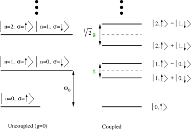
Figure 1: Spectrum of the Jaynes-Cummings model at resonance.

It is obtained by, first, analyzing the spectrum for $g=0$ (left side) and, then, lifting the degeneracies by the coupling $g$ (right side). Assuming $g\ll\omega_{0}$ we can take into account the coupling term only when it lifts the degeneracies in the spectrum. The ground state of the uncoupled system is $\left|g\right\rangle=\left|\uparrow,0\right\rangle$, which is non-degenerate. All other states are doubly degenerate, i.e. the states $\left|\uparrow,n\right\rangle$ and $\left|\downarrow,n-1\right\rangle$ form degenerate doublets for each $n\geq 1$. Every such doublet is split by the interaction. We can thus define the ”bonding” and the ”anti-bonding” states $|b/a,n\rangle\equiv 2^{-1/2}\left(\left|\uparrow,n\right\rangle\pm\left|\downarrow,n-1\right\rangle\right)$. The energies of these states are $E_{b/a,n}=n\omega_{0}\mp\sqrt{n}\,g/2$.

IV Oscillator/Cavity impedance

In ordinary cavity QED the atom susceptibility is usually probed. For the qubit-oscillator system the susceptibility of the oscillator (cavity) is the most easily measured quantity. It is defined as

$$\chi(t)=i\theta(t)\langle[q(t),q(0)]_{-}\rangle\ ,$$ (2)

where $q\equiv a^{{\dagger}}+a$. The Fourier transform is $\chi(\omega)=\chi^{\prime}(\omega)+i\chi^{\prime\prime}(\omega)=\int dt\chi(t)e^{i\omega t}$. The imaginary part of the susceptibility is proportional to the dissipative real part of the impedance, i.e., $\chi^{\prime\prime}(\omega)\propto{\rm Re}\,Z(\omega)$. For a closed system with quantum levels $\left|i\right\rangle$, with stationary occupation probabilities $\rho_{i}$, it can be presented as

$$\chi^{\prime\prime}(\omega) = \pi\sum_{i,f}\,\rho_{i}\,|\left\langle i\right|q\left|f\right\rangle|^{2}\,$$ (3)

$$\times \big{(}\delta(\omega-\omega_{fi})-\delta(\omega+\omega_{fi})\big{)}\ ,$$

where $\omega_{fi}\equiv(E_{f}-E_{i})/\hbar$. Thus it is a series of delta-peaks, corresponding to the allowed transitions.

At $T=0$ only the ground state is occupied and the two allowed transitions have frequencies $\omega_{g;\,b,1}=\omega_{0}-g/2$ and $\omega_{g;\,a,1}=\omega_{0}+g/2$ and the matrix elements $|\left\langle g\right|q\left|b,1\right\rangle|=|\left\langle g\right|q\left|a,1\right\rangle|=1/\sqrt{2}$. Thus the uncoupled oscillator’s peak at $\omega=\omega_{0}$ is split as shown in Fig. 2. This is called Rabi-splitting.

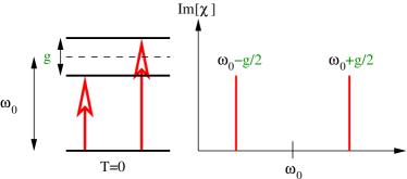
Figure 2: Transitions (left) resulting in a Rabi splitting of the cavity susceptibility (right), at $T=0$.

At $T>0$ higher energy states are occupied. The transitions are allowed only between neighboring doublets. There are two classes of allowed transitions. The ”bonding-bonding” or ”anti-bonding-anti-bonding” transitions correspond to the transition frequencies

$$\omega_{b,n-1;\,b,n}=\omega_{0}-{\frac{g}{2}}{\left(\sqrt{n}-\sqrt{n-1}\right)}\ ,$$ (4)

$$\omega_{a,n-1;\,a,n}=\omega_{0}+{\frac{g}{2}}{\left(\sqrt{n}-\sqrt{n-1}\right)}\ ,$$ (5)

with the matrix elements

$$|\left\langle b,n-1\right|q\left|b,n\right\rangle|=|\left\langle a,n-1\right|q\left|a,n\right\rangle|=$$

$$=\frac{1}{2}\left(\sqrt{n}+\sqrt{n-1}\right)\ .$$ (6)

They form the first class of transitions which all are positioned inside of the zero temperature Rabi-splitting. Analogously, the ”bonding-anti-bonding” transitions with frequencies

$$\omega_{b,n-1;\,a,n}=\omega_{0}+{\frac{g}{2}}{\left(\sqrt{n}+\sqrt{n-1}\right)}\ ,$$ (7)

$$\omega_{a,n-1;\,b,n}=\omega_{0}-{\frac{g}{2}}{\left(\sqrt{n}+\sqrt{n-1}\right)}\ ,$$ (8)

and matrix elements

$$|\left\langle b,n-1\right|q\left|a,n\right\rangle|=|\left\langle a,n-1\right|q\left|b,n\right\rangle|=$$

$$=\frac{1}{2}\left(\sqrt{n}-\sqrt{n-1}\right)$$ (9)

are all positioned outside the Rabi-splitting. Both classes of transitions are shown in Fig. 3.

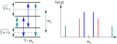
Figure 3: Transitions (left) and cavity susceptibility (right) at $T>0$. The central (blue) arrows correspond to ”bonding-bonding” and ”anti-bonding-anti-bonding” transitions, giving rise to the central two peaks in the spectrum. The outer (blue-green) arrows correspond to ”bonding-anti-bonding” transitions, giving the outer two peaks in the spectrum.

V Cavity dissipation

Due to the dissipation the delta functions should be widened to Lorentzians. At zero temperature the widths of the peaks are estimated as $\delta\omega=\omega_{0}/(2Q)$ (the factor $2$ is due to the reduced matrix element for each transition as compared to the original oscillator’s transition).

The problem is getting the line-shape at finite (relatively high) temperatures and high values of $Q$. Indeed, when temperature becomes of order $\omega_{0}$ more transitions become available. To estimate the heights of the peaks we note that the occupation probabilities of the doublets are estimated as $\rho_{n}\approx Z\exp(-n\omega_{0}/T)$. The matrix elements for the ”bonding-bonding” or ”anti-bonding-anti-bonding” transitions grow as $\propto\sqrt{n}$, while those for ”bonding-anti-bonding” transitions decay as $\propto 1/\sqrt{n}$. Thus we obtain a ”Poisson” distribution for the ”bonding-bonding” or ”anti-bonding-anti-bonding” peaks’ heights with the maximum at $n\approx T/\omega_{0}$. The heights of the ”bonding-anti-bonding” peaks decay with $n$. Therefore the highest peaks are situated at $\omega\approx\omega_{0}\pm\sqrt{\omega_{0}/T}\,g/4$.

The spacing between the dominant peaks ($\sim\frac{g}{2}\,\sqrt{\frac{\omega_{0}}{T}}$) thus decrease with temperature, while their width ($\sim\frac{2T^{2}}{Q\omega_{0}}$) increase with temperature. Around the cross-over temperature $T_{c}=\omega_{0}(gQ/4\omega_{0})^{2/5}$ the peaks start to overlap.

Thus, as the temperature grows, we have a transition from a quite ”un-harmonic” spectrum without Liouvillian symmetry, where all transition frequencies are different, to a spectrum which resembles that of two uncoupled linear oscillators, see Fig. 4. The widths of the peaks in these two cases behave qualitatively different. In the first (un-harmonic) case the widths grow with temperature, while in the second (harmonic oscillator) case they do not.

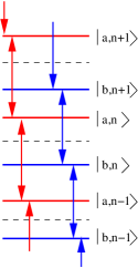
Figure 4: At high temperatures $T\gg\omega_{0}$ the “bonding” (blue) and “anti-bonding” (red) states form two almost equidistant spectrums. The non-harmonicity decreases as $\sqrt{n+1}-\sqrt{n}\approx 1/2\sqrt{n}$ for large $n$.

VI Qubit/atom dissipation

The qubit/atom is also subjected to dissipation, which will add to the peak widths in the susceptibility. At the degeneracy point of the qubit the longitudinal noise (coupled to $\sigma_{z}$) is suppressed to first order Vion et al. (2002). The transverse noise (coupled to $\sigma_{x}$) will induce transitions in the qubit, characterized by the rate $1/\gamma$. In terms of the Jaynes-Cummings eigenstates the qubit dissipation cause similar transitions as the cavity dissipation. A major difference is that the matrix elements for these transitions are independent of the oscillator state $n$. Thus, as long as the two sources of dissipation are of the same order of magnitude, the high temperature susceptibility will be determined by the cavity dissipation.

VII Bloch-Redfield formalism

We model the cavity/atom dissipation by coupling an observable $X/Y$ of a thermal bath to the $q/\sigma_{x}$-coordinate of the cavity/atom:

$$H=H_{JC}+qX+\sigma_{x}Y+H^{X}_{\rm bath}+H^{Y}_{\rm bath}\ .$$ (10)

One popular choice of a bath is the harmonic oscillator one Feynman and Vernon (1963); Caldeira and Leggett (1981). In this case $H_{\rm bath}=\sum_{i}\omega_{i}b^{\dagger}_{i}b_{i}$ and $X=\sum_{i}\lambda_{i}(b_{i}+b^{\dagger}_{i})$. However, as we are assuming weak dissipation and doing the lowest order calculation, the precise nature of the bath is unimportant and only the bath correlator $\langle X(t)X(0)\rangle$ matters.

The Bloch-Redfield equation Bloch (1957); Redfield (1957) is a kinetic equation for the reduced (qubit+cavity) density matrix:

$$\dot{\rho}_{mn}(t)+i\omega_{mn}\rho_{mn}(t)=\sum_{m^{\prime},n^{\prime}}R_{mnm^{\prime}n^{\prime}}\ \rho_{m^{\prime}n^{\prime}}(t)\ ,$$ (11)

where the Bloch-Redfield tensor is given by

$$R_{mnm^{\prime}n^{\prime}} = \lambda_{m^{\prime}mnn^{\prime}}+\lambda^{*}_{n^{\prime}nmm^{\prime}}$$ (12)

$$- \sum_{k}\delta_{mm^{\prime}}\lambda_{nkkn^{\prime}}+\delta_{nn^{\prime}}\lambda^{*}_{mkkm^{\prime}}\ ,$$

and

$$\lambda_{m^{\prime}mnn^{\prime}} = \left\langle m^{\prime}\right|q\left|m\right\rangle\left\langle n\right|q\left|n^{\prime}\right\rangle L_{X}(\omega_{nn^{\prime}})$$ (13)

$$+ \left\langle m^{\prime}\right|\sigma_{x}\left|m\right\rangle\left\langle n\right|\sigma_{x}\left|n^{\prime}\right\rangle L_{Y}(\omega_{nn^{\prime}})\ ,$$

where $L_{X}(\omega)$ is the Laplace transform of the cavity bath correlator

$$L_{X}(\omega)=\int_{0}^{\infty}dte^{-i\omega t}\langle X(t)X(0)\rangle\ .$$ (14)

Introducing the Fourier image of the unsymmetrized correlator $\langle X^{2}_{\nu}\rangle\equiv\int dt\langle X(t)X\rangle\,e^{i\nu t}$, we obtain

$$L_{X}(\omega)=-i\int\frac{d\nu}{2\pi}\,\frac{\langle X^{2}_{\nu}\rangle}{\nu+\omega-i0}\ .$$ (15)

Thus for the real part of $L_{X}$ which determines the transition rates we obtain ${\rm Re}\,L_{X}(\omega)=(1/2)\,\langle X^{2}_{\nu=-\omega}\rangle$. The imaginary part of $L_{X}$ is responsible for the energy shifts (Lamb shift). $L_{Y}(\omega)$ of the qubit bath is defined and treated analogously.

Considering a high quality cavity ($Q\gg 1$), and low qubit dissipation ($\gamma\ll\omega_{0}$), we limit ourselves to single photon exchange with the baths. The possible transition energies in Eq. (13) are $\omega_{nn^{\prime}}=\pm\omega_{0}+O(g)$, (see Eqs. (4)-(IV)). Furthermore we assume that the baths have no structure on the scale of the qubit-oscillator coupling $g$, leaving only one relevant parameter for relaxation $\langle X^{2}_{\omega_{0}}\rangle=\kappa/(1-e^{-\omega_{0}/T_{\kappa}})$, $\langle Y^{2}_{\omega_{0}}\rangle=\gamma/(1-e^{-\omega_{0}/T_{\gamma}})$, and one for excitation $\langle X^{2}_{-\omega_{0}}\rangle=e^{-\omega_{0}/T_{\kappa}}\langle X^{2}_{\omega_{0}}\rangle$, $\langle Y^{2}_{-\omega_{0}}\rangle=e^{-\omega_{0}/T_{\gamma}}\langle Y^{2}_{\omega_{0}}\rangle$, for each bath.

VII.1 The secular approximation

Looking for the slow dynamics of our system, on the time-scale given by the dissipation ($1/\kappa,1/\gamma$), we rewrite eq. (11) in the rotating frame

$$\dot{\tilde{\rho}}_{mn}(t)=\sum_{m^{\prime},n^{\prime}}R_{mnm^{\prime}n^{\prime}}\ \tilde{\rho}_{m^{\prime}n^{\prime}}(t)e^{i(\omega_{mn}-\omega_{m^{\prime}n^{\prime}})t}\ ,$$ (16)

where $\tilde{\rho}_{mn}(t)=\rho_{mn}(t)e^{i\omega_{mn}t}$ evolves slowly in time.

When there are no Liouvillian degeneracies the phase $(\omega_{mn}-\omega_{m^{\prime}n^{\prime}})t$ in the above expression rotates with a frequency of the order of $\omega_{0}\gg\kappa,\gamma$, except when $m=m^{\prime}$ and $n=n^{\prime}$, or $m=m^{\prime}$ and $n=n^{\prime}$. The secular approximation is a random-phase type of approximation, keeping only the corresponding elements of Redfield tensor, $R_{mnmn}$ and $R_{mmnn}$.

Within the secular approximation the Bloch-Redfield equation separates into a master equation governing the occupation numbers: $\dot{\rho_{nn}}(t)=R_{nnmm}\rho_{mm}(t)$, and a simple exponential decay of all off-diagonal elements of the density matrix: $\rho_{mn}(t)=\rho_{mn}(0)e^{(-i\omega_{mn}+R_{mnmn})t}$. In the susceptibility we find that the weights of the peaks are given by the steady-state occupation numbers, determined by the transition rates ($R_{nnmm}$), while the peak widths are given by the dephasing rates ($R_{mnmn}$).

VII.2 Liouvillian degeneracy

When difference between two transition frequencies $\omega_{mn}-\omega_{m^{\prime},n^{\prime}}$ ($m\neq m^{\prime}$ and $n\neq n^{\prime}$) becomes smaller than the transitions’ widths $\propto(\kappa,\gamma)$ the peaks start to overlap. In this case there is no justification for the secular approximation, and more elements of the Redfield tensor must be retained.

In the lowest order (single-photon transitions) the allowed transition (photon) frequencies are $\pm\omega_{0}+O(g)$, giving two possible values for $|\omega_{mn}-\omega_{m^{\prime}n^{\prime}}|=\{0,2\omega_{0}\}+O(g)$. Looking for slow dynamics we neglect the elements $R_{mnm^{\prime}n^{\prime}}$ corresponding to the Liouvillian modes with $|\omega_{mn}-\omega_{m^{\prime}n^{\prime}}|=2\omega_{0}+O(g)$. This is equivalent to a rotating-wave-approximation in the coupling to the bath. We keep, however, the elements $R_{mnm^{\prime}n^{\prime}}$ corresponding to the Liouvillian modes with $|\omega_{mn}-\omega_{m^{\prime}n^{\prime}}|=O(g)$. That is, grouping the elements of the density matrix $\rho_{mn}$ according to the energy difference $E_{m}-E_{n}=M\omega_{0}+O(g)$, we now couple only the elements with similar $M$, but leave the elements with different $M$ uncoupled. We also note that the Bloch-Redfield equation with this choise of the elements $R_{mnm^{\prime}n^{\prime}}$ is equivalent to the ”Quantum Optics” master equation:

$$\dot{\rho} = -i[H_{JC},\rho]+\kappa N_{\kappa}(2a^{\dagger}\rho a-aa^{\dagger}\rho-\rho aa^{\dagger})$$ (17)

$$+ \kappa(N_{\kappa}+1)(2a\rho a^{\dagger}-a^{\dagger}a\rho-\rho a^{\dagger}a)$$

$$+ \gamma N_{\gamma}(2\sigma^{+}\rho\sigma^{-}-\sigma^{-}\sigma^{+}\rho-\rho\sigma^{-}\sigma^{+})$$

$$+ \kappa(N_{\gamma}+1)(2\sigma^{-}\rho\sigma^{+}-\sigma^{+}\sigma^{-}\rho-\rho\sigma^{+}\sigma^{-})$$

where $N_{\kappa/\gamma}=1/(e^{\omega_{0}/T_{\kappa/\gamma}}-1)$ are the average occupation numbers of each bath at frequency $\omega_{0}$.

VIII Numerical approach

In our numerical studies we take into account the lowest $N$ states of the harmonic oscillator, and then check for convergence by increasing $N$. We work in the eigenbasis of the Jaynes-Cummings Hamiltonian (Eq. 1), which we obtain by numerical diagonalization.

We then rewrite the Bloch-Redfield equation (Eq. (11)) in a matrix form, i.e.

$$\dot{\rho}_{[mn]}(t)+i\omega_{[mn][mn]}\rho_{[mn]}(t)=\sum_{[m^{\prime}n^{\prime}]}R_{[mn][m^{\prime}n^{\prime}]}\ \rho_{[m^{\prime}n^{\prime}]}(t)\ ,$$ (18)

where $\hat{\rho}(t)=\rho_{[mn]}(t)$ now is a column vector of length $(2N)^{2}$ and $\hat{R}=R_{[mn][m^{\prime}n^{\prime}]}$ is a matrix of size $(2N)^{2}\times(2N)^{2}$, and $\hat{\omega}=\omega_{[mn][mn]}$ is a diagonal matrix of the same size. The solution can then be written

$$\hat{\rho(t)}=e^{(-i\hat{\omega}+\hat{R})t}\cdot\hat{\rho}(0),$$ (19)

which we evaluate by exact diagonalization of $-i\hat{\omega}+\hat{R}$, which is the bottleneck of the calculation since the size of this matrix grows with $N^{4}$.

Fortunately the property of the Redfield tensor to couple only elements of the density matrix $\rho_{mn}$ with similar energy difference $E_{m}-E_{n}\approx M\omega_{0}$, makes the matrix $\hat{R}$ block-diagonal. The size of each block is only $~{}4N\times 4N$, which makes the problem tractable up to hundreds of states in the cavity.

VIII.1 Cavity susceptibility

The cavity susceptibility is defined as

$$\chi(\omega)=i\int_{0}^{\infty}e^{i\omega t}\langle q(t)q(0)-q(0)q(t)\rangle dt,$$ (20)

where the system is in its steady-state at $t=0$. In our case the steady state density matrix is diagonal with occupation numbers, determined by the temperatures of the baths, on the diagonal ($\rho_{steady}$).

Using the quantum fluctuation regression theorem we find

$$\langle q(t)q(0)\rangle=Tr\{q\cdot\mu(t)\},$$ (21)

where $\mu(t)$ is the solution to the Bloch-Redfield equation with initial condition $\mu(0)=q\cdot\rho_{steady}$.

Using the solution in Eq. (19) we can perform the Laplace transform in Eq. (20) analytically. We now note that the main contribution to the susceptibility around $\omega\approx\omega_{0}$, which is the main topic of this paper, comes from the block of $\hat{R}$ connecting elements $\rho_{mn}$ with energy difference $E_{m}-E_{n}\approx\omega_{0}$. Thus we only need to diagonalize this single block of size $~{}4N\times 4N$ to obtain the susceptibility.

IX Numerical results

The numerical results in Figs. 5-6 show the typical behavior of a Rabi-splitted peak at zero temperature, the appearance of a broadened multiple peak structure at intermediate temperatures, and the merge of the peaks into a single sharp peak at high temperatures. The parameters used in Fig. 5 are taken from Ref. Blais et al., 2004: $g=0.01\omega_{0}$, and $Q=10^{4}$,$\gamma=0.08\kappa$. We assume the same temperature in both baths. The dash-dotted (red) line correspond to the secular approximation.

If a higher quality cavity can be achieved, more peaks will be seen before they merge. This is shown in Fig. 6, where $Q=10^{5}$, and with unchanged qubit dissipation (implies $\gamma=0.8\kappa$).

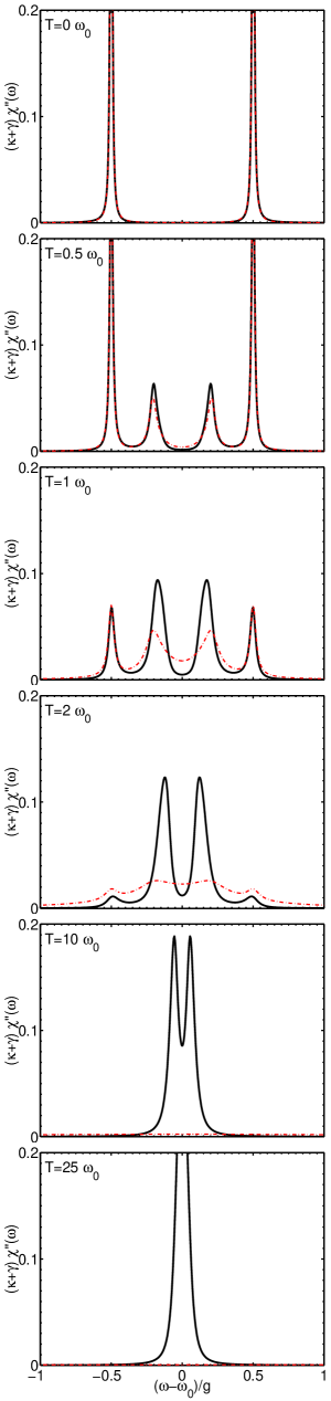
Figure 5: Cavity absorption close to the resonance frequency $\omega_{0}$, for different temperatures. The paramters are taken from Ref. Blais et al., 2004, i.e. qubit-cavity coupling $g=0.01\omega_{0}$, cavity quality factor $Q=10^{4}$, and qubit dissipation $\gamma=0.08\kappa$.

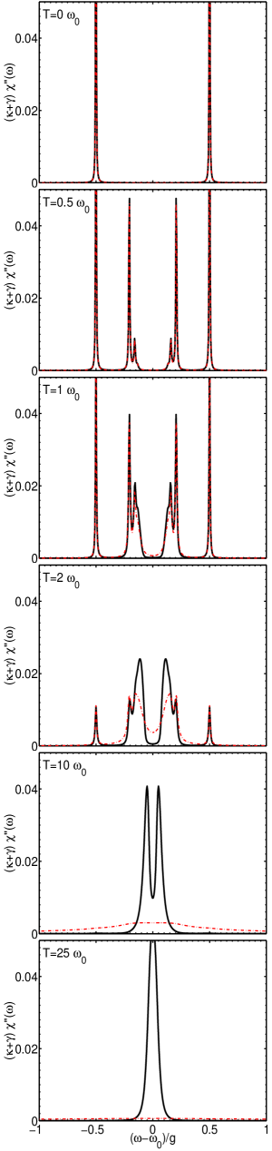
Figure 6: As in Fig. 5 but with improved quality factor of the cavity $Q=10^{5}$ (implies $\gamma=0.8\kappa$).

X Conclusions

In this paper we have studied the regime of cavity QED relevant for the Josephson qubits in superconducting cavities. Namely, we considered the strong coupling regime when the Rabi splitting is much bigger than the inverse life times of the qubit and the cavity, but the temperature is high. This regime may be realized due to the hot photons penetrating the cavity from the manipulating circuits. We have calculated the susceptibility of the cavity and found that it is very sensitive to the temperature. Thus this quantity might be used for temperature measurements. On the formal, theoretical side we noticed that the secular approximation widely used in the applications of the Bloch-Redfield formalism is insufficient when Liouvillian degeneracies are present. We compared solutions found with and without the secular approximation and showed qualitative difference between the two at elevated temperatures.

XI Acknowledgments

We thank R. Schoelkopf, A. Wallraff, E. Il’ichev, P. Zoller, Yu. Makhlin, G. Schön and P. Rabl for fruitful discussions. This work is part of CFN (DFG) and was supported by the Humboldt Foundation, the BMBF and the ZIP programme of the German government, and also by the SQUBIT project of the IST-FET programme of the EC, and by Landesstiftung BW.

References

- Il’ichev et al. (2003) E. Il’ichev, N. Oukhanski, A. Izmalkov, T. Wagner, M. Grajcar, H.-G. Meyer, A. Y. Smirnov, A. Maassen van den Brink, M. H. S. Amin, and A. M. Zagoskin, Phys. Rev. Lett. 91, 097906 (2003).
- Blais et al. (2004) A. Blais, R. S. Huang, A. Wallraff, S. M. Girvin, and R. J. Schoelkopf, cond-mat/0402216 (2004).
- Buisson et al. (2003) O. Buisson, F. Balestro, J. P. Pekola, and F. W. J. Hekking, Phys. Rev. Lett. 90, 238304 (2003).
- Irish and Schwab (2003) E. K. Irish and K. Schwab, Phys. Rev. B 68, 155311 (2003).
- Shore and Knight (1993) B. Shore and P. Knight, J. Mod. Opt. 40, 1195 (1993).
- Thompson et al. (1992) R. J. Thompson, G. Rempe, and H. J. Kimble, Phys. Rev. Lett. 68, 1132 (1992).
- Raimond et al. (2001) J. M. Raimond, M. Brune, and S. Haroche, Rev. Mod. Phys. 73, 565 (2001).
- Cirac et al. (1991) J. I. Cirac, H. Ritsch, and P. Zoller, Phys. Rev. A 44, 4541 (1991).
- Maassen van den Brink and Zagoskin (2002) A. Maassen van den Brink and A. M. Zagoskin, Quant. Inf. Processing 1, 55 (2002).
- Lehmann et al. (2003) J. Lehmann, S. Kohler, P. Hänggi, and A. Nitzan, J. Chem. Phys. 118, 3283 (2003).
- Vion et al. (2002) D. Vion, A. Aassime, A. Cottet, P. Joyez, H. Pothier, C. Urbina, D. Esteve, and M. H. Devoret, Science 296, 886 (2002).
- Feynman and Vernon (1963) R. P. Feynman and F. L. Vernon, Ann. Phys. (NY) 24, 118 (1963).
- Caldeira and Leggett (1981) A. O. Caldeira and A. J. Leggett, Phys. Rev. Lett. 46, 211 (1981).
- Bloch (1957) F. Bloch, Phys. Rev. 105, 1206 (1957).
- Redfield (1957) A. G. Redfield, IBM J. Res. Dev. 1, 19 (1957).