The stochastic dynamics of nanoscale mechanical oscillators immersed in a viscous fluid

Abstract

The stochastic response of nanoscale oscillators of arbitrary geometry immersed in a viscous fluid is studied. Using the fluctuation-dissipation theorem it is shown that deterministic calculations of the governing fluid and solid equations can be used in a straightforward manner to directly calculate the stochastic response that would be measured in experiment. We use this approach to investigate the fluid coupled motion of single and multiple cantilevers with experimentally motivated geometries.

Single molecule force spectroscopy using nanoscale cantilevers immersed in fluid is a tantalizing experimental possibility Viani et al. (1999); Roukes (2000). The precise manner in which nanomechanical devices will be utilized for single-molecule force spectroscopy and sensing is currently under development Arlett et. al. ; Roukes et al. (2000), however the detection system will rely upon the change in response of the cantilever due to the binding of target biomolecules. It is therefore important to build a baseline understanding of the motion of a fluid loaded cantilever, or arrays of cantilevers, in the absence of active molecules. This is the focus of this Letter.

The dynamics of the nanoscale structures considered are dominated by Brownian fluctuations although the mechanical structures are still large compared to the molecular size of the fluid molecules. The elastic response of a single cantilever immersed in fluid has been investigated previously in the context of atomic force microscopy (see for example Sader (1998); Chon et al. (2000)). This theoretical approach, essentially two-dimensional in nature, modelled the cantilever as an infinite cylinder oscillating in an unbounded fluid. This approach has been experimentally validated for long and slender micron-scale cantilevers Chon et al. (2000). However, the response of nanoscale cantilevers (very strong fluidic damping) or short and wide cantilevers (where end effects would be important) is not well understood. Using the fluctuation-dissipation theorem we show that deterministic numerical simulations of the cantilever-fluid system can be used to obtain experimentally relevant stochastic quantities such as the noise spectrum of the fluctuations.

The fluctuation-dissipation theorem allows for the calculation of the equilibrium fluctuations using standard deterministic numerical methods. This is possible because the same molecular processes are responsible for the dissipation and the fluctuations. In the case under consideration here, predominantly these are the collisions of the fluid molecules with the cantilever, although dissipative processes within the elastic material of the cantilever could also be included.

The fluctuation-dissipation theorem comes in many forms. For the fluid-damped motion of nanoscale cantilevers it is sufficient to use a classical formulation. The most convenient form is the one originally discussed by Callen and Greene Callen and Greene (1952) (see also Chandler (1987)). Consider a dynamical variable $A$. For the classical system of interest here this will be a function of the microscopic phase space variables consisting of $3N$ coordinates and conjugate momenta of the cantilever, where $N$ is the number of particles in the cantilever. We investigate the situation where a force $f(t)$ that couples to $A$ is imposed. In this case the Hamiltonian of the system is

$$H=H_{0}-fA$$ (1)

and we look at the linear response for very small $f$. Then it can be shown for the special case of a step function force given by,

$$f(t)=\left\{\begin{array}[c]{cc}F&\text{for }t<0\\ 0&\text{for }t\geq 0\end{array}\right.$$ (2)

that in the linear response regime, the change in the average value of a second dynamical quantity $B$ (again any function of the $3N$ coordinates and momenta) from its equilibrium value in the absence of $f$ is given by

$$\Delta\left\langle B(t)\right\rangle=\beta F\left\langle\delta A(0)\delta B(t)\right\rangle_{0}$$ (3)

where $\beta=(k_{B}T)^{-1}$, $k_{B}$ is Boltzmann’s constant, $T$ is the absolute temperature, $\delta A=A-\left\langle A\right\rangle_{0}$, $\delta B=B-\left\langle B\right\rangle_{0}$ and the subscript zero on the average $\left<\right>$ denotes the equilibrium average in the absence of the force $f$. Thus we can calculate a general equilibrium cross-correlation function in terms of the linear response as

$$\left\langle\delta A(0)\delta B(t)\right\rangle_{0}=k_{B}T\frac{\Delta\left\langle B(t)\right\rangle}{F}.$$ (4)

There are no approximations involved in this result, except that of assuming classical mechanics and linear behavior. If in addition the dynamical variables are sufficiently macroscopic that the mean $\left\langle B(t)\right\rangle$ can be calculated using deterministic, macroscopic equations, we have our desired result.

There are a number of advantages to a formulation of the fluctuation-dissipation theorem in time rather than frequency for our purposes. First, the full correlation function is given by a single (numerical) calculation, the response to removing a step force. The spectral properties can be obtained by Fourier transform. This is particularly advantageous for the low-quality factor ($Q$) situation characteristic of fluid-damped nanoscale cantilevers, since the spectral response is very broad, and a large number of fixed-frequency simulations would be needed to characterize this response. A second advantage is that no expansion in modes of the oscillator is needed. Although such an expansion is not too hard for a high-Q oscillator where the dissipation has negligible influence on the mode shape, for small cantilevers in a fluid, the coupling to the fluid is large, and the motion of the fluid complex, so that a mode analysis would be quite difficult. Finally, the expression Eq. (4) allows us to calculate the correlation function and noise spectrum of precisely the quantity measured in experiment, firstly by tailoring the applied force to couple to one physical variable measured in the experiment ($A$), and then determining the effect on the second physical variable ($B$). This idea has been exploited in the very high-Q situation of the oscillators used in gravitational wave detectors Levin (1998), although there it was convenient to formulate the result in the frequency domain. In our case for example, if the displacement of the cantilever is measured through the strain of a piezoresistive layer near the pivot point Arlett et. al. ; Roukes et al. (2000) of the cantilever, it is possible to tailor the force $F$ to couple to this distortion, and so determine the “strain-strain” correlation function of one or more cantilevers.

Our scheme consists of the following steps in a deterministic simulation: (i) apply the appropriate force $f$, constant in time, small enough so that the response remains linear, and tailored to couple to the variable of interest $A$, and allow the system to come to steady state; (ii) turn off the force at a time we label $t=0$; (iii) measure some dynamical variable $B(t)$ (which might be the same as $A$ to yield an autocorrelation function, or different) to yield the correlation function of the equilibrium fluctuations via Eq. (4). Using the sophisticated numerical tools developed for such calculations, we can find accurate results for realistic experimental geometries that may be quite complex, for example the triangular cantilever design often used in commercial atomic force microscopy, or the reduced stiffness geometries currently under investigation for use as detectors of single biomolecules as shown if Fig. 1.

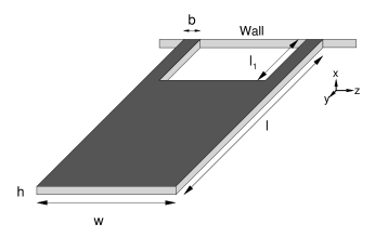
Figure 1: Schematic of the cantilever geometry (not drawn to scale): $l=3\mu$, $w=100$nm, $l_{1}=0.6\mu$, $b=33$nm. The cantilever is silicon with a density $\rho_{s}=2330$Kg/m³, Young’s modulus $E_{s}=125$GPa. This type of geometry is used to reduce the spring constant, the equivalent spring constant $k=8.7$mN/m Arlett et. al. .

For simplicity, we illustrate our approach by finding the auto- and cross-correlation functions for the displacements $x_{i}(t)$ of the tips of one or two nanoscale cantilevers with experimentally realistic geometries. To do this we calculate the deterministic response of the displacement of each tip, which we call $X_{i}(t)$ $i=1,2$, after switching off at $t=0$ a small force applied to the tip of the first cantilever, $F_{1}$, given by Eq. (2). For this case the equilibrium auto- and cross-correlation functions for the fluctuations $x_{1}$ and $x_{2}$ are precisely

$$\left<x_{1}(t)x_{1}(0)\right> = k_{B}TX_{1}(t)/F_{1},$$ (5)

$$\left<x_{2}(t)x_{1}(0)\right> = k_{B}TX_{2}(t)/F_{1}.$$ (6)

The cosine Fourier transform of the auto and cross-correlation functions yield the noise spectrum $G_{11}(\nu)$ and $G_{12}(\nu)$, respectively, which are the experimentally relevant quantities.

We have performed three-dimensional time-dependent numerical simulations of the deterministic fluid-solid coupled problem (algorithm described elsewhere Yang and Makhijani (1994); cfd ). The fluid motion is calculated using the incompressible Navier-Stokes equations and the dynamics of the solid structures are computed from the standard equations of elasticity.

For long ($l\gtrsim 100\mu$) and slender ($l>>w$) cantilevers, the cantilever response can be well approximated as an infinitely long oscillating cylinder Sader (1998); Chon et al. (2000). We first validate our numerical approach by investigating a cantilever in this regime. We emphasize that for the experimentally motivated nanoscale cantilevers of interest here an approximate theory is not available, yet our numerical approach remains valid providing a means to gain valuable insight.

The micron-scale cantilever used for validation has the simple beam geometry as shown in Fig. 2 (b) (see case c2 in Chon et al. (2000)). For micron and nano-scale cantilevers immersed in fluid, dissipation is dominated by the viscous motion of the fluid driven by the cantilever vibrations. This can be described by a Reynolds number based on the frequency of oscillation $\omega$ as $R=\rho\omega w^{2}/4\eta$ where $\rho$ is the fluid density and $\eta$ is the kinematic viscosity. For the cantilevers of interest here the Reynolds numbers are typically $0.01\lesssim R\lesssim 1$ indicating that this is in the low Reynolds number regime. Small $R$ corresponds to strong dissipation.

The noise spectrum, $G_{11}(\nu)$, is calculated from the numerical results by taking the cosine Fourier transform of the autocorrelations and is shown by the solid line in Fig. 2(a). The two broad peaks can be identified with the first two modes of the cantilever. The noise spectrum is also calculated using the long cylinder analytic approximation and is shown by the dashed line. The analytical result for the fundamental mode of the noise spectrum is found in the following manner Sader (1998) (note that higher harmonics could be included if desired). In Fourier space the equation of motion for the cantilever displacement is

$$\left(-m\omega^{2}+k\right)\hat{x}=\hat{F}_{f}+\hat{F}_{B},$$ (7)

where $\hat{F}_{f}$ is the force felt by the cantilever due to the fluid,

$$\hat{F}_{f}=m_{e}\omega^{2}\Gamma(\omega)\hat{x},$$ (8)

$\hat{F}_{B}$ is the fluctuating (Brownian) force, $m_{e}$ is the effective mass  of a fluid cylinder of radius $w/2$, $m$ is the effective mass of the cantilever, and $\Gamma(\omega)$ is the hydrodynamic function (for an infinitely long cylinder of diameter $w$ oscillating in the x-direction) which contains both the fluid damping and fluid loading components and is given by Rosenhead (1963),

$$\Gamma(\omega)=1+\frac{4iK_{1}(-i\sqrt{iR})}{\sqrt{iR}K_{0}(-i\sqrt{iR})}.$$ (9)

where $K_{1}$, $K_{0}$ are Bessel functions and $i=\sqrt{-1}$. From the fluctuation-dissipation theorem the spectral density of the fluctuating force, $G_{F_{B}}(\nu)$, can be related to the dissipation due to the fluid and is given by

$$G_{F_{B}}(\nu)=4k_{B}Tm_{e}T_{0}\omega\Gamma_{i}(\omega),$$ (10)

where $\omega=2\pi\nu$. Solving for the spectral density of the displacement fluctuations, $G_{x}(\nu)$, from Eqs. (7), (8) and (10) yields,

$$G_{x}(\nu)=\frac{4k_{B}T}{k}\frac{1}{\omega_{0}}{\scriptscriptstyle\stackrel{{\scriptstyle\bullet}}{{{}}}}$$

$$\frac{\tilde{\omega}T_{0}\Gamma_{i}(R_{0}\tilde{\omega})}{\left[\left(1-\tilde{\omega}^{2}\left(1+T_{0}\Gamma_{r}(R_{0}\tilde{\omega})\right)\right)^{2}+\left(\tilde{\omega}^{2}T_{0}\Gamma_{i}(R_{0}\tilde{\omega})\right)^{2}\right]}$$

where $\tilde{\omega}=\omega/\omega_{o}$ is the frequency relative to the vacuum resonance frequency $\omega_{0}=\sqrt{k/m}$, $R_{0}$ is the Reynolds number based on $\omega_{0}$, $T_{0}$ is the ratio of the mass of fluid contained in a cylindrical volume of radius $w/2$ to the mass of the cantilever and $\Gamma_{r}$ and $\Gamma_{i}$ are the real and imaginary parts of $\Gamma$, respectively. Sader’s analysis Sader (1998) does not take into account the frequency dependence of the noise force and assumes that the numerator is constant. The frequency dependence is not large for $R\lesssim 1$; however the correction has been included in our analysis. Equation (The stochastic dynamics of nanoscale mechanical oscillators immersed in a viscous fluid) yields the analytical curve for $G_{11}(\nu)$ in Fig. 2(a) and the agreement is excellent with our numerical results.

Figure 2: Panel (a) the noise spectrum from simulation (solid line) and from theory (dashed line). For the theory calculation only the fundamental mode has been considered. Panel (b) is a schematic of the micron-scale cantilever used for validation: length $l=197\mu$, width $w=29\mu$ and height $h=2\mu$. The applied step force is $F_{1}=26$ nN.

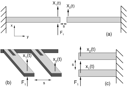
Figure 3: Schematic showing various cantilever configurations. In all configurations the step force $F_{1}$ is released at $t=0$ resulting in the cantilever motion referred to by $X_{1}(t)$. The motion of the neighboring cantilever is, $X_{2}(t)$, and is driven through the response of the fluid. Panel (a) two cantilevers with ends facing, panel (b) side-by-side cantilevers and panel (c) cantilevers separated along the direction of the oscillations

A recent study of the fluid coupled motion of two adjacent $1\mu$ beads illustrates the importance of understanding the cross correlations in the fluctuations for use in single molecule force measurements Meiners and Quake (1999). The fluid disturbance caused by an oscillating cantilever is long range, producing motion of the other cantilevers through the viscous drag. As a result, the stochastic motion of multiple cantilevers will be correlated. However, the numerical approach developed here remains valid for multiple fluid-loaded cantilevers of arbitrary geometry, and our approach can be used to quantify the response of multiple cantilevers with the precise complex geometries used in experiment (as we show below) as well as to help develop a better analytical understanding of idealized geometries. Various possible cantilever configurations are shown in Fig. 3(a)-(c); here we will present results for the end to end case and defer results for the other geometries to a later paper.

Figure 4: Absolute predictions of the auto- and cross-correlation functions of the equilibrium fluctuations of the cantilevers shown in Figs. 1 and 3. Panel (a) a schematic of the step force boundary condition that is applied to the tip of the first cantilever, $F_{1}=75$pN. Panel (b) shows the autocorrelation and panel (c) the cross-correlation of the fluctuations (5 separations are shown $s=h,2h,3h,4h,5h$ where only $s=h,5h$ are labelled and the remaining curves lie between these values in sequential order).

We use our approach to calculate the behavior of the experimentally motivated cantilever shown in Fig. 1. Full three-dimensional simulations were performed for both one cantilever and two cantilevers facing end to end in fluid as shown in Fig. 3(a). Through the fluctuation-dissipation theorem the simulations yield results for the cantilever autocorrelation function and the two cantilever cross-correlation function shown in Fig. 4(b) and (c), respectively. The response of the driven cantilever (on the left) was not significantly affected, for any of the separations investigated, by the presence of the adjacent passive cantilever on the right. The value of $\left<x_{1}(0)x_{1}(0)\right>$ is $0.471\text{nm}^{2}$ indicating that the deflection of the cantilever due to Brownian motion in an experiment would be $0.686\text{nm}$ or about $2.3\%$ of the thickness of the cantilever. The cross-correlation of the Brownian fluctuations of two cantilevers is small compared with the individual fluctuations. The largest magnitude of the of the cross-correlation is $-0.012\text{nm}^{2}$ for $s=h$ and $-0.0029\text{nm}^{2}$ for $s=5h$. The noise spectra for both the one and two cantilever fluctuations, given by the cosine Fourier transform of the cross-correlation function, are shown in Fig. 5(a) and (b). Notice that tuning the separation could be used to reduce the correlated noise in some chosen frequency band.

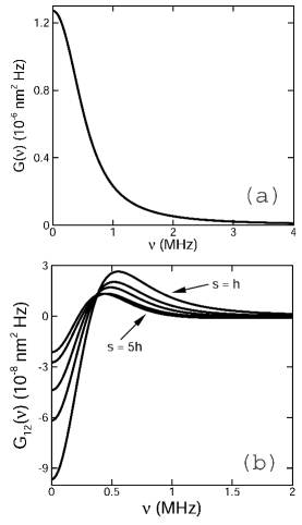
Figure 5: Panel (a): The noise spectrum, $G_{11}(\nu)$. Panel (b): The noise spectrum, $G_{12}(\nu)$, as a function of cantilever separation, $s$, for two adjacent experimentally realistic cantilevers (see Fig. 1). Five separations are shown $s=h,2h,3h,4h,5h$ where only $s=h,5h$ are labelled and the remaining curves lie between these values in sequential order.

The variation in the cross-correlation behavior with cantilever separation as shown in Figure 4(c) can be understood as an inertial effect resulting from the nonzero Reynolds number of the fluid flow, as follows. The flow around the cantilever can be separated into a potential component, which is long range and propagates instantaneously in the incompressible fluid approximation, and a vorticity containing component that propagates diffusively with diffusion constant given by the kinematic viscosity $\nu$. For step forcing, it takes a time $\tau_{v}=s^{2}/\nu$ for the vorticity to reach distance $s$. For small cantilever separations the viscous component dominates, for nearly all times, and results in the anticorrelated response of the adjacent cantilever in agreement with Meiners and Quake (1999). However, as $s$ increases the amount of time where the adjacent cantilever is only subject to the potential flow field increases resulting in the initial correlated behavior.

In summary, a numerical approach to calculate the stochastic response of single and multiple nanocantilevers, of arbitrary geometry, immersed in a viscous fluid using deterministic calculations has been developed, validated, and applied to an experimentally relevant cantilever geometry. The methods described here are applicable to atomic force microscopy in general and also to other nano-structure fluid interaction problems which are of growing importance as NEMS technology advances.

This research was carried out within the Caltech BioNEMS effort (M.L. Roukes, PI), supported by DARPA/MTO Simbiosys under grant F49620-02-1-0085. We gratefully acknowledge extensive interactions with this team. MP thanks the Burroughs Wellcome Foundation ”Interfaces” program for additional support.

References

- Viani et al. (1999) M. B. Viani, T. E. Schäffer, and A. Chand, J. Appl. Phys. 86, 2258 (1999).
- Roukes (2000) M. L. Roukes, Nanoelectromechanical systems, condmat/0008187 (2000).
- (3) J. Arlett et. al., to be published.
- Roukes et al. (2000) M. Roukes, S. Fraser, M. Cross, and J. Solomon, Active nems arrays for biochemical analyses, U.S. Patent App. No. 60/224,109 (2000).
- Sader (1998) J. E. Sader, J. Appl. Phys. 84, 64 (1998).
- Chon et al. (2000) J. W. M. Chon, P. Mulvaney, and J. Sader, J. Appl. Phys. 87, 3978 (2000).
- Callen and Greene (1952) H. B. Callen and R. F. Greene, Phys. Rev. 86, 702 (1952).
- Chandler (1987) D. Chandler, Introduction to modern statistical mechanics (Oxford University Press, 1987).
- Levin (1998) Y. Levin, Phys. Rev. D 57, 659 (1998).
- Yang and Makhijani (1994) H. Yang and V. Makhijani, AIAA-94-0179 pp. 1–10 (1994).
- (11) CFD Research Corporation, 215 Wynn Dr. Huntsville AL 35805.
- Rosenhead (1963) L. Rosenhead, Laminar boundary layers (Oxford, 1963).
- Meiners and Quake (1999) J.-C. Meiners and S. R. Quake, Phys. Rev. Lett. 82, 2211 (1999).