$1/f$ Noise in a one-dimensional charge density wave system

Abstract

The current noise in a classical one-dimensional charge density wave system is studied in the weak pinning regime by solving the overdamped equation of motion numerically. At low temperatures and just above the zero temperature depinning threshold, the power spectrum of the current noise $S(f)$ was found to scale with frequency $f$ as $S(f)\sim f^{-\gamma}$, where $\gamma\approx 1$, suggesting the existence of flicker noise. Our result is in agreement with experimental findings for quasi-one-dimensional charge density wave systems and provides the first evidence of $1/f$ behavior obtained from first principles.

I Introduction

The noise in any system is characterized in terms of the shape of its spectral power density $S(f)$, which may be measured directly in experiments. If $S(f)\sim f^{-\gamma}$ and $\gamma\approx 1$, then such a noise is referred to as $1/f$ or flicker noise. Its existence has attracted the attention of researchers from various branches of the natural sciences for many years. As for physical systems, $1/f$ noise has been observed as fluctuations in the currents of diodes, vacuum tubes and transistors, the resistance of carbon microphones, metallic thin films and semiconductors Voss79 ; Hooge76 ; Bochkov83 , the magnetization in spin glasses Reim86 and in many other systems.

Despite a substantial amount of experimental and theoretical effort, a unique underlying mechanism for the flicker noise remains unknown and still poses an open question as to its universal origins Milotti01 ; Sethna01 ; Antal01 . However, there is now increasing evidence that the non-trivial exponent, at least in electronic systems, may come from equilibrium dynamics in the presence of disorder Kogan96 when energy barriers exceed the typical thermal energy.

$1/f^{\gamma}$ noise in charge density wave (CDW) systems Gruner88 has been studied mainly in NbSe₃ and TaS₃ materials Kogan96 . The first experiment was done on a bulk NbSe₃ sample by Richard et al. Richard82 who found $\gamma\sim 0.8$. Studying transport properties of the quasi-one-dimensional CDW material TaS₃ at low temperatures, Zaitsev–Zotov Zaitsev93 observed that slightly above the depinning threshold of the driving electric field, the exponent $\gamma$ for the current noise is equal to $\gamma\approx 1.2$.

It should be noted that a phenomenological model based on fluctuations in impurity pinning force due to deformations of the sliding condensate was proposed to explain the broad band $1/f$ noise in CDW systems Bhattacharya85 . However, neither theoretical nor numerical estimation of $\gamma$ has been provided so far. The aim of the present paper is to compute $\gamma$ from first principles with the help of a one-dimensional classical model for CDWs Gorkov77 . The current was obtained through numerical simulation of the overdamped equation of motion. The $1/f$ scaling is evaluated using the so-called Wavelet Transform Modulus Maxima (WTMM) method Arneodo . The exponent $\gamma$ was found to depend on $T$. At low temperatures ($T\leq 0.1$), in agreement with the experiments Zaitsev93 , we obtain $\gamma\approx 1.2$ in the crossover regime. Exponent $\gamma$ drops with increasing $T$ and the ”exact” $1/f$-noise is observed at $T\approx 0.3$ where $\gamma$ becomes 1. This interesting result is indicative of the possible occurrence of $1/f$ noise. At high temperatures $\gamma$ takes on the white noise value 0.

Notably, the observed $\gamma\approx 1$ is not related to the second order depinning transition behavior at $T=0$. Due to the asymptotic uniqueness of the sliding state Middleton92 , this critical point dynamics scenario leads to the ‘trivial’ exponent $\gamma\approx 2$ Narayan92 ; Fisher98 . Additionally, the observed ‘flicker’ noise behavior $\gamma\approx 1$ gains on its scaling range with increased distance to the critical point of the second order depinning transition.

Based on unusual current–voltage characteristics Zaitsev93 ; Zaitsev94 ; Zaitsev97a ; Zaitsev97b , Zaitsev-Zotov suggested that at low temperatures the quantum creep dynamics may play an important role and proposed the crossover from classical to quantum creep regime as an alternative explanation for experimental results. The strength of the quantum fluctuations in 1D CDW systems can be estimated by a dimensionless parameter $K$ GlaNa02 which is proportional to $\sqrt{m^{*}/m}$, where $m^{*}$ is the effective band mass. This quantity is of the order $10^{-2}$ to $10^{-1}$ Maki95 ; Gruner88 , indicating irrelevance (to 1/f noise) of quantum effects at low temperatures. Furthermore, our simulation results on transport properties Glatz02 also suggest, in comparison to experiments, that quantum fluctuations do not have any visible effect with respect to the strength of the driving forces under consideration (see also discussion in Kiss88 ; Handel88 ). On the other hand, due to the small parameter $K$ the core action of phase slips in the bulk is large ($S_{\textit{core}}\propto 1/K$) GlaNa02 and hence the probability of phase slips which are proportional to $e^{-S_{\textit{core}}}$ becomes small. It decreases even more under a renormalization group transformation, such that we can neglect phase slips in our simulations. Therefore we will use the one-dimensional classical model without phase slips to study the current noise in CDW systems.

II Model

The charge–density $\rho(x)$ of an 1D CDW can be expressed as $\rho(x)=\rho_{0}(1+Q^{-1}\partial_{x}\varphi(x))+\rho_{1}\cos{\big{(}Qx+\varphi(x)\big{)}}$, where $Q=2k_{F}$ denotes the wave vector of the undistorted wave, $k_{F}$ the Fermi wave vector and $\varphi(x)$ a slowly varying phase variable. $\rho_{0}=Q/\pi$ is the mean electron density and $\rho_{1}$ is proportional to the amplitude of the complex order parameter GlaNa02 . The Hamiltonian of the phase field is then given by

$${\cal H}=\int dx\,\Bigg{\{}\frac{c}{2}\left(\frac{\partial}{\partial x}\varphi\right)^{2}-\sum\limits_{i}V_{i}\delta(x-x_{i})\times\rho_{1}\cos{\big{(}Qx+\varphi(x)\big{)}}+Ex\partial_{x}\varphi(x)\Bigg{\}}\,,$$ (1)

where $c=\frac{\hbar v_{F}}{2\pi}$ is the elastic constant with the Fermi–velocity $v_{F}$, and $V_{i}$ and $x_{i}$ denote the strength and the position of the impurity potential acting on the CDW, respectively; $E$ is the external electric field or driving force.

Our numerical studies are done in the weak pinning limit, i.e. when the Fukuyama–Lee length FuLee78 $L_{c}=(c/V)^{2/3}$ is large compared to the mean impurity distance $l_{\textit{imp}}$. Therefore we will restrict ourselves in the following to the case $L_{c}\gg l_{\textit{imp}}\gg Q^{-1}$, where the full Hamiltonian (1) can be reduced to a random field XY–model:

$${\cal H}=\int dx\left\{\frac{c}{2}\left(\frac{\partial}{\partial x}\varphi\right)^{2}\right.\left.-V\cos{\big{(}\varphi-\alpha(x)\big{)}}\,-\,E\varphi(x)\right\}\,.$$ (2)

Here $\alpha(x)$ is a random phase with zero average and $\overline{e^{i\big{(}\alpha(x)-\alpha(x^{\prime})\big{)}}}=\delta(x-x^{\prime})$, where the overbar denotes the averaging over disorder realizations. $V$ is defined by $\overline{(V_{i}\rho_{1})(V_{j}\rho_{1})}\equiv V^{2}\delta_{ij}$ ($\overline{V_{i}}=0$). The equation of motion of the (overdamped) CDW is given by a Langevin equation

$$\frac{\partial\varphi}{\partial t}=-\gamma\frac{\delta{\cal H}}{\delta\varphi}+\eta(x,t)\,,$$ (3)

where $\gamma$ is a kinetic coefficient and $\eta(x,t)$ a Gaussian thermal noise characterized by $\big{<}\eta\big{>}=0$ and $\big{<}\eta(x,t)\,\eta(x^{\prime},t^{\prime})\big{>}=2T\gamma\,\delta(x-x^{\prime})\,\delta(t-t^{\prime})$.

The length scale $L_{c}$ sets an energy scale $T^{\ast}=\left(c^{\phantom{1}}V^{2}\right)^{1/3}=c^{\phantom{1}}L_{c}^{-1}$. We will rescale time by $L_{c}/\gamma T^{\ast}$, temperature by $T^{\ast}$, and the external field $E$ by $E^{\ast}$, where $E^{\ast}=T^{\ast}/L_{c}$ is of the order of the $T=0$ depinning threshold field $E_{c}$. In the following, $E$ denotes the rescaled and dimensionless quantity.

Solving the discretized version of Eq. 3 one can find he time dependent current $j_{\textit{cdw}}(t)$ which is defined as Glatz01

$$j_{\textit{cdw}}(t)=\overline{\left\langle\frac{\partial\varphi(x,t)}{\partial t}\right\rangle_{x}},$$ (4)

where $\left\langle...\right\rangle_{x}$ denotes the average over positions.

III Simulation

The effect of disorder on the dynamical behavior of the one-dimensional charge density wave model (2) at low temperatures was studied Glatz01 with the help of the discretized version of equation (3) and it was found that, contrary to high dimensional systems Natter90 , the dependency of the creep velocity on the electric field is described by an analytic function. The current noise spectrum was not, however, explored. Following Ref. Glatz01 , the equation of motion (3) is integrated by a modified Runge–Kutta algorithm suitable for stochastic systems with periodic boundary conditions.

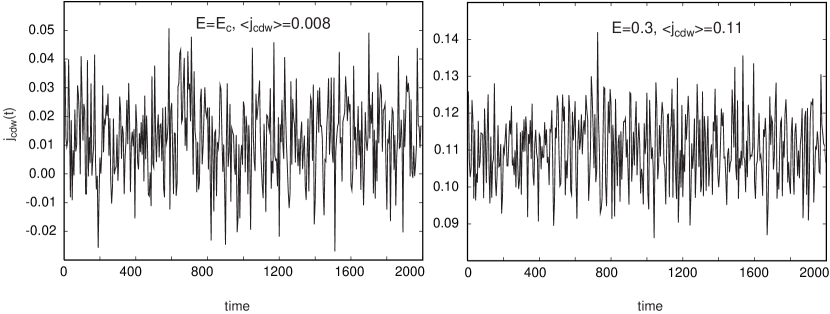
Figure 1: Typical time dependence of the CDW current for $E=E_{c}=0.22$ (left panel) and $E=0.3$ (right panel) at $T=0.1$ for one disorder realization. The time and disorder averaged values of $j_{\textit{cdw}}(t)$ are shown next to the curves ($\langle j_{\textit{cdw}}\rangle$). We took $N=5000$ and the results are averaged over 1000 and 500 samples for $E=E_{c}$ and $E=0.3$, respectively. An initial (dimensionless) time interval of length $\approx 2000$ is discarded, such that the system is in the steady state at time $0$.

Throughout this paper, we use a system size of $N=5000$ and average the results over typically $N_{s}=1000$ disorder realizations. Larger system sizes do not change the results substantially. Fig. 1 shows the typical time evolution of $j_{\textit{cdw}}(t)$ for $E=E_{c}=0.22$ Glatz01 (upper panel) and $E=0.3$ (lower panel) at temperature $T=0.1$. One can see that the current exhibits strong fluctuations. The time averaged values are $\langle j_{\textit{cdw}}\rangle=0.008\pm 0.003$ and $\langle j_{\textit{cdw}}\rangle=0.112\pm 0.006$ for $E=E_{c}$ and $E=0.3$, respectively. The spike structure is also seen, but less pronounced compared to the experimental data Zaitsev93 . Nevertheless, the patterns for the two values of $E$ look similar.

Zaitsev–Zotov studied Zaitsev93 the current noise spectrum for applied electric fields with averaged driving current $\left\langle I\right\rangle\geq 220$pA. Using Fig. 1 from Ref. Zaitsev93 one can see that the threshold electric field in these experiments is $E_{c}\approx 35$V/cm and the averaged currents of $\left\langle I\right\rangle=220$pA and $\left\langle I\right\rangle=2.4$nA at $T=2.4$K correspond to electric fields $E\approx 40$V/cm and $E\approx 50$V/cm, respectively, i.e. the electric fields used are greater than the threshold field. Therefore we will restrict our spectrum analysis to $E\geq E_{c}$.

IV Scaling exponent estimation

It should be noted that in the case of non-stationary behavior of the CDW current as in our simulations, the standard Fourier transformation is not suitable for determining the exponent $\gamma$ and one should, therefore, employ more sophisticated methods. We have chosen the WTMM method Arneodo for its superior properties in non-parametric scaling exponent estimation Audit02 in the presence of polynomial non-stationarities. In particular, attempts to reduce the non-stationary behavior of the current by discarding an initial time interval (as in 1) cannot generally guarantee reaching a steady state, since the relaxation time to a steady state can be very long (see the remark in Ref. Middleton93 ).

The ability of the wavelet transform to provide unbiased scaling estimates of non-stationary signals is due to the property of orthogonality to polynomials up to the degree $n$ of the base functions, of the so-called analyzing wavelets $\psi$ with $m$ ‘vanishing moments’:

$$\int_{-\infty}^{+\infty}x^{n}\,\psi(x)\,dx=0\hskip 14.45377pt\forall n,\;0\leq n<m\;.$$

The transform is defined as the inner product of the function $f(x)$ and the dilated and translated wavelet $\psi(x)$:

$$(Wf)(s,b)=\frac{1}{s}\;\int dx\;f(x)\;\psi(\frac{x-b}{s})\;,$$ (5)

where $s,b\in\mathbb{R}$ and $s>0$ for the continuous version (CWT), which among other properties ensures local blindness to the polynomial bias. Indeed, the wavelet transform decomposes the signal into scale (and thus frequency) dependent components (scale and position localized wavelets), comparable to frequency localized sines and cosines based Fourier decomposition, but with added position localization. This localization in both space and frequency, together with the wavelet’s orthogonality to polynomial bias, makes it possible to access even weak scaling behavior of singularities $h(x_{0})$, otherwise masked by the stronger polynomial components:

$$f(x)_{x_{0}}=c_{0}+c_{1}(x-x_{0})+\dots+c_{n}(x-x_{0})^{m}+C|x-x_{0}|^{h(x_{0})}\;,$$

where function $f$ is represented through its Taylor expansion around $x=x_{0}$.

In the generic multifractal formulation of the WTMM formalism Arneodo , the moments $q$ of the measure distributed on the WTMM tree are taken to obtain the dependency of the scaling function $\tau(q)$ on the moments $q$:

$${\cal Z}(s,q)\sim s^{\tau(q)},$$

where ${\cal Z}(s,q)$ is the partition function of the $q$-th moment of the measure distributed over the wavelet transform maxima at the scale $s$ considered:

$${{\cal Z}(s,q)=\sum_{{\Omega}(s)}(Wf\omega_{i}(s))^{q}\;,}$$ (6)

with ${\Omega}(s)=\{\omega_{i}(s)\}$ as the set of maxima $\omega_{i}(s)$ at the scale $s$ of the continuous wavelet transform $Wf(s,t)$ of the function $f(t)$, in our case the CDW current; $f(t)=j_{\textit{cdw}}(t)$.

In particular, scaling analysis with WTMM is capable of revealing the modal exponent $h(q=0)$ for which the spectrum reaches maximum value; this $h(q=0)$ corresponds to the Hurst exponent $H$ in the case of monofractal noise. This exponent is directly linked to the power spectrum exponent of the (stationary) fluctuations of the analyzed signal by: $\gamma=2H+1$, the relation which links the spectral exponent $\gamma$ with the Hurst exponent $H$.

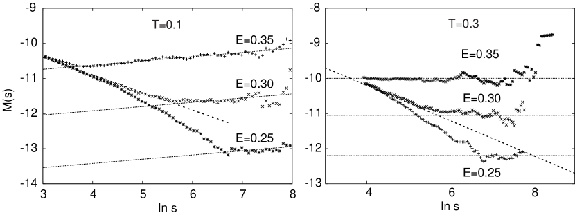
Figure 2: Left: M(s) versus $\ln s$ for the CDW current $j_{\textit{cdw}}(t)$ averaged over $N_{s}=1000$ disorder realizations and for three values of the external electric field: $E=0.25$, 0.3 and 0.35 which are higher than $E_{c}\approx 0.22$. The dotted straight lines denote the reference slope corresponding to $\gamma~{}=~{}1.2$. The dashed line has the slope $-0.5$, which corresponds to the flat power spectrum of white noise $\gamma=0$. Right: The same but for $T=0.3$. The dotted lines denote the reference slope $H=0$ corresponding to $\gamma~{}=~{}1.0$. Again, the dashed line corresponds to white noise.

In Fig. 2, the modal scaling exponent has been obtained by a linear fit over an appropriate scaling range from a suitably defined, weighted measure ${\cal M}(s)$ on the WTMM:

$$h(q=0)=\left.\frac{d\tau(q)}{dq}\right|_{q=0}=\lim_{s\rightarrow 0}\;\frac{{\cal M}(s)}{\log(s)}$$ (7)

with

$${{\cal M}(s)=\frac{\sum_{{\Omega}(s)}\log(Wf\omega_{i}(s))\;,}{{\cal Z}(s,0)}}\;,$$ (8)

and for three electric field values $E$=0.25, 0.3 and 0.35, and for the number of the disorder averaging ensemble fixed to $N_{s}=1000$. Consistent with the experimental findings Zaitsev93 , the flicker noise region becomes narrower with decreasing $E$. More importantly, we obtain $\gamma\approx 1.2$ as observed in experiments Zaitsev93 . Asymptotic transition to the scaling regime characteristic to uncorrelated behavior (white noise, i.e., $\gamma=0$) can be clearly identified for all the values of $E$ shown (see dashed line in Fig. 2).

Fig. 2) (right) shows M(s) versus $\ln s$ for $j_{\textit{cdw}}(t)$ for three values of the external electric field $E=0.25$, 0.3 and 0.35 and $T=0.3$. Our fitting gives $\gamma=1$, which is important from the point of view of the exact definition of $1/f$-noise. In Fig. 3, we provide the dependence of the exponent $\gamma$ on temperature. Note the convergence towards $\gamma=1.2$ as the temperature (and the averaged current) approaches 0. The exponent $\gamma$ decays quickly with temperature and we have the uncorrelated noise value $\gamma=0$ at high $T$.

The primary question remaining is that of the origins of $1/f$ noise in the CDW system. In our opinion, the disorder causes the rugged energy landscape (similar to the spin glass case) leading to a wide spectrum of relaxation times. The average over such a spectrum would give rise to the flicker noise Bochkov83 . Our results shown in Fig. 3 support this point of view. Namely, at low temperatures the roughness of the energy landscape becomes more important and consequently the flicker-like regime occurs. Another qualitative scenario Milotti01 for the appearance of the flicker noise in our system is that the CDW may be viewed as a single particle in a quasi-periodic potential with troughs of variable depths. Such a simplified model closely resembles the “many-pendula” model of the self-organized criticality Bak87 in which the $1/f$ noise should occur.

Figure 3: The dependence of the exponent $h(q=0)$ on temperature. Note the convergence towards $H=0.1$ corresponding with $\gamma=1.2$ spectral exponent for $0$ values of temperature and current.

V Conclusion

In conclusion, using the classical one-dimensional CDW model and multifractal analysis, we have reproduced the experimental results on the current noise spectrum. Our simulations support the existence of $1/f$-noise in this system. To the best of our knowledge, this is the first evidence of $1/f$ scaling obtained from first principle based simulation in a physical (i.e. CDW) system.

It would be interesting to check if a three-dimensional version of our model gives $\gamma\approx 0.8$ obtained for the bulk NbSe₃ sample Richard82 or if other models should be implemented to reproduce this experimental result. The effect of higher dimensionalities, phase slips and quantum fluctuations on the flicker noise remains a challenge for future studies.

VI Acknowledgement

The authors wish to thank A. Ausloos, J. Kertesz, T. Nattermann, S. Scheidl and S. Zaitsev–Zotov for useful discussions. AG acknowledges financial support from the Deutsche Forschungsgemeinschaft through Sonderforschungsbereich 608 and the Deutscher Akademischer Austauschdienst and MS Li from the Polish agency KBN.

References

- (1) R. F. Voss, Proc. 33rd Annu. Symp. Frequency Contr. , Atlantic City, NJ, 1979, p. 40.
- (2) F. N. Hooge, Physica B 83, 14 (1976)
- (3) G. N. Bochkov and Yu. E. Kuzovlev, Sov. Phys.-Usp. 26, 829 (1983).
- (4) A.A. Middleton and D.S. Fischer, Phys. Rev. B 47, 3530 (1993).
- (5) W. Reim, R. H. Koch, A. P. Malozemoff, and M. B. Ketchen, Phys. Rev. Lett. 57, 905 (1996)
- (6) E. Milotti, physics/0204033 (2001).
- (7) J.P. Sethna, K.A. Dahmen, and C.R. Myers, Nature 410, 242 (2001).
- (8) T. Antal, M. Droz, G. Gyorgyi, Z. Racz, Phys. Rev. Lett. 87, 240601 (2001).
- (9) Sh. Kogan, Electronic noise and fluctuations in solids, Cambridge, University Press, 1996
- (10) G. Grüner, Rev. Mod. Phys. 60, 1128 (1988).
- (11) J. Richard et al,J. Phys. C: Solid State Phys. 15, 7157 (1982).
- (12) S.V. Zaitsev-Zotov, Phys. Rev. Lett. 71, 605 (1993).
- (13) S. Bhattacharya em et al., Phys. Rev. Lett. 54, 2453 (1985).
- (14) L.P. Gorkov, JETP Lett. 25, 358 (1977).
- (15) A. Arneodo, E. Bacry and J.F. Muzy, Physica A, 213, 232 (1995). J.F. Muzy, E. Bacry, and A. Arneodo, Int. J. of Bifurcation and Chaos 4, No. 2, 245 (1994).
- (16) A. A. Middleton, Phys. Rev. Lett. 68, 670 (1992).
- (17) O. Narayan, D.S. Fisher, Phys. Rev. B 46, 11520 (1992).
- (18) D.S. Fisher, Phys. Rep. 301, 113 (1998).
- (19) S.V. Zaitsev-Zotov, Phys. Rev. Lett. 72, 587 (1994).
- (20) S.V. Zaitsev-Zotov, G. Remenyi, and P. Monceau, Phys. Rev. B 56, 6388 (1997).
- (21) S.V. Zaitsev-Zotov, G. Remenyi, and P. Monceau, Phys. Rev. Lett. 78, 1098 (1997).
- (22) A. Glatz and T. Nattermann, Phys. Rev. Lett. 88, 256401 (2002); cond-mat/0310432.
- (23) K. Maki, Phys. Lett. A 202, 313 (1995).
- (24) A. Glatz, Z. R. Struzik, and M. S. Li, preprint.
- (25) L.B. Kiss, Reviews of Solid State Science, 2, 569 (1988).
- (26) P.H. Handel, J. Phys. C, 21, 2435 (1988)
- (27) H. Fukuyama and P. A. Lee, Phys. Rev. B 17, 535 (1978).
- (28) A. Glatz, S. Kumar, and M. S. Li, Phys. Rev. B 64 184301 (2001).
- (29) T. Nattermann, Phys. Rev. Lett 64, 2454 (1990).
- (30) B. Audit, J.F. Muzy, A. Arneodo, to appear in IEEE, Trans. in Information Theory (2002).
- (31) P. Bak, C. Tang, and K. Wiesenfeld, Phys. Rev. Lett. 59, 381 (1987).