Strongly Correlated Electron Materials:
Dynamical Mean-Field Theory
and Electronic Structure

Abstract

These are introductory lectures to some aspects of the physics of strongly correlated electron systems. I first explain the main reasons for strong correlations in several classes of materials. The basic principles of dynamical mean-field theory (DMFT) are then briefly reviewed. I emphasize the formal analogies with classical mean-field theory and density functional theory, through the construction of free-energy functionals of a local observable. I review the application of DMFT to the Mott transition, and compare to recent spectroscopy and transport experiments. The key role of the quasiparticle coherence scale, and of transfers of spectral weight between low- and intermediate or high energies is emphasized. Above this scale, correlated metals enter an incoherent regime with unusual transport properties. The recent combinations of DMFT with electronic structure methods are also discussed, and illustrated by some applications to transition metal oxides and f-electron materials.

1 Introduction: why strong correlations ?

1.1 Hesitant electrons: delocalised waves or localised particles ?

The physical properties of electrons in many solids can be described, to a good approximation, by assuming an independent particle picture. This is particularly successful when one deals with broad energy bands, associated with a large value of the kinetic energy. In such cases, the (valence) electrons are highly itinerant: they are delocalised over the entire solid. The typical time spent near a specific atom in the crystal lattice is very short. In such a situation, valence electrons are well described using a wave-like picture, in which individual wavefunctions are calculated from an effective one-electron periodic potential.

For some materials however, this physical picture suffers from severe limitations and may fail altogether. This happens when valence electrons spend a larger time around a given atom in the crystal lattice, and hence have a tendency towards localisation. In such cases, electrons tend to “see each other” and the effects of statistical correlations between the motions of individual electrons become important. An independent particle description will not be appropriate, particularly at short or intermediate time scales (high to intermediate energies). A particle-like picture may in fact be more appropriate than a wave-like one over those time scales, involving wavefunctions localised around specific atomic sites. Materials in which electronic correlations are significant are generally associated with moderate values of the bandwidth (narrow bands). The small kinetic energy implies a longer time spent on a given atomic site. It also implies that the ratio of the Coulomb repulsion energy between electrons and the available kinetic energy becomes larger. As a result delocalising the valence electrons over the whole solid may become less favorable energetically. In some extreme cases, the balance may even become unfavorable, so that the corresponding electrons will remain localised. In a naive picture, these electrons sit on the atoms to which they belong and refuse to move. If this happens to all the electrons close to the Fermi level, the solid becomes an insulator. This insulator is difficult to understand in the wave-like language: it is not caused by the absence of available one-electron states caused by destructive interference in ${\bf k}$-space, resulting in a band-gap, as in conventional band insulators. It is however very easy to understand in real space (thinking of the solid as made of individual atoms pulled closer to one another in order to form the crystal lattice). This mechanism was understood long ago Mott (1949, 1990) by Mott (and Peierls), and such insulators are therefore called Mott insulators (Sec. 4. In other cases, such as f-electron materials, this electron localisation affects only part of the electrons in the solid (e.g the ones corresponding to the f-shell), so that the solid remains a (strongly correlated) metal.

The most interesting situation, which is also the one which is hardest to handle theoretically, is when the localised character on short time-scales and the itinerant character on long time-scales coexist. In such cases, the electrons “hesitate” between being itinerant and being localised. This gives rise to a number of physical phenomena, and also results in several possible instabilities of the electron gas which often compete, with very small energy differences between them. In order to handle such situations theoretically, it is necessary to think both in ${\bf k}$-space and in real space, to handle both the particle-like and the wave-like character of the electrons and, importantly, to be able to describe physical phenomena on intermediate energy scales. For example, one needs to explain how long-lived (wave-like) quasiparticles may eventually emerge at low energy/temperature in a strongly correlated metal while at higher energy/temperature, only incoherent (particle-like) excitations are visible. It is the opinion of the author that, in many cases, understanding these intermediate energy scales and the associated coherent/incoherent crossover is the key to the intriguing physics often observed in correlated metals. In these lectures, we discuss a technique, the dynamical mean-field theory (DMFT), which is able to (at least partially) handle this problem. This technique has led to significant progress in our understanding of strong correlation physics, and allows for a quantitative description of many correlated materialsGeorges et al. (1996); T.Pruschke et al. (1995). Extensions and generalisations of this technique are currently being developed in order to handle the most difficult/mysterious situations which cannot be tamed by the simplest version of DMFT.

1.2 Bare energy scales

Localised orbitals and narrow bands

In practice, strongly correlated materials are generally associated with partially filled d- or f- shells. Hence, the suspects are materials involving:

• Transition metal elements (particularly from the 3d-shell from Ti to Cu, and to a lesser extent 4d from Zr to Ag).

• Rare earth (4f from Ce to Yb) or actinide elements (5f from Th to Lw)

To this list, one should also add molecular (organic) conductors with large unit cell volumes in which the overlap between molecular orbitals is weak.

What is so special about d- and f- orbitals (particularly 3d and 4f) ? Consider the atomic wavefunctions of the 3d shell in a 3d transition metal atom (e.g Cu). There are no atomic wavefunctions with the same value $l=2$ of the angular momentum quantum number, but lower principal quantum number $n$ than $n=3$ (since one must have $l\leq\,n-1$). Hence, the 3d wavefunctions are orthogonal to all the $n=1$ and $n=2$ orbitals just because of their angular dependence, and the radial part needs not have nodes or extend far away from the nucleus. As a result, the 3d-orbital wave functions are confined more closely to the nucleus than for s or p states of comparable energy. The same argument applies to the 4f shell in rare earths. It also implies that the 4d wavefunctions in the 4d transition metals or the 5f ones in actinides will be more extended (and hence that these materials are expected to display, on the whole, weaker correlation effects than 3d transition metals, or the rare earth, respectively).

Oversimplified as it may be, these qualitative arguments at least tell us that a key energy scale in the problem is the degree of overlap between orbitals on neighbouring atomic sites. This will control the bandwidth and the order of magnitude of the kinetic energy. A simple estimate of this overlap is the matrix element:

$$t\,_{{\bf R}{\bf R}^{\prime}}^{LL^{\prime}}\,\sim\,\int d{\bf r}\,\chi^{*}_{L}({\bf r}-{\bf R})\,\frac{\hbar^{2}\nabla^{2}}{2m}\,\chi_{L^{\prime}}({\bf r}-{\bf R}^{\prime})$$ (1)

In the solid, the wavefunction $\chi_{L}({\bf r}-{\bf R})$ should be thought of as a Wannier-like wave function centered on atomic site ${\bf R}$. In narrow band systems, typical values of the bandwith are a few electron-volts.

Coulomb repulsion and the Hubbard $U$

Another key parameter is the typical strength of the Coulomb repulsion between electrons sitting in the most localized orbitals. The biggest repulsion is associated with electrons with opposite spins occupying the same orbital: this is the Hubbard repulsion which we can estimate as:

$$U\,\sim\,\int d{\bf r}d{\bf r}^{\prime}|\chi_{L}({\bf r}-{\bf R})|^{2}\,U_{s}({\bf r}-{\bf r}^{\prime})\,|\chi_{L}({\bf r}^{\prime}-{\bf R})|^{2}$$ (2)

In this expression, $U_{s}$ is the interaction between electrons including screening effects by other electrons in the solid. Screening is a very large effect: if we were to estimate (2) with the unscreened Coulomb interaction $U({\bf r}-{\bf r}^{\prime})=e^{2}/|{\bf r}-{\bf r}^{\prime}|$, we would typically obtain values in the range of tens of electron-volts. Instead, the screened value of $U$ in correlated materials is typically a few electron-volts. This can be comparable to the kinetic energy for narrow bandwiths, hence the competition between localised and itinerant aspects. Naturally, other matrix elements (e.g between different orbitals, or between different sites) are important for a realistic description of materials (see the last section of these lectures).

In fact, a precise description of screening in solids is a rather difficult problem. An important point is, again, that this issue crucially depends on energy scale. At very low energy, one should observe the fully screened value, of order a few  eV ’s, while at high energies (say, above the plasmon energy in a metal) one should observe the unscreened value, tens of  eV ’s. Indeed, the screened effective interaction $W({\bf r},{\bf r}^{\prime};\omega)$ as estimated e.g from the RPA approximation, is a strong function of frequency (see e.g Ref. Springer and Aryasetiawan (1998); Aryasetiawan et al. (2004) for an ab-initio GW treatment in the case of Nickel). As a result, using an energy-independent parametrization of the on-site matrix elements of the Coulomb interaction such as (2) can only be appropriate for a description restricted to low- enough energies Aryasetiawan et al. (2004). The Hubbard interaction can only be given a precise meaning in a solid, over a large enery range, if it is made energy-dependent. I shall come back to this issue in the very last section of these lectures (Sec. 5.5).

The simplest model hamiltonian

From this discussion, it should be clear that the simplest model in which strong correlation physics can be discussed is that of a lattice of single-level “atoms”, or equivalently of a single tight-binding band (associated with Wannier orbitals centered on the sites of the crystal lattice), retaining only the on-site interaction term between electrons with opposite spins:

$$H=-\sum_{{\bf R}{\bf R}^{\prime},\sigma}t_{{\bf R}{\bf R}^{\prime}}\,c^{+}_{{\bf R}\sigma}c_{{\bf R}^{\prime}\sigma}\,+\,\varepsilon_{0}\sum_{{\bf R}\sigma}n_{{\bf R}\sigma}\,+\,U\sum_{{\bf R}}n_{{\bf R}\uparrow}n_{{\bf R}\downarrow}$$ (3)

The kinetic energy term is diagonalized in a single-particle basis of Bloch’s wavefunctions:

$$H_{0}=\sum_{{\bf k}\sigma}\varepsilon_{\bf k}c^{+}_{{\bf k}\sigma}c_{{\bf k}\sigma}\,\,\,;\,\,\,\varepsilon_{\bf k}\equiv\sum_{{\bf R}^{\prime}}\,t_{{\bf R}{\bf R}^{\prime}}\,e^{i{\bf k}\cdot({\bf R}-{\bf R}^{\prime})}$$ (4)

with e.g for nearest-neighbour hopping on the simple cubic lattice in d-dimensions:

$$\varepsilon_{\bf k}\,=\,-2t\sum_{\mu=1}^{d}\cos(k_{\mu}a)$$ (5)

In the absence of hopping, we have, at each site, a single atomic level and hence four possible quantum states: $|\,0\rangle,|\,\uparrow\rangle,|\,\downarrow\rangle$ and $|\,\uparrow\downarrow\rangle$ with energies $0\,,\,\varepsilon_{0}$ and $U+2\varepsilon_{0}$, respectively.

Eq. (3) is the famous Hubbard model Hubbard (1963, 1964a, 1964b). It plays in this field the same role than that played by the Ising model in statistical mechanics: a laboratory for testing physical ideas, and theoretical methods alike. Simplified as it may be, and despite the fact that it already has a 40-year old history, we are far from having explored all the physical phenomena contained in this model, let alone of being able to reliably calculate with it in all parameter ranges !

1.3 Examples of strongly correlated materials

In this section, I give a few examples of strongly correlated materials. The discussion emphasizes a few key points but is otherwise very brief. There are many useful references related to this section, e.g Varma and Giamarchi (1991); Imada et al. (1998); Mott (1990); Tsuda et al. (2000); Harrison (1989).

1.3.1 Transition metals

In 3d transition metals, the 4s orbitals have lower energy than the 3d and are therefore filled first. The 4s orbitals extend much further from the nucleus, and thus overlap strongly. This holds the atoms sufficiently far apart so that the d- orbitals have a small direct overlap. Nevertheless, d-orbitals extend much further from the nucleus than the “core” electrons (corresponding to shells which are deep in energy below the Fermi level). As a result, throughout the 3d series of transition metals (and even more so in the 4d series), d-electrons do have an itinerant character, giving rise to quasiparticle bands. That this is the case is already clear from a very basic property of the material, namely how the equilibrium unit- cell volume depends on the element as one moves along the 3d series (Fig. 1). The unit-cell volume has a very characteristic, roughly parabolic, dependence. A simple model of a narrow band being gradually filled, introduced long ago by Friedel Friedel (1969) accounts for this parabolic dependence (see also McMahan et al. (1998); Wills and Eriksson (2000)). Because the states at the bottom of the band are bonding-like while the states at the top of the band are anti-bonding like, the binding energy is maximal (and hence the equilibrium volume is minimal) for a half-filled shell. Instead, if the d-electrons were localised we would expect little contribution of the d-shell to the cohesive energy of the solid, and the equilibrium volume should not vary much along the series.

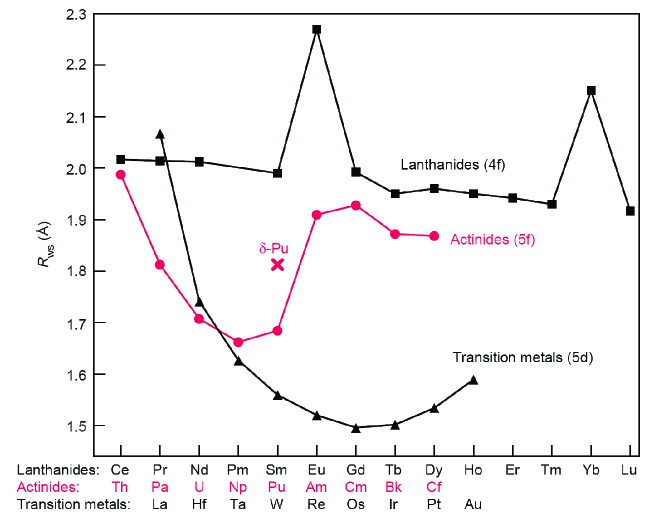
Figure 1: Experimental Wigner-Seitz Radius of Actinides, Lanthanides, and 5d Transition Metals. The equilibrium volume of the primitive unit cell is given by $V=4\pi\,R_{WS}^{3}/3$. Elements that lie on top of each other have the same number of valence electrons. The volume of the transition metals has a roughly parabolic shape, indicating delocalised 5d electrons. The volumes of the lanthanides remain roughly constant, indicating localised 4f electrons. The volumes of the light actinides decrease with increasing atomic number, whereas the volumes of the late actinides behaves similarly to that of the lanthanides. From Ref. Wills and Eriksson (2000)

Screening is relatively efficient in transition metals because the 3d band is not too far in energy from the 4s band. The latter plays the dominant role in screening the Coulomb interaction (crudely speaking, one has to consider the following charge transfer process between two neighbouring atoms: $3d^{n}4s+3d^{n}4s\rightarrow 3d^{n-1}4s^{2}+3d^{n+1}$, see e.g Anisimov and Gunnarsson (1991) for further discussion). For all these reasons (the band not being extremely narrow, screening being efficient), electron correlations do have important physical effects for 3d transition metals, but not extreme ones like localisation. Magnetism of these metals below the Curie temperature, but also the existence of fluctuating local moments in the paramagnetic phase are exemples of such correlation effects. Band structure calculations based on DFT-LDA methods overestimate the width of the occupied d-band (by about 30% in the case of nickel). Some features observed in spectroscopy experiments (such as the (in)famous 6 eV satellite in nickel) are also signatures of correlation effects, and are not reproduced by standard electronic structure calculations.

1.3.2 Transition metal oxides

In transition metal compounds (e.g oxides or chalcogenides), the direct overlap between d-orbitals is generally so small that d-electrons can only move through hybridisation with the ligand atoms (e.g oxygen 2p-bands). For example, in the cubic perovskite structure shown on Fig. 2, each transition-metal atom is “encaged” at the center of an octahedron made of six oxygen atoms. Hybridisation leads to the formation of bonding and antibonding orbitals. An important energy scale is the charge-transfer energy $\Delta=\varepsilon_{d}-\varepsilon_{p}$, i.e the energy difference between the average position of the oxygen and transition metal bands. When $\Delta$ is large as compared to the overlap integral $t_{pd}$, the bonding orbitals have mainly oxygen character and the antibonding ones mainly transition-metal character. In this case, the effective metal- to- metal hopping can be estimated as $t_{eff}\sim\,t_{pd}^{2}/\Delta$, and is therefore quite small.

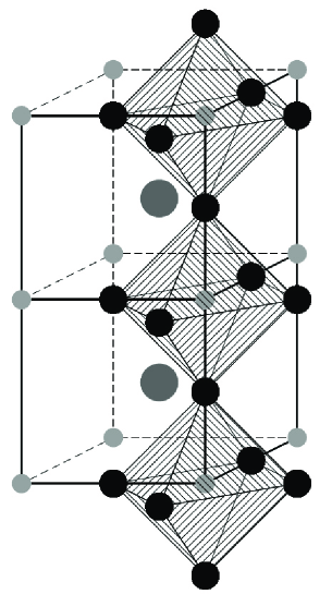
Figure 2: The cubic perovskite structure, e.g of the compound SrVO₃ . Transition-metal atoms (V) - small grey spheres- are at the center of oxygen octahedra (dark spheres). Sr atoms are the larger spheres in-between planes. From Ref. Maiti (1997).

The efficiency of screening in transition-metal oxides depends crucially on the relative position of the 4s and 3d band. For 3d transition metal monoxides MO with M to the right of Vanadium, the 4s level is much higher in energy than 3d, thus leading to poor screening and large values of $U$. This, in addition to the small bandwidth and relatively large $\Delta$, leads to dramatic correlation effects, turning the system into a Mott insulator (or rather, a charge- transfer insulator, see below), in spite of the incomplete filling of the d-band. The Mott phenomenon plays a key role in the physics of transition- metal oxides, as discussed in detail later in these lectures (see Sec. 4 and Fig. 6).

Crystal field splitting

The 5-fold (10-fold with spin) degeneracy of the d- orbitals in the atom is lifted in the solid, due to the influence of the electric field created by neighbouring atoms, i.e the ligand oxygen atoms in transition metal oxides. For a transition metal ion in an octahedral environment (as in Fig. 2), this results in a three-fold group of states ($t_{2g}$) which is lower in energy and a doublet ($e_{g}$) higher in energy. Indeed, the $d_{xy},d_{yz},d_{zx}$ orbitals forming the $t_{2g}$ multiplet do not point towards the ligand atoms, in contrast to the states in the $e_{g}$ doublet ($d_{x^{2}-y^{2}}$, $d_{3z^{2}-r^{2}}$). The latter therefore lead to a higher cost in Coulomb repulsion energy. For a crystal with perfect cubic symmetry, the $t_{2g}$ and $e_{g}$ multiplets remain exactly degenerate, while a lower symmetry of the crystal lattice lifts the degeneracy further. For a tetrahedral environment of the transition-metal ion, the opposite situation is found, with $t_{2g}$ higher in energy than $e_{g}$. In transition metals, the energy scale associated with crystal- field splitting is typically much smaller than the bandwith. This is not so in transition-metal oxides, for which these considerations become essential. In some materials, such as e.g SrVO₃  and the other $d^{1}$ oxides studied in Sec. 5.3 of these lectures, the energy bands emerging from the $t_{2g}$ and $e_{g}$ orbitals form two groups of bands well separated in energy.

Mott- and charge-transfer insulators

There are two important considerations, which are responsible for the different physical properties of the “early” (i.e involving Ti, V, Cr, …) and “late” (Ni, Cu) transition- metal oxides:

- whether the Fermi level falls within the $t_{2g}$ or $e_{g}$ multiplets,

- what is the relative position of oxygen ($\varepsilon_{p}$) and transition-metal ($\varepsilon_{p}$) levels ?

For those compounds which correspond to an octahedral environment:

• In early transition-metal oxides, $t_{2g}$ is partially filled, $e_{g}$ is empty. Hence, the hybridisation with ligand is very weak (because $t_{2g}$ orbitals point away from the 2p oxygen orbitals). Also, the d-orbitals are much higher in energy than the 2p orbitals of oxygen. As a result, the charge-transfer energy $\Delta=\varepsilon_{d}-\varepsilon_{p}$ is large, and the bandwidth is small. The local d-d Coulomb repulsion $U_{dd}$ is a smaller scale than $\Delta$ but it can be larger than the bandwidth ($\sim t_{pd}^{2}/\Delta$): this leads to Mott insulators.

• For late transition-metal oxides, $t_{2g}$ is completely filled, and the Fermi level lies within $e_{g}$. As a result, hybridisation with the ligand is stronger. Also, because of the greater electric charge on the nuclei, the attractive potential is stronger and as a result, the Fermi level moves closer to the energy of the 2p ligand orbitals. Hence, $\Delta$ is a smaller scale than $U_{dd}$ and controls the energy cost of adding an extra electron. When this cost becomes larger than the bandwidth, insulating materials are obtained, often called “charge transfer insulators” Fujimori and Minami (1984); Zaanen et al. (1985). The mechanism is not qualitatively different than the Mott mechanism, but the insulating gap is set by the scale $\Delta$ rather than $U_{dd}$ and separates the oxygen band from a d-band rather than a lower and upper Hubbard bands having both d-character.

The p-d model

The single-band Hubbard model is easily extended in order to take into account both transition-metal and oxygen orbitals in a simple modelisation of transition-metal oxides. The key terms to be retained are:

$$H_{pd}=-\sum_{{\bf R}{\bf R}^{\prime},\sigma}t_{pd}\,(d^{+}_{{\bf R}\sigma}p_{{\bf R}^{\prime}\sigma}+h.c)\,+\,\varepsilon_{d}\sum_{{\bf R}\sigma}n^{d}_{{\bf R}\sigma}+\varepsilon_{p}\sum_{{\bf R}^{\prime}\sigma}n^{p}_{{\bf R}^{\prime}\sigma}\,+\,U_{dd}\sum_{{\bf R}}n^{d}_{{\bf R}\uparrow}n^{d}_{{\bf R}\downarrow}$$ (6)

to which one may want to add other terms, such as: Coulomb repulsions $U_{pp}$ and $U_{pd}$ or direct oxygen-oxygen hoppings $t_{pp}$.

1.3.3 f-electrons: rare earths, actinides and their compounds

A distinctive character of the physics of rare-earth metals (lanthanides) is that the 4f electrons tend to be localised rather than itinerant (at ambiant pressure). As a result, the f-electrons contribute contribute little to the cohesive energy of the solid, and the unit-cell volume depends very weakly on the filling of the 4f shell (Fig. 1). Other electronic orbitals do form bands which cross the Fermi level however, hence the metallic character of the lanthanides. When pressure is applied, the f-electrons become increasingly itinerant. In fact, at some critical pressure, some rare-earth metals (mots notably Ce and Pr) undergo a sharp first-order transition which is accompanied by a discontinuous drop of the equilibrium unit-cell volume. Cerium is a particularly remarkable case, with a volume drop of as much as $15\%$ and the same crystal symmetry (fcc) in the low-volume ($\alpha$) and high-volume ($\gamma$) phase. In other cases, the transition corresponds to a change in crystal symmetry, from a lower symmetry phase at low pressure to a higher symmetry phase at high pressure. For a recent review on the volume-collapse transition of rare earth metals, see Ref. McMahan et al. (1998).

The equilibrium volume of actinide (5f) metals display behaviour which is intermediate between transition metals and rare earths. From the beginning of the series (Th) until Plutonium (Pu), the volume has an approximately parabolic dependence on the filling of the f-shell, indicating delocalised 5f electrons. From Americium onwards, the volume has a much weaker dependence on the number of f-electrons, suggesting localised behaviour. Interestingly, plutonium is right on the verge of this delocalisation to localisation transition. Not surprisingly then, plutonium is, among all actinide metals, the one which has the most complex phase diagram and which is also the most difficult to describe using conventional electronic structure methods (see Wills and Eriksson (2000); Kotliar and Savrasov (2003) for recent reviews). This will be discussed further in the last section of these lectures. This very brief discussion of rare-earths and actinide compounds is meant to illustrate the need for methods able to deal simultaneously with the itinerant and localised character of electronic degrees of freedom.

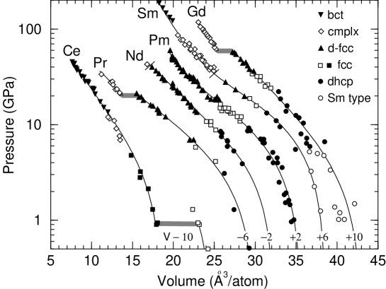
Figure 3: Pressure volume data for the rare earths. Structures are identified, with “cmplx” signifiying a number of complex, low-symmetry structures. The volume collapse transitions are marked by the wide hatched lines for Ce, Pr, and Gd, while lines perpendicular to the curves denote the d-fcc to hP3 symmetry change in Nd and Sm. The curves are guides to the eye. Note that the data and curves have been shifted in volume by the numbers (in ų/atom) shown at the bottom of the figure. Figure and caption reproduced from Ref. McMahan et al. (1998).

The physics of strong electronic correlations becomes even more apparent for f-electron materials which are compounds involving rare-earth (or actinide) ions and other atoms, such as e.g CeAl₃ . A common aspect of such compounds is the formation of quasiparticle bands with extremely large effective masses (and hence large values of the low-temperature specific heat coefficient $\gamma=C/T$), up to a thousand time the bare electron mass ! Hence the term “heavy-fermion” given to these compounds: for reviews, see e.g Coleman (2002); Hewson (1993). The origin of these large effective masses is the weak hybridization between the very localised f-orbitals and the rather broad conduction band associated with the metallic ion. At high temperature/energy, the f-electron have localised behaviour (yielding e.g local magnetic moments and a Curie law for the magnetic susceptibility). At low temperature/energy, the conduction electrons screen the local moments, leading to the formation of quasiparticle bands with mixed f- and conduction electron character (hence a large Fermi surface encompassing both f- and conduction electrons). The low-temperature susceptibility has a Pauli form and the low-energy physics is, apart from some specific compounds, well described by Fermi liquid theory. This screening process, the Kondo effect, is associated with a very low energy coherence scale, the (lattice Burdin et al. (2000)-) Kondo temperature, considerably renormalised as compared to the bare electronic energy scales.

The periodic Anderson model

The simplest model hamiltonian appropriate for f-electron materials is the Anderson lattice or periodic Anderson model. It retains the f-orbitals associated with the rare-earth or actinide atoms at each lattice site, as well as the relevant conduction electron degrees of freedom which hybridise with those orbitals. In the simplest form, the hamiltonian reads:

$$H_{PAM}\,=\,\sum_{{\bf k}\sigma}\varepsilon_{\bf k}\,c^{\dagger}_{{\bf k}\sigma}c_{{\bf k}\sigma}\,+\,\sum_{{\bf k}\sigma\,m}(V_{{\bf k}}\,c^{\dagger}_{{\bf k}\sigma}f_{m{\bf k}\sigma}+h.c\,)+\,\varepsilon_{f}\sum_{{\bf R}\sigma\,m}\,n^{f}_{{\bf R}\sigma\,m}\,+\,U\,\sum_{{\bf R}}\left(\sum_{\sigma\,m}n^{f}_{{\bf R}\sigma\,m}\right)^{2}$$ (7)

Depending on the material considered, other terms may be necessary for increased realism, e.g an orbital dependent f-level $\varepsilon_{fm}$, hybridisation $V_{{\bf k}\,m}$ or interaction matrix $U_{mm^{\prime}}^{\sigma\sigma^{\prime}}$ or a direct f-f hopping $t_{ff}$.

2 Dynamical Mean-Field Theory at a glance

Dealing with strong electronic correlations is a notoriously difficult theoretical problem. From the physics point of view, the difficulties come mainly from the wide range of energy scales involved (from the bare electronic energies, on the scale of electron-Volts, to the low-energy physics on the scale of Kelvins) and from the many competing orderings and instabilities associated with small differences in energy.

It is the opinion of the author that, on top of the essential guidance from physical intuition and phenomenology, the development of quantitative techniques is essential in order to solve the key open questions in the field (and also in order to provide a deeper understanding of some “classic” problems, only partially understood to this day).

In this section, we explain the basic principles of Dynamical Mean-Field Theory (DMFT). This approach has been developed over the last fifteen years and has led to some significant advances in our understanding of strong correlations. In this section, we explain the basic principles of this approach in a concise manner. The Hubbard model is taken as an example. For a much more detailed presentation, the reader is referred to the available review articles Georges et al. (1996); T.Pruschke et al. (1995).

2.1 The mean-field concept, from classical to quantum

Mean-field theory approximates a lattice problem with many degrees of freedom by a single-site effective problem with less degrees of freedom. The underlying physical idea is that the dynamics at a given site can be thought of as the interaction of the local degrees of freedom at this site with an external bath created by all other degrees of freedom on other sites (Fig. 4).

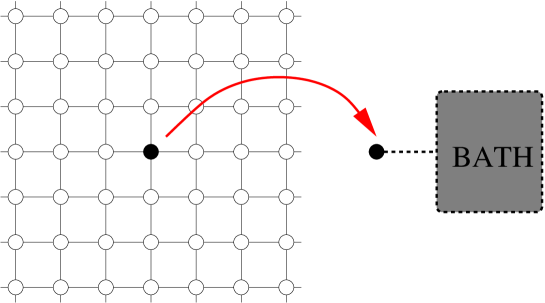
Figure 4: Mean-field theory replaces a lattice model by a single site coupled to a self-consistent bath.

Classical mean-field theory

The simplest illustration of this idea is for the Ising model:

$$H=-\sum_{(ij)}J_{ij}S_{i}S_{j}-h\,\sum_{i}S_{i}$$ (8)

Let us focus on the thermal average of the magnetization on each lattice site: $m_{i}=\langle S_{i}\rangle$. We consider an equivalent problem of independent spins:

$$H_{eff}=-\sum_{i}h^{eff}_{i}\,S_{i}$$ (9)

in which the (Weiss) effective field is chosen in such a way that the value of $m_{i}$ is accurately reproduced. This requires:

$$\beta h^{eff}_{i}=\tanh^{-1}m_{i}$$ (10)

Let us consider, for definiteness, a ferromagnet with nearest-neighbour couplings $J_{ij}=J\,>0$. The mean-field theory approximation (first put forward by Pierre Weiss, under the name of “molecular field theory”) is that $h_{i}^{eff}$ can be approximated by the thermal average of the local field seen by the spin at site $i$, namely:

$$h_{i}^{eff}\simeq h+\sum_{j}J_{ij}\,m_{j}=h+zJm$$ (11)

where $z$ is the connectivity of the lattice, and translation invariance has been used ($J_{ij}=J$ for n.n sites, $m_{i}=m$). This leads to a self-consistent equation for the magnetization:

$$m\,=\,\mbox{tanh}\,(\beta h+z\beta Jm)$$ (12)

We emphasize that replacing the problem of interacting spins by a problem of non-interacting ones in a effective bath is not an approximation, as long as we use this equivalent model for the only purpose of calculating the local magnetizations. The approximation is made when relating the Weiss field to the degrees of freedom on neighbouring sites, i.e in the self-consistency condition (11). We shall elaborate further on this point of view in the next section, where exact energy functionals will be discussed. The mean-field approximation becomes exact in the limit where the connectivity $z$ of the lattice becomes large. It is quite intuitive indeed that the neighbors of a given site can be treated globally as an external bath when their number becomes large, and that the spatial fluctuations of the local field become negligible.

Generalisation to the quantum case: dynamical mean-field theory

This construction can be extended to quantum many-body systems. Key steps leading to this quantum generalisation where: the introduction of the limit of large lattice coordination for interacting fermion models by Metzner and Vollhardt Metzner and Vollhardt (1989) and the mapping onto a self-consistent quantum impurity by Georges and Kotliar Georges and Kotliar (1992), which established the DMFT framework.

I explain here the DMFT construction on the simplest example of the Hubbard model:

$$H=-\sum_{ij,\sigma}t_{ij}\,c^{\dagger}_{i\sigma}c_{j\sigma}+U\sum_{i}n_{i\uparrow}n_{i\downarrow}+\varepsilon_{0}\,\sum_{i\sigma}n_{i\sigma}$$ (13)

As explained above, it describes a collection of single-orbital “atoms” placed at the nodes ${\bf R}_{i}$ of a periodic lattice. The orbitals overlap from site to site, so that the fermions can hop with an amplitude $t_{ij}$. In the absence of hopping, each “atom” has 4 eigenstates: $|0\rangle,|\uparrow\rangle,|\downarrow\rangle$ and $\uparrow\downarrow\rangle$ with energies $0\,,\,\varepsilon_{0}$ and $U+2\varepsilon_{0}$, respectively.

The key quantity on which DMFT focuses is the local Green’s function at a given lattice site:

$$G^{\sigma}_{ii}(\tau-\tau^{\prime})\,\equiv\,-\langle Tc_{i\sigma}(\tau)c^{\dagger}_{i\sigma}(\tau^{\prime})\rangle$$ (14)

In classical mean-field theory, the local magnetization $m_{i}$ is represented as that of a single spin on site $i$ coupled to an effective Weiss field. In a completely analogous manner, we shall introduce a representation of the local Green’s function as that of a single atom coupled to an effective bath. This can be described by the hamiltonian of an Anderson impurity model :

$$H_{AIM}=H_{atom}+H_{bath}+H_{coupling}$$ (15)

in which:

$$H_{atom}=U\,n^{c}_{\uparrow}n^{c}_{\downarrow}+(\varepsilon_{0}-\mu)\,(n^{c}_{\uparrow}+n^{c}_{\downarrow})$$

$$H_{bath}=\sum_{l\sigma}\widetilde{\epsilon}_{l}\,a^{\dagger}_{l\sigma}a_{l\sigma}$$

$$H_{coupling}=\sum_{l\sigma}V_{l}\,(a^{\dagger}_{l\sigma}c_{\sigma}+c^{\dagger}_{\sigma}a_{l\sigma})$$ (16)

In these expressions, a set of non-interacting fermions (described by the $a^{\dagger}_{l}$’s) have been introduced, which are the degrees of freedom of the effective bath acting on site ${\bf R}_{i}$. The $\widetilde{\epsilon}_{l}$ and $V_{l}$’s are parameters which should be chosen in such a way that the c-orbital (i.e impurity) Green’s function of (16) coincides with the local Green’s function of the lattice Hubbard model under consideration. In fact, these parameters enter only through the hybridisation function:

$$\Delta(i\omega_{n})=\sum_{l}\frac{|V_{l}|^{2}}{i\omega_{n}-\widetilde{\epsilon}_{l}}$$ (17)

This is easily seen when the effective on-site problem is recast in a form which does not explicitly involves the effective bath degrees of freedom. However, this requires the use of an effective action functional integral formalism rather than a simple hamiltonian formalism. Integrating out the bath degrees of freedom one obtains the effective action for the impurity orbital only under the form:

$$S_{eff}=-\int^{\beta}_{0}d\tau\int^{\beta}_{0}d\tau^{\prime}\,\sum_{\sigma}c^{+}_{\sigma}(\tau){\cal G}_{0}^{-1}(\tau-\tau^{\prime})c_{\sigma}(\tau^{\prime})+U\,\int^{\beta}_{0}d\tau\,n_{\uparrow}(\tau)n_{\downarrow}(\tau)$$ (18)

in which:

$${\cal G}_{0}^{-1}(i\omega_{n})=i\omega_{n}+\mu-\varepsilon_{0}-\Delta(i\omega_{n})$$ (19)

This local action represents the effective dynamics of the local site under consideration: a fermion is created on this site at time $\tau$ (coming from the ”external bath”, i.e from the other sites of the lattice) and is destroyed at time $\tau^{\prime}$ (going back to the bath). Whenever two fermions (with opposite spins) are present at the same time, an energy cost $U$ is included. Hence this effective action describes the fluctuations between the 4 atomic states $|0\rangle,|\uparrow\rangle,|\downarrow\rangle,\uparrow\downarrow\rangle$ induced by the coupling to the bath. We can interpret ${\cal G}_{0}(\tau-\tau^{\prime})$ as the quantum generalisation of the Weiss effective field in the classical case. The main difference with the classical case is that this “dynamical mean-field” is a function of energy (or time) instead of a single number. This is required in order to take full account of local quantum fluctuations, which is the main purpose of DMFT. ${\cal G}_{0}$ also plays the role of a bare Green’s function for the effective action $S_{eff}$, but it should not be confused with the non-interacting ($U=0$) local Green’s function of the original lattice model.

At this point, we have introduced the quantum generalisation of the Weiss effective field and have represented the local Green’s function $G_{ii}$ as that of a single atom coupled to an effective bath. This can be viewed as an exact representation, as further detailed in Sec. 3. We now have to generalise to the quantum case the mean-field approximation relating the Weiss function to $G_{ii}$ (in the classical case, this is the self-consistency relation (12)). The simplest manner in which this can be explained - but perhaps not the more illuminating one conceptually (see Sec. 3 and Georges et al. (1996); Georges (2002))- is to observe that, in the effective impurity model (18), we can define a local self-energy from the interacting Green’s function $G(\tau-\tau^{\prime})\equiv-<Tc(\tau)c^{+}(\tau^{\prime})>_{S_{eff}}$ and the Weiss dynamical mean-field as:

$$\Sigma_{imp}(i\omega_{n})\,\equiv {\cal G}_{0}^{-1}(i\omega_{n})-G^{-1}(i\omega_{n})$$

$$= i\omega_{n}+\mu-\varepsilon_{0}-\Delta(i\omega_{n})-G^{-1}(i\omega_{n})$$ (20)

Let us, on the other hand, consider the self-energy of the original lattice model, defined as usual from the full Green’s function $G_{ij}(\tau-\tau^{\prime})\equiv-<Tc_{i,\sigma}(\tau)c_{j,\sigma}^{+}(\tau^{\prime})>$ by:

$$G({{\bf k}},i\omega_{n})\,=\,\frac{1}{i\omega_{n}+\mu-\epsilon_{0}-\epsilon_{{\bf k}}-\Sigma({\bf k},i\omega_{n})}$$ (21)

in which $\epsilon_{{\bf k}}$ is the Fourier transform of the hopping integral, i.e the dispersion relation of the non-interacting tight-binding band:

$$\epsilon_{{\bf k}}\equiv\sum_{j}t_{ij}e^{i{\bf k}.({\bf R}_{i}-{\bf R}_{j})}$$ (22)

We then make the approximation that the lattice self-energy coincides with the impurity self-energy. In real-space, this means that we neglect all non-local components of $\Sigma_{ij}$ and approximate the on-site one by $\Sigma_{imp}$:

$$\Sigma_{ii}\simeq\Sigma_{imp}\,\,\,,\,\,\,\Sigma_{i\neq j}\simeq 0$$ (23)

We immediately see that this is a consistent approximation only provided it leads to a unique determination of the local (on-site) Green’s function, which by construction is the impurity-model Green’s function. Summing (21) over ${\bf k}$ in order to obtain the on-site component $G_{ii}$ of the the lattice Green’s function, and using (20), we arrive at the self-consistency condition:

$$\sum_{{\bf k}}\frac{1}{\Delta(i\omega_{n})+G(i\omega_{n})^{-1}-\varepsilon_{\bf k}}\,=\,G(i\omega_{n})$$ (24)

Defining the non-interacting density of states:

$$D(\varepsilon)\,\equiv\,\sum_{\bf k}\,\delta(\varepsilon-\varepsilon_{\bf k})$$ (25)

this can also be written as:

$$\int d\varepsilon\,\frac{D(\varepsilon)}{\Delta(i\omega_{n})+G(i\omega_{n})^{-1}-\varepsilon}\,=\,G(i\omega_{n})$$ (26)

This self-consistency condition relates, for each frequency, the dynamical mean-field $\Delta(i\omega_{n})$ and the local Green’s function $G(i\omega_{n})$. Furthermore, $G(i\omega_{n})$ is the interacting Green’s function of the effective impurity model (16) -or (18)-. Therefore, we have a closed set of equations that fully determine in principle the two functions $\Delta,G$ (or ${\cal G}_{0}$,$G$)). In practice, one will use an iterative procedure, as represented on Fig. 5. In many cases, this iterative procedure converges to a unique solution independently of the initial choice of $\Delta(i\omega_{n})$. In some cases however, more than one stable solution can be found (e.g close to the Mott transition, see section below). The close analogy between the classical mean-field construction and its quantum (dynamical mean-field) counterpart is summarized in Table 1.

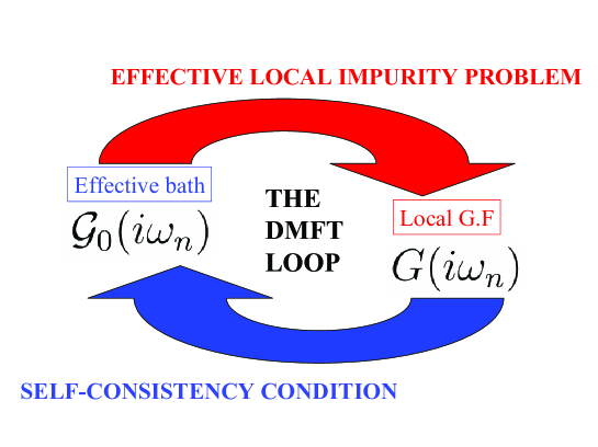
Figure 5: The DMFT iterative loop. The following procedure is generally used in practice: starting from an initial guess for ${\cal G}_{0}$, the impurity Green’s function $G_{imp}$ is calculated by using an appropriate solver for the impurity model (top arrow). The impurity self-energy is also calculated from $\Sigma_{imp}={\cal G}_{0}^{-1}(i\omega_{n})-G_{imp}^{-1}(i\omega_{n})$. This is used in order to obtain the on-site Green’s function of the lattice model by performing a ${\bf k}$-summation (or integration over the free d.o.s): $G_{loc}=\sum_{\bf k}[i\omega_{n}+\mu-\varepsilon_{\bf k}-\Sigma_{imp}(i\omega_{n})]^{-1}$. An updated Weiss function is then obtained as ${\cal G}_{0,new}^{-1}=G_{loc}^{-1}+\Sigma_{imp}$, which is injected again into the impurity solver (bottom arrow). The procedure is iterated until convergence is reached.

Quantum Case	Classical Case
$-\sum_{ij\sigma}t_{ij}c^{+}_{i\sigma}c_{j\sigma}+\sum_{i}H_{atom}(i)$	$H=-\sum_{(ij)}J_{ij}S_{i}S_{j}-h\sum_{i}S_{i}$	Hamiltonian
$G_{ii}(i\omega_{n})=-<c^{+}_{i}(i\omega_{n})c_{i}(i\omega_{n})>$	$m_{i}=<S_{i}>$	Local Observable
$H_{eff}=H_{atom}+\sum_{l\sigma}\widetilde{\epsilon}_{l}a^{+}_{l\sigma}a_{l\sigma}+$	$H_{eff}=-h_{eff}\,S$	Effective single-site
$+\sum_{l\sigma}V_{l}(a^{+}_{l\sigma}c_{\sigma}+h.c)$		Hamiltonian
$\Delta\,(i\omega_{n})=\sum_{l}\frac{|V_{l}|^{2}}{i\omega_{n}-\widetilde{\epsilon}_{l}}$	$h_{eff}$	Weiss function/Weiss field
${\cal G}_{0}^{-1}(i\omega_{n})\equiv i\omega_{n}+\mu-\Delta(i\omega_{n})$
$\sum_{{\bf k}}[\Delta(i\omega_{n})+G(i\omega_{n})^{-1}-\epsilon_{{\bf k}}]^{-1}=G(i\omega_{n})$	$h_{eff}=\sum_{j}J_{ij}m_{j}+h$	Self-consistency relation

Table 1: Correspondance between the mean-field theory of a classical system and the dynamical mean-field theory of a quantum system.

2.2 Limits in which DMFT becomes exact

Two simple limits: non-interacting band and isolated atoms

It is instructive to check that the DMFT equations yield the exact answer in two simple limits:

• In the non-interacting limit $U=0$, solving (18) yields $G(i\omega_{n})={\cal G}_{0}(i\omega_{n})$ and $\Sigma_{imp}=0$. Hence, from (24), $G(i\omega_{n})=\sum_{\bf k}1/(i\omega_{n}+\mu-\varepsilon_{0}-\varepsilon_{\bf k})$ reduces to the free on-site Green’s function. DMFT is trivially exact in this limit since the self-energy is not only ${\bf k}$-independent but vanishes altogether.

• In the atomic limit $t_{ij}=0$, one just has a collection of independent atoms on each site and $\varepsilon_{\bf k}=0$. Then (24) implies $\Delta(i\omega_{n})=0$: as expected, the dynamical mean-field vanishes since the atoms are isolated. Accordingly, the self-energy only has on-site components, and hence DMFT is again exact in this limit. The Weiss field reads ${\cal G}_{0}^{-1}=i\omega_{n}+\mu-\varepsilon_{0}$, which means that the action $S_{eff}$ simply corresponds to the quantization of the atomic hamiltonian $H_{atom}$. This yields:

  $$G(i\omega_{n})_{atom}=\frac{1-n/2}{i\omega_{n}+\widetilde{\mu}}+\frac{n/2}{i\omega_{n}+\widetilde{\mu}-U}$$

  $$\Sigma(i\omega_{n})_{atom}=\frac{nU}{2}+\frac{n/2(1-n/2)U^{2}}{i\omega_{n}+\widetilde{\mu}-(1-n/2)U}$$ (27)

  with $\widetilde{\mu}\equiv\mu-\varepsilon_{0}$ and $n/2=(e^{\beta\widetilde{\mu}}+e^{\beta(2\widetilde{\mu}-U)})/(1+2e^{\beta\widetilde{\mu}}+e^{\beta(2\widetilde{\mu}-U)})$.

Hence, the dynamical mean-field approximation is exact in the two limits of the non-interacting band and of isolated atoms, and provides an interpolation in between. This interpolative aspect is a key to the success of this approach in the intermediate coupling regime.

Infinite coordination

The dynamical mean-field approximation becomes exact in the limit where the connectivity $z$ of the lattice is taken to infinity. This is also true of the mean-field approximation in classical statistical mechanics. In that case, the exchange coupling between nearest-neighbour sites must be scaled as: $J_{ij}=J/z$ (for $J_{ij}$’s of uniform sign), so that the Weiss mean-field $h_{eff}$ in (11) remains of order one. This also insures that the entropy and internal energy per site remain finite and hence preserves the competition which is essential to the physics of magnetic ordering. In the case of itinerant quantum systems Metzner and Vollhardt (1989), a similar scaling must be made on the hopping term in order to maintain the balance between the kinetic and interaction energy. The nearest-neighbour hopping amplitude must be scaled as: $t_{ij}=t/\sqrt{z}$. This insures that the non-interacting d.o.s $D(\varepsilon)=\sum_{\bf k}\delta(\varepsilon-\varepsilon_{\bf k})$ has a non-trivial limit as $z\rightarrow\infty$. Note that it also insures that the superexchange $J_{ij}\propto t_{ij}^{2}/U$ scales as $1/z$, so that magnetic ordering is preserved with transition temperatures of order unity. In practice, two lattices are often considered in the $z=\infty$ limit:

• The d-dimensional cubic lattice with $z=2d\rightarrow\infty$ and $\varepsilon_{\bf k}=-2t\sum_{p=1}^{d}\mbox{cos}(k_{p})/\sqrt{z}$. In this case the non-interacting d.o.s becomes a Gaussian: $D(\epsilon)=\frac{1}{t\sqrt{2\pi}}\exp-(\frac{\epsilon^{2}}{2t^{2}})$

• The Bethe lattice (Cayley tree) with coordination $z\rightarrow\infty$ and nearest-neighbor hopping $t_{ij}=t/\sqrt{z}$. This corresponds to a semicircular d.o.s: $D(\epsilon)=\frac{2}{\pi D}\sqrt{1-(\epsilon/D)^{2}}$ with a half-bandwidth $D=2t$. In this case, the self-consistency condition (24) can be inverted explicitly in order to relate the dynamical mean-field to the local Green’s function as: $\Delta(i\omega_{n})=t^{2}G(i\omega_{n})$.

Apart from the intrinsic interest of solving strongly correlated fermion models in the limit of infinite coordination, the fact that the DMFT equations become exact in this limit is important since it guarantees, for example, that exact constraints (such as causality of the self-energy, positivity of the spectral functions, sum rules such as the Luttinger theorem or the f-sum rule) are preserved by the DMFT approximation.

2.3 Important topics not reviewed here

There are several important topics related to the DMFT framework, which I have not included in these lecture notes. Some of them were covered in the lectures, but extensive review articles are available in which these topics are at least partially described.

This is a brief list of such topics:

DMFT for ordered phases

The DMFT equations can easily be extended to study phases with long-range order, calculate critical temperatures for ordering as well as phase diagrams, see e.g Georges et al. (1996).

Response and correlation functions in DMFT

Response and correlation functions can be expressed in terms of the lattice Green’s functions, and of the impurity model vertex functions, see e.g Georges et al. (1996); T.Pruschke et al. (1995). Note that momentum-dependence enters, through the lattice Green’s function.

Physics of the Anderson impurity model

Understanding the various possible fixed points of quantum impurity models is important for gaining physical intuition when solving lattice models within DMFT. See Ref. Hewson (1993) for a review and references on the Anderson impurity model. It is important to keep in mind that, in contrast to the common situation in the physics of magnetic impurities or mesoscopics, the effective conduction electron bath in the DMFT context has significant energy-dependence. Also, the self-consistency condition can drive the effective impurity model from one kind of low-energy behaviour to another, depending on the range of parameters (e.g close to the Mott transition, see Sec. 4).

Impurity solvers

Using reliable methods for calculating the impurity Green’s function and self-energy is a key step in solving the DMFT equations. A large numbers of “impurity solvers” have been implemented in the DMFT context, including: the quantum Monte Carlo (QMC) method Jarrell (1992) (see also Rozenberg et al. (1992); Georges and Krauth (1992)), based on the Hirsch-Fye algorithm Hirsch and Fye (1986), adaptative exact diagonalisation or projective schemes (see Georges et al. (1996) for a review and references), the Wilson numerical renormalisation group (NRG, see e.g Bulla et al. (2001) and references therein). Approximation schemes have also proven useful, when used in appropriate regimes, such as the “iterated perturbation theory” approximation (IPT,  Georges and Kotliar (1992); Kajueter and Kotliar (1996)), the non-crossing approximation (NCA, see T.Pruschke et al. (1995) for references) and various extensions Florens and Georges (2002), as well as schemes interpolating between high and low energies Oudovenko et al. (2004).

Beyond DMFT

DMFT does capture ordered phases, but does not take into account the coupling of short-range spatial correlations (let alone long-wavelength) to quasiparticle properties, in the absence of ordering. This is a key aspect of some strongly correlated materials (e.g cuprates, see the concluding section of these lectures), which requires an extension of the DMFT formalism. Two kinds of extensions have been explored:

• ${\bf k}$-dependence of the self-energy can be reintroduced by considering cluster extensions of DMFT, i.e a small cluster of sites (or coupled atoms) into a self-consistent bath. Various embedding schemes have been discussed Georges et al. (1996); Schiller and Ingersent (1996); Hettler et al. (1998); Kotliar et al. (2001); Biermann et al. (2001); Biroli et al. (2003); Onoda and Imada (2003) and I will not attempt a review of this very interesting line of research here. One of the key questions is whether such schemes can account for a strong variation of the quasiparticle properties (e.g the coherence scale) along the Fermi surface.

• Extended DMFT (E-DMFT Si and Smith (1996); Kajueter (1996); Sengupta and Georges (1995); Smith and Si (2000)) focuses on two-particle local observables, such as the local spin or charge correlation functions, in addition to the local Green’s function of usual DMFT. For applications to electronic structure, see Sec. 5.5.

3 Functionals, local observables, and interacting systems

In this section, I would like to discuss a theoretical framework which applies quite generally to interacting systems. This framework reveals common concepts underlying different theories such as: the Weiss mean-field theory (MFT) of a classical magnet, the density functional theory (DFT) of the inhomogeneous electron gas in solids, and the dynamical mean-field theory (DMFT) of strongly correlated electron systems. The idea which is common to these diverse theories is the construction of a functional of some local quantity (effective action) by the Legendre transform method. Though exact in principle, it requires in practice that the exact functional is approximated in some manner. This method has a wide range of applicability in statistical mechanics, many-body physics and field-theory Fukuda et al. (1996). The discussion will be (hopefully) pedagogical, and for this reason I will begin with the example of a classical magnet. For a somewhat more detailed presentation, see Ref. Georges (2002).

There are common concepts underlying all these constructions (cf. Table), as will become clear below, namely:

• i) These theories focus on a specific local quantity: the local magnetization in MFT, the local electronic density in DFT, the local Green’s function (or spectral density) in DMFT.

• ii) The original system of interest is replaced by an equivalent system, which is used to provide a representation of the selected quantity: a single spin in an effective field for a classical magnet, free electrons in an effective one-body potential in DFT, a single impurity Anderson model within DMFT. The effective parameters entering this equivalent problem define generalized Weiss fields (the Kohn-Sham potential in DFT, the effective hybridization within DMFT), which are self-consistently adjusted. I note that the associated equivalent system can be a non-interacting (one-body) problem, as in MFT and DFT, or a fully interacting many-body problem (albeit simpler than the original system) such as in DMFT and its extensions.

• iii) In order to pave the way between the real problem of interest and the equivalent model, the method of coupling constant integration will prove to be very useful in constructing (formally) the desired functional using the Legendre transform method. The coupling constant can be either the coefficient of the interacting part of the hamiltonian (which leads to a non-interacting equivalent problem, as in DFT), or in front of the non-local part of the hamiltonian (which leads in general to a local, but interacting, equivalent problem such as in DMFT).

Some issues and questions are associated with each of these points:

• i) While the theory and associated functional primarily aims at calculating the selected local quantity, it always come with the possibility of determining some more general object. For example, classical MFT aims primarily at calculating the local magnetization, but it can be used to derive the Ornstein-Zernike expression of the correlation function between different sites. Similarly, DFT aims at the local density, but Kohn-Sham orbitals can be interpreted (without a firm formal justification) as one-electron excitations. DMFT produces a local self-energy which one may interpret as the lattice self-energy from which the full k-dependent Green’s function can be reconstructed. In each of these cases, the precise status and interpretation of these additional quantities can be questioned.

• ii) I emphasize that the choice of an equivalent representation of the local quantity has nothing to do with subsequent approximations made on the functional. The proposed equivalent system is in fact an exact representation of the problem under consideration (for the sake of calculating the selected local quantity). It does raise a representability issue, however: is it always possible to find values of the generalised Weiss field which will lead to a specified form of the local quantity, and in particular to the exact form associated with the specific system of interest? For example: given the local electronic density $n(x)$ of a specific solid, can one always find a Kohn-Sham effective potential such that the one-electron local density obtained by solving the Schrödinger equation in that potential coincides with $n(x)$ ? Or, in the context of DMFT: given the local Green’s function of a specific model, can one find a hybridisation function such that it can be viewed as the local Green’s function of the specified impurity problem ?

• iii) There is also a stability issue of the exact functional: is the equilibrium value of the local quantity a minimum ? More precisely, one would like to show that negative eigenvalues of the stability matrix correspond to true physical instabilities of the system. I will not seriously investigate this issue in this lecture (for a discussion within DMFT, where it is still quite open, see Chitra and Kotliar (2001)).

Theory	MFT	DFT	DMFT
Quantity	Local magnetization $m_{i}$	Local density $n(x)$	Local GF $G_{ii}(\omega)$
Equivalent	Spin in	Electrons in	Quantum
system	effective field	effective potential	impurity model
Generalised	Effective	Kohn-Sham	Effective
Weiss field	local field	potential	hybridisation

Table 2: Comparison of theories based on functionals of a local observable

3.1 The example of a classical magnet

For the sake of pedagogy, I will consider in this section the simplest example on which the above ideas can be made concrete: that of a classical Ising magnet with hamiltonian

$$H=-\sum_{ij}J_{ij}S_{i}S_{j}$$ (28)

Construction of the effective action

We want to construct a functional $\Gamma[m_{i}]$ of a preassigned set of local magnetizations $m_{i}$, such that minimizing this functional yields the equilibrium state of the system. This functional is of course the Legendre transform of the free-energy with respect to a set of local magnetic fields. To make contact with the field-theory literature, I note that $\beta\,\Gamma$ is generally called the effective action in this context. I will give a formal construction of this functional, following a method due to Plefka Plefka (1982) and Yedidia and myself Georges and Yedidia (1991). Let us introduce a varying coupling constant $\alpha\in[0,1]$, and define:

$$H_{\alpha}\equiv\alpha\,H=\sum_{ij}\alpha J_{ij}\,S_{i}S_{j}$$ (29)

Introducing local Lagrange multipliers $\lambda_{i}$, we consider the functional:

$$\Omega[m_{i},\lambda_{i};\alpha]\equiv-{1\over\beta}\ln\mbox{Tr}\,\,e^{-\beta H_{\alpha}+\beta\sum_{i}\lambda_{i}(S_{i}-m_{i})}=F[\lambda_{i}]+\sum_{i}\lambda_{i}m_{i}$$ (30)

Requesting stationarity of this functional with respect to the $\lambda_{i}$’s amounts to impose that, for all values of $\alpha$, $\langle S_{i}\rangle$ coincides with the preassigned local magnetization $m_{i}$. The equations $m_{i}=\langle S_{i}\rangle$ which expresses the magnetization as a function of the sources $\lambda_{i}$ can then be inverted to yield the $\lambda_{i}$’s as functions of the $m_{j}$’s and of $\alpha$:

$$\langle S_{i}\rangle_{\lambda,\alpha}=m_{i}\rightarrow\lambda_{i}=\lambda_{i}[m_{j};\alpha]$$ (31)

(The average $\langle\cdots\rangle_{\lambda,\alpha}$ in this equation is with respect to the Boltzmann weight appearing in the above definition of $\Omega$, including $\lambda_{i}$’s and $\alpha$). The Lagrange parameters can then be substituted into $\Omega$ to obtain the $\alpha$-dependent Legendre transformed functional:

$$\Gamma_{\alpha}[m_{i}]=\Omega[m_{i},\lambda_{i}[m_{j},\alpha]]=F\left[\lambda_{i}[m]\right]+\sum_{i}\lambda_{i}[m]m_{i}$$ (32)

Of course, the functional we are really interested in is that of the original system with $\alpha=1$, namely:

$$\Gamma[m_{i}]\equiv\Gamma_{\alpha=1}[m_{i}]$$ (33)

Let us first look at the non-interacting limit $\alpha=0$ for which the explicit expression of $\Omega$ is easily obtained as:

$$\Omega_{0}=\sum_{i}\left(-{1\over\beta}\ln\cosh\beta\lambda_{i}+m_{i}\lambda_{i}\right)$$ (34)

Varying in the $\lambda$’s yields:

$$\tanh\beta\lambda_{i}^{(\alpha=0)}=m_{i}$$ (35)

and finally:

$$\Gamma_{\alpha=0}[m_{i}]={1\over\beta}\sum_{i}\left({{1+m_{i}}\over{2}}\ln{{1+m_{i}}\over{2}}+{{1-m_{i}}\over{2}}\ln{{1-m_{i}}\over{2}}\right)$$ (36)

The $\alpha=0$ theory defines the equivalent problem that we want to use in order to deal with the original system. Here, it is just a theory of independent spins in a local effective field. The expression (36) is simply the entropy term corresponding to independent Ising spins for a given values of the local magnetizations.

The value taken by the Lagrange multiplier in the equivalent system, $\lambda_{i}^{\alpha=0}$ (denoted $\lambda_{i}^{0}$ in the following), must be interpreted as the Weiss effective field. We note that, in this simple example, there is an explicit and very simple relation (35) between the Weiss field and $m_{i}$, so that one can work equivalently in terms of either quantities. Also, because of the simple form of (35), representability is trivially satisfied: given the actual values of the magnetizations $m_{i}$’s ($\in[-1,1]$) at equilibrium for the model under consideration, one can always represent them by the Weiss fields $\beta h_{i}^{eff}=\mbox{arctanh}\,m_{i}$.

To proceed with the construction of $\Gamma$, we use a coupling constant integration and write:

$$\Gamma[m_{i};\alpha=1]=\Gamma_{0}[m_{i}]+\int_{0}^{1}d\alpha{{d\Gamma_{\alpha}}\over{d\alpha}}[m_{i}]$$ (37)

It is immediate that, because of the constraint $\langle(S_{i}-m_{i})\rangle=0$:

$${{d\Gamma_{\alpha}}\over{d\alpha}}=\langle H\rangle_{\alpha,\lambda[\alpha]}=-\sum_{ij}J_{ij}\langle S_{i}S_{j}\rangle_{\alpha,\lambda[\alpha,m]}$$ (38)

In this expression, the correlation must be viewed as a functional of the local magnetizations (thanks to the inversion formula (31)). Introducing the connected correlation function:

$$g^{c}_{ij}[\{m_{k}\};\alpha]\equiv\langle(S_{i}-m_{i})(S_{j}-m_{j})\rangle_{\alpha,\lambda[\alpha,m]}$$ (39)

we obtain:

$${{d\Gamma_{\alpha}}\over{d\alpha}}=-\sum_{ij}J_{ij}m_{i}m_{j}-\sum_{ij}J_{ij}\,g^{c}_{ij}[\{m_{k}\};\alpha]$$ (40)

So that finally, one obtains the formal expression for $\Gamma[m_{i}]\equiv\Gamma_{\alpha=1}[m_{i}]$:

$$\Gamma[m_{i}]=\Gamma_{0}[m_{i}]-\sum_{ij}J_{ij}m_{i}m_{j}-\sum_{ij}J_{ij}\int_{0}^{1}d\alpha g^{c}_{ij}[m_{k};\alpha]\equiv\Gamma_{0}+E_{MF}+\Gamma_{corr}$$ (41)

In this expression, $g^{c}$ denotes the connected correlation function for a given value of the coupling constant, expressed as a functional of the local magnetisations.

Hence, the exact functional $\Gamma$ appears as a sum of three contributions:

• The part associated with the equivalent system (corresponding here to the entropy of constrained but otherwise free spins)

• The mean-field energy $\sum_{ij}J_{ij}m_{i}m_{j}$

• A contribution from correlations which contains all corrections beyond mean-field

As explained in the next section, there is a direct analogy between this and the various contributions to the density functional within DFT (kinetic energy, Hartree energy and exchange-correlation).

I note in passing that one can derive a closed equation for the exact functional, which reads (see Georges (2002) for a derivation):

$$\Gamma_{\alpha}[m_{i}]=\Gamma_{0}[m_{i}]-\alpha\sum_{ij}J_{ij}m_{i}m_{j}-{1\over\beta}\sum_{ij}J_{ij}\int_{0}^{\alpha}d\alpha^{\prime}\left[{{\delta^{2}\Gamma_{\alpha^{\prime}}}\over{\delta m_{k}\delta m_{l}}}\right]^{-1}_{ij}$$ (42)

This equation fully determines in principle the effective action functional. However, in order to use it in practice, one generally has to start from a limit in which the functional is known explicitly, and expand around that limit. For example, an expansion around the high-temperature limit yields systematic corrections to mean-field theory Georges and Yedidia (1991); Georges (2002). This equation is closely related Georges (2002) to the Wilson-Polchinsky equation Polchinsky (1984) for the effective action (after a Legendre transformation: see also Schehr and Doussal (2003)), which can be taken as a starting point for a renormalisation group analysis by starting from the local limit and expanding in the “locality” (see e.g Chauve and Doussal (2001); Schehr and Doussal (2003).

Equilibrium condition and stability

The physical values of the magnetisations at equilibrium are obtained by minimising $\Gamma$, which yields:

$$m_{i}^{*}=\tanh\left(\beta\sum_{j}J_{ij}m_{j}^{*}-\beta{{\delta\Gamma_{corr}}\over{\delta m_{i}}}\right)$$ (43)

and the Weiss field takes the following value:

$$h_{i}^{eff}\,\equiv\,(\lambda_{i}^{0})^{*}=\sum_{j}J_{ij}\,m_{j}^{*}-{{\delta\Gamma_{corr}}\over{\delta m_{i}}}|^{*}$$ (44)

This equation is a self-consistency condition which determines the Weiss field in terms of the local magnetizations on all other sites. Its physical interpretation is clear: $h_{i}^{eff}$ is the true (average) local field seen by site $i$. It is equal to the sum of two terms: one in which all spins are treated as independent, and a correction due to correlations.

The stability of the functional around equilibrium is controlled by the fluctuation matrix:

$${{\delta^{2}\Gamma}\over{\delta m_{i}\delta m_{j}}}={{\delta\lambda_{i}^{0}}\over{\delta m_{j}}}-J_{ij}+{{\delta^{2}\Gamma_{corr}}\over{\delta m_{i}\delta m_{j}}}$$ (45)

At equilibrium, this is nothing else than the inverse of the susceptibility (or correlation function) matrix:

$${{\delta^{2}\Gamma}\over{\delta m_{i}\delta m_{j}}}\equiv(\chi^{-1})_{ij}=(\chi^{-1}_{0})_{ij}-J_{ij}+{{\delta^{2}A_{corr}}\over{\delta m_{i}\delta m_{j}}}$$ (46)

with:

$$(\chi^{-1}_{0})_{ij}={{1}\over{\beta(1-m_{i}^{2})}}\delta_{ij}$$ (47)

Hence, our functional does satisfy a stability criterion as defined in the introduction: a negative eigenvalue of this matrix (i.e of $\chi(\vec{q})$) would correspond to a physical instability of the system. Note that at the simple mean-fied level, we recover the RPA formula for the susceptibility: $(\chi^{-1})_{ij}=(\chi^{-1}_{0})_{ij}-J_{ij}$.

Mean-field approximation and beyond

Obviously, this construction of the exact Legendre transformed free energy, and the exact equilibrium condition (43) has formal value, but concrete applications require some further approximations to be made on the correlation term $\Gamma_{corr}$. The simplest such approximation is just to neglect $\Gamma_{corr}$ altogether. This is the familiar Weiss mean-field theory:

$$\Gamma_{MFT}={1\over\beta}\sum_{i}\left({{1+m_{i}}\over{2}}\ln{{1+m_{i}}\over{2}}+{{1-m_{i}}\over{2}}\ln{{1-m_{i}}\over{2}}\right)-\sum_{ij}J_{ij}m_{i}m_{j}$$ (48)

For a ferromagnet (uniform positive $J_{ij}$’s), this approximation becomes exact in the limit of infinite coordination of the lattice.

The formal construction above is a useful guideline when trying to improve on the mean-field approximation. I emphasize that, within the present approach, it is the self-consistency condition (44) (relating the Weiss field to the environment) that needs to be corrected, while the equation $m_{i}=\tanh\beta h_{i}^{eff}$ is attached to our choice of equivalent system and will be always valid. For example, in Plefka (1982); Georges and Yedidia (1991) it was shown how to construct $\Gamma_{corr}$ by a systematic high-temperature expansion in $\beta$. This expansion can be conveniently generated by iterating the exact equation (42). It can also be turned into an expansion around the limit of infinite coordination Georges and Yedidia (1991). The first contribution to $\Gamma_{corr}$ in this expansion appears at order $\beta$ (or $\alpha^{2}$) and reads:

$$\Gamma_{corr}^{(1)}\,=\,-\frac{\beta}{2}\sum_{ij}\,J_{ij}^{2}\,(1-m_{i}^{2})(1-m_{j}^{2})$$ (49)

This is a rather famous correction to mean-field theory, known as the “Onsager reaction term”. For spin glass models ($J_{ij}$’s of random sign), it is crucial to include this term even in the large connectivity limit. The corresponding equations for the equilibrium magnetizations are those derived by Thouless, Anderson and Palmer Thouless et al. (1977).

3.2 Density functional theory

In this section, I explain how density-functional theory (DFT) Hohenberg and Kohn (1964); Kohn and Sham (1965) can be derived along very similar lines. This section borrows from the work of Fukuda et al. Fukuda et al. (1994, 1996) and of Valiev and Fernando Valiev and Fernando (1997). For a recent pedagogical review emphasizing this point of view, see Argaman and Makov (2000). For detailed reviews of the DFT formalism, see e.g Dreizler and Gross (1990); Jones and Gunnarsson (1989).

Let us consider the inhomogeneous electron gas of a solid, with hamiltonian:

$$H=-\sum_{i}\frac{1}{2}\nabla^{2}_{i}+\sum_{i}v({\bf r}_{i})+\frac{1}{2}\sum_{i\neq j}U({\bf r}_{i}-{\bf r}_{j})$$ (50)

in which $v(x)$ is the external potential due to the nuclei and $U(x-~{}x^{\prime})$ ($=e^{2}/|x-x^{\prime}|$) is the electron-electron interaction. (I use conventions in which $\hbar=m=1$). Let us write this hamiltonian in second- quantized form, and again introduce a coupling-constant parameter $\alpha$ (the physical case is $\alpha=1$):

$$H_{\alpha}=-\frac{1}{2}\int dx\,\psi^{\dagger}\nabla^{2}\psi+\,\int dx\,v(x)\hat{n}(x)+{\alpha\over 2}\int dx\,dx^{\prime}\,\hat{n}(x)U(x-x^{\prime})\hat{n}(x^{\prime})$$ (51)

We want to construct the free energy functional of the system while constraining the average density to be equal to some specified function $n(x)$. In complete analogy with the previous section, we introduce a Lagrange multiplier function $\lambda(x)$, and consider :

$$\Omega_{\alpha}[n(x),\lambda(x)]\equiv-{1\over\beta}\ln\mbox{Tr}\,\exp{\left(-\beta H_{\alpha}+\beta\int dx\,\lambda(x)(n(x)-\hat{n}(x))\right)}$$ (52)

A functional of both $n(x)$ and $\lambda(x)$. As before, stationarity in $\lambda$ insures that:

$$\langle\hat{n}(x)\rangle_{\lambda,\alpha}=n(x)\,\,\rightarrow\,\,\lambda(x)=\lambda_{\alpha}[n(x)]$$ (53)

This will be used to eliminate $\lambda(x)$ in terms of $n(x)$ and construct the functional of $n(x)$ only:

$$\Gamma_{\alpha}[n(x)]\equiv\Omega_{\alpha}[n(x),\lambda_{\alpha}[n(x)]]$$ (54)

3.2.1 Equivalent system: non-interacting electrons in an effective potential

Again, I first look at the non-interacting case $\alpha=0$. Then we have to solve a one-particle problem in an $x$-dependent external potential. This yields:

$$\Omega_{0}[n[x],\lambda[x]]=-\mbox{tr}\,\ln[i\omega_{n}-\hat{t}-\hat{v}-\hat{\lambda}]-\int dx\,\lambda(x)n(x)$$ (55)

In this equation, tr  denotes the trace over the degrees of freedom of a single electron, $i\omega_{n}$ is the usual Matsubara frequency, and $\hat{t}\equiv-\nabla^{2}/2$, $\hat{v}$, $\hat{\lambda}$ are the one-body operators corresponding to the kinetic energy, external potential and $\lambda(x)$ respectively. The identity $\ln det=\mbox{tr}\,\ln$ has been used.

Minimisation with respect to $\lambda(x)$ yields the following relation between $\lambda^{0}$ and $n(x)$:

$${1\over\beta}\sum_{n}\langle x|{{1}\over{i\omega_{n}-\hat{t}-\hat{v}-\hat{\lambda}_{0}}}|x\rangle\,=\,n(x)$$ (56)

This defines the functional $\lambda_{0}[n(x)]$, albeit in a somewhat implicit manner. This is directly analogous to Eq.(35) defining the Weiss field in the Ising case (but in that case, this equation was easily invertible). If we want to be more explicit, what we have to do is solve the one-particle Schrodinger equation:

$$\left(-\frac{1}{2}\Delta+v_{KS}(x)\right)\phi_{l}(x)=\varepsilon_{l}\phi_{l}(x)$$ (57)

where the effective one-body potential (Kohn-Sham potential) is defined as:

$$v_{KS}(x)\equiv v(x)+\lambda^{0}(x)$$ (58)

It is convenient to construct the associated resolvent:

$$R(x,x^{\prime};i\omega_{n})=\sum_{l}{{\phi_{l}(x)\phi_{l}^{*}(x^{\prime})}\over{i\omega_{n}-\varepsilon_{l}}}$$ (59)

and the relation (56) now reads:

$$\sum_{l}|\phi_{l}(x)|^{2}f_{FD}(\varepsilon_{l})=n(x)$$ (60)

in which $f_{FD}$ is the Fermi-Dirac distribution.

This relation expresses the local density in an interacting many-particle system as that of a one-electron problem in an effective potential defined by (56). In so doing, the effective one-particle wave functions and energies (Kohn-Sham orbitals) have been introduced, whose relation to the original system (and in particular their interpretation as excitation energies) is far from obvious (see e.g Jones and Gunnarsson (1989)). There is, for example, no fundamental justification in identifying the resolvent (59) with the true one-electron Green’s function of the interacting system. The issue of representability (i.e whether an effective potential can always be found given a density profile $n(x)$) is far from being as obvious as in the previous section, but has been established on a rigorous basis Chayes and Chayes (1984); Chayes et al. (1985).

To summarize, the non-interacting functional $\Gamma_{0}[n(x)]$ reads:

$$\Gamma_{0}[n(x)]=-\mbox{tr}\,\ln[i\omega_{n}-\hat{t}-\hat{v}-\hat{\lambda_{0}}[n]]-\int dx\,\lambda^{0}[x;n]n(x)$$ (61)

which can be rewritten as:

$$\Gamma_{0}[n(x)]==-\frac{1}{\beta}\sum_{l}\ln\left[1+e^{-\beta\varepsilon_{l}[n]}\right]-\int dx\,v_{KS}(x)n(x)+\int dx\,v(x)n(x)$$ (62)

in which $\lambda_{0}$ and $v_{KS}$ are viewed as a functional of $n(x)$, as detailed above.

In the limit of zero temperature ($\beta\to\infty$), this reads:

$$\Gamma_{0}[n(x),T=0]=\sum_{l}^{\prime}\varepsilon_{l}-\int dx\,v_{KS}(x)n(x)+\int dx\,v(x)n(x)$$ (63)

in which the sum is over the N occupied Kohn-Sham states. We note that it contains extra terms beyond the ground-state energy of the KS equivalent system (see also Sec. 5.4).

We also note that $\Gamma_{0}$ is not a very explicit functional of $n(x)$. It is a somewhat more explicit functional of $\lambda_{0}(x)$ (or equivalently of the KS effective potential $v_{KS}(x)$) so that it is often more convenient to think in terms of this quantity directly. At any rate, in order to evaluate $\Gamma_{0}$ for a specific density profile or effective potential one must solve the Schrödinger equation for KS orbitals and eigenenergies. This is a time-consuming task for realistic three-dimensional potentials and practical calculations would be greatly facilitated if a more explicit accurate expression for $\Gamma_{[}n(x)]$ would be available .

3.2.2 The exchange-correlation functional

We turn to the interacting theory, and use the coupling constant integration method (see Harris (1984) for its use in DFT):

$$\Gamma[n(x)]=\Gamma[n(x);\alpha=0]+\int_{0}^{1}d\alpha{{d\Gamma_{\alpha}}\over{d\alpha}}$$ (64)

Similarly as before:

$${{d\Gamma_{\alpha}}\over{d\alpha}}=\langle\hat{U}\rangle_{\lambda,\alpha}={1\over 2}\int dxdx^{\prime}\,U(x-x^{\prime})\langle\hat{n}(x)\hat{n}(x^{\prime})\rangle_{\lambda,\alpha}$$ (65)

Separating again a Hartree (mean-field) term, we get:

$$\Gamma[n(x)]=\Gamma_{0}[n(x)]+E_{Hartree}[n(x)]+\Gamma_{xc}[n(x)]$$ (66)

with:

$$E_{Hartree}[n(x)]={1\over 2}\int dxdx^{\prime}\,U(x-x^{\prime})n(x)n(x^{\prime})$$ (67)

and $\Gamma_{xc}$ is the correction-to mean field term (the exchange-correlation functional):

$$\Gamma_{xc}[n(x)]={1\over 2}\int dxdx^{\prime}\,U(x-x^{\prime})\int_{0}^{1}d\alpha g^{c}_{\alpha}[n;x,x^{\prime}]$$ (68)

In which:

$$g^{c}_{\alpha}[n;x,x^{\prime}]\equiv\langle(\hat{n}(x)-n(x))(\hat{n}(x^{\prime})-n(x^{\prime}))\rangle_{\lambda_{\alpha}[n],\alpha}$$ (69)

is the (connected) density-density correlation function, expressed as a functional of the local density, for a given value of the coupling $\alpha$.

It should be emphasized that the exchange-correlation functional $\Gamma_{xc}$ is independent of the specific form of the crystal potential $v(x)$: it is a universal functional which depends only on the form of the inter-particle interaction $U(x-~{}x^{\prime})$ ! To see this, we first observe that, because $\Gamma[n(x)]$ is the Legendre transform of the free energy with respect to the one-body potential, we can easily relate the functional in the presence of the crystal potential $v(x)$ to that of the homogeneous electron gas (i.e with $v=0$):

$$\Gamma[n(x)]=\Gamma_{HEG}[n(x)]+\int dx\,v(x)n(x)$$ (70)

Since this relation is also obeyed for the non-interacting system (see Eq. (61)), and using $\Gamma=\Gamma_{0}+\Gamma_{H}+\Gamma_{xc}$, we see that the functional form of $\Gamma_{xc}$ is independent of $v(x)$. It is the same for all solids, and also for the homogeneous electron gas.

I finally note that an exact relation can again be derived for the density functional (or alternatively the exchange-correlation functional) by noting that:

$$\beta g^{c}_{\alpha}[n;x,x^{\prime}]=\left[\frac{\delta\Gamma_{\alpha}}{\delta n(x)\delta n(y)}\right]^{-1}_{xx^{\prime}}$$ (71)

Inserting this relation into (66,68), one obtains:

$$\Gamma_{\alpha}[n]=\Gamma_{0}[n]+\alpha E_{H}[n]+\frac{1}{2}\int dxdx^{\prime}\,U(x-x^{\prime})\int_{0}^{\alpha}d\alpha^{\prime}\left[\frac{\delta\Gamma_{\alpha}}{\delta n(x)\delta n(y)}\right]^{-1}_{xx^{\prime}}$$ (72)

in complete analogy with (42). For applications of this exact functional equation, see e.g Khodel et al. (1994); Amusia et al. (2003). Analogies with the exact renormalization group approach (see previous section) might suggest further use of this relation in the DFT context.

3.2.3 The Kohn-Sham equations

Let us now look at the condition for equilibrium. We vary $\Gamma[n(x)]$, and we note that, as before, the terms originating from the variation $\delta\lambda^{0}/\delta n(x)$ cancel because of the relation (56). We thus get:

$${{\delta\Gamma}\over{\delta n(x)}}=-\lambda_{0}(x)+\int dx^{\prime}\,U(x-x^{\prime})n(x^{\prime})+{{\delta\Gamma_{xc}}\over{\delta n(x)}}$$ (73)

so that the equilibrium density $n^{*}(x)$ is determined by:

$$\lambda^{0}(x)^{*}=\int dx^{\prime}\,U(x-x^{\prime})n^{*}(x^{\prime})+{{\delta\Gamma_{xc}}\over{\delta n(x)}}|_{n=n^{*}}$$ (74)

which equivalently specifies the KS potential at equilibrium as:

$$v_{KS}^{*}(x)=v(x)+\int dx^{\prime}\,U(x-x^{\prime})n^{*}(x^{\prime})+{{\delta\Gamma_{xc}}\over{\delta n(x)}}|_{n=n^{*}}$$ (75)

Equation (74) is the precise analog of Eq.(44) determining the Weiss field in the Ising case, and $v_{KS}^{*}$ is the true effective potential seen by an electron at equilibrium, in a one-electron picture. Together with (57), it forms the fundamental (Kohn-Sham) equations of the DFT approach. To summarize, the expression of the total energy ($T=0$) reads:

$$\Gamma[n(x),T=0]=\sum_{l}^{\prime}\varepsilon_{l}-\int dx\,v_{KS}(x)n(x)+\int dx\,v(x)n(x)\,+\,\Gamma_{xc}\left[n(x)\right]$$ (76)

Concrete applications of the DFT formalism require an approximation to be made on the exchange-correlation term. The celebrated local density approximation (LDA) reads:

$$\Gamma_{xc}\left[n(x)\right]|_{LDA}=\int dx\,n(x)\,\epsilon_{xc}^{HEG}[n(x)]$$ (77)

in which $\epsilon_{xc}^{HEG}(n)$ is the exchange-correlation energy density of the homogeneous electron gas, for an electron density $n$. Discussing the reasons for the successes of this approximation (as well as its limitations) is quite beyond the scope of these lectures. The interested reader is referred e.g to Jones and Gunnarsson (1989); Argaman and Makov (2000).

Finally, we observe that DFT satisfies the stability properties discussed in the introduction, since $\delta^{2}\Gamma/\delta n(x)\delta n(x^{\prime})$ is the inverse of the density-density response function (${\bf q}$-dependent compressibility). A negative eigenvalue would correspond to a charge ordering instability.

3.3 Exact functional of the local Green’s function, and the Dynamical Mean-Field Theory approximation

In this section, I would like to explain how the concepts of the previous sections provide a broader perspective on the dynamical mean field approach to strongly correlated fermion systems. In contrast to DFT which focuses on ground-state properties (or thermodynamics), the goal of DMFT (see Georges et al. (1996) for a review) is to address excited states by focusing on the local Green’s function (or the local spectral density). Thus, it is natural to formulate this approach in terms of a functional of the local Green’s function. This point of view has been recently emphasized by Chitra and Kotliar Chitra and Kotliar (2000) and by the author in Ref. Georges (2002).

I describe below how such an exact functional can be formally constructed for a correlated electron model (irrespective, e.g of dimensionality), hence leading to a local Green’s function (or local spectral density) functional theory. I will adopt a somewhat different viewpoint than in Chitra and Kotliar (2000), by taking the atomic limit (instead of the non-interacting limit) as a reference system. This leads naturally to represent the exact local Green’s function as that of a quantum impurity model, with a suitably chosen hybridisation function. There is no approximation involved in this mapping (only a representability assumption). This gives a general value to the impurity model mapping of Ref.Georges and Kotliar (1992). Dynamical mean field theory as usually implemented can then be viewed as a subsequent approximation made on the non-local contributions to the exact functional (e.g. the kinetic energy).

For the sake of simplicity, I will take the Hubbard model as an example throughout this section. The hamiltonian is decomposed as:

$$H_{\alpha}=U\,\sum_{i}n_{i\uparrow}n_{i\downarrow}-\alpha\,\sum_{ij,\sigma}t_{ij}\,c^{+}_{i\sigma}c_{j\sigma}$$ (78)

I emphasize that the varying coupling constant $\alpha\in[0,1]$ has been introduced in front of the hopping term, which is the non-local term of this hamiltonian, and not in front of the interaction. When dealing with a more general hamiltonian, we would similarly decompose $H=H_{\mbox{loc}}+\alpha H_{\mbox{non-loc}}$.

3.3.1 Representing the local Green’s function by a quantum impurity model

In order to constrain the local Green’s function $\langle c_{i}(\tau)c_{i}^{+}(\tau^{\prime})\rangle$ to take a specified value $G(\tau-\tau^{\prime})$, we introduce conjugate sources (or Lagrange multipliers) $\Delta(\tau-~{}\tau^{\prime})$ and consider :

$$\Omega_{\alpha}[G(\omega),\Delta(\omega)]\equiv -\frac{1}{N_{s}\beta}\ln\int DcDc^{+}\exp\{\int_{0}^{\beta}d\tau(\sum_{i\sigma}c_{i\sigma}^{+}(-\partial_{\tau}+\mu)c_{i\sigma}-H_{\alpha}[c,c^{+}])+$$ (79)

$$+\int_{0}^{\beta}\int_{0}^{\beta}d\tau d\tau^{\prime}\sum_{i\sigma}\Delta(\tau-\tau^{\prime})[G(\tau-\tau^{\prime})-c_{i\sigma}^{+}(\tau)c_{i\sigma}(\tau^{\prime})]\}$$

Inverting the relation $G=G_{\alpha}[\Delta]$ yields $\Delta=\Delta_{\alpha}[G]$, and a functional of the local Green’s function is obtained as $\Gamma_{\alpha}[G]=\Omega_{\alpha}\left[G,\Delta_{\alpha}[G]\right]$. This is the Legendre transform of the free energy with respect to the local source $\Delta$.

I would like to emphasize that this construction is quite different from the Baym-Kadanoff formalism, which considers a functional of all the components of the lattice Green’s function $G_{ij}$, not only of its local part $G_{ii}$. The Baym-Kadanoff approach also gives interesting insights into the DMFT construction Georges et al. (1996); Chitra and Kotliar (2001), and will be considered at a later stage in these lectures.

Consider first the $\alpha=0$ case, in which the hamiltonian is purely local (atomic limit). Then, we have to consider a local problem defined by the action:

$$S_{imp}= -\int^{\beta}_{0}d\tau\int^{\beta}_{0}d\tau^{\prime}\sum_{\sigma}c^{+}_{\sigma}(\tau)\left[(-\partial_{\tau}+\mu)\delta(\tau-\tau^{\prime})-\Delta_{0}(\tau-\tau^{\prime})\right]c_{\sigma}(\tau^{\prime})$$ (80)

$$+U\,\int^{\beta}_{0}d\tau\,n_{\uparrow}(\tau)n_{\downarrow}(\tau)$$

Hence, the local Green’s function $G(i\omega_{n})$ is represented as that of a quantum impurity problem (an Anderson impurity problem in the context of the Hubbard model):

$$G\,=\,G_{imp}\,[\Delta_{0}]$$ (81)

As before, $\Delta_{0}$ plays the role of a Weiss field (analogous to the effective field for a magnet, or to the KS effective potential in DFT). Formally, this Weiss field specifies Georges and Kotliar (1992) the effective bare Green’s function of the impurity action (80):

$${\cal G}_{0}^{-1}(i\omega_{n})=i\omega_{n}+\mu-\Delta_{0}(i\omega_{n})$$ (82)

There are however two important new aspects here:

• i) The Weiss function $\Delta_{0}$ is a dynamical (i.e frequency dependent) object. As a result the local equivalent problem (80) is not in Hamiltonian form but involves retardation

• ii) The equivalent local problem is not a one-body problem, but involves local interactions.

We note that, as in DFT, the explicit inversion of (81) is not possible in general. In practice, one needs a (numerical or approximate) technique to solve the quantum impurity problem (an “impurity solver”), and one can use an iterative procedure. Starting from some initial condition for $\Delta_{0}$ (or ${\cal G}0$) , one computes the interacting Green’s function $G_{imp}$, and the associated self-energy $\Sigma_{imp}\equiv{\cal G}_{0}^{-1}-G_{imp}^{-1}$. One then updates ${\cal G}0$ as: ${\cal G}0^{new}=[\Sigma_{imp}+G^{-1}]^{-1}$, where $G$ is the specified value of the local Green’s function.

3.3.2 Exact functional of the local Green’s function

We proceed with the construction of the exact functional of the local Green’s function, by coupling constant integration (starting from the atomic limit).

At $\alpha=0$ (decoupled sites, or infinitely separated atoms), we have :

$$\Omega_{0}[\Delta_{0},G]=F_{imp}[\Delta_{0}]-\mbox{Tr}\,\,(G\Delta_{0})$$ (83)

where $F_{imp}$ is the free energy of the local quantum impurity model viewed as a functional of the hybridisation function. By formal inversion $\Delta_{0}=\Delta_{0}[G]$:

$$\Gamma_{0}[G]=F_{imp}\left[\Delta_{0}[G]\right]-\mbox{Tr}\,\,\left(G\Delta_{0}[G]\right)$$ (84)

We then observe that (since the $\alpha$-derivatives of the Lagrange multipliers do not contribute because of the stationarity of $\Omega$):

$$\frac{d\Gamma_{\alpha}}{d\alpha}\,=\,\langle H_{\mbox{non-loc}}\rangle$$ (85)

which, for the Hubbard model, reduces to the kinetic energy:

$$\frac{d\Gamma_{\alpha}}{d\alpha}\,=\,\langle\hat{T}\rangle=-\frac{1}{N_{s}}\sum_{ij}t_{ij}\langle c^{+}_{i}c_{j}\rangle|_{G}\,=\,\mbox{Tr}\,\,\frac{1}{N_{s}}\sum_{{\bf k}}\varepsilon_{{\bf k}}\,G_{\alpha}({\bf k},i\omega_{n})|_{G}$$ (86)

In this expression, the lattice Green’s function $G_{\alpha}({\bf k},i\omega_{n})$ should be expressed, for a given $\alpha$, as a functional of the local Green’s function $G$.

This leads to the following formal expression of the exact functional $\Gamma[G]=\Gamma_{\alpha=1}[G]$:

$$\Gamma[G]\,=\,F_{imp}\left[\Delta_{0}[G]\right]-\mbox{Tr}\,\,\left(G\Delta_{0}[G]\right)+{\cal T}[G]$$ (87)

in which ${\cal T}[G]$ is the kinetic energy functional (evaluated while keeping $G_{ii}=G$ fixed):

$${\cal T}[G]\,=\,\int_{0}^{1}d\alpha\frac{1}{N_{s}}\sum_{ij}t_{ij}\langle c^{+}_{i}c_{j}\rangle|_{G}\,=\,\int_{0}^{1}d\alpha\mbox{Tr}\,\,\frac{1}{N_{s}}\sum_{{\bf k}}\varepsilon_{{\bf k}}\,G_{\alpha}({\bf k},i\omega_{n})|_{G}$$ (88)

The condition $\delta\Gamma/\delta G=0$ determines the actual value of the local Green’s function at equilibrium as (using $\delta\Gamma_{0}/\delta G=-\Delta_{0}$):

$$\Delta_{0}[G(i\omega_{n})]=\frac{\delta{\cal T}[G]}{\delta G(i\omega_{n})}$$ (89)

We recall that the generalized Weiss function (hybridization) and $G$ are, by construction, related by (81):

$$G=G_{imp}[\Delta_{0}]$$ (90)

Equations (89,90) (together with the definition of the impurity model, Eq. 80)) are the key equations of dynamical mean-field theory, viewed as an exact approach. The cornerstone of this approach Georges and Kotliar (1992) is that, in order to obtain the local Green’s function, one has to solve an impurity model (80), submitted to the self-consistency condition (89) relating the hybridization function $\Delta_{0}$ to $G(i\omega_{n})$ itself. I emphasize that, since $\Gamma[G]$ is an exact functional, this construction is completely general: it is valid for the Hubbard model in arbitrary dimensions and on an arbitrary lattice.

Naturally, using it in practice requires a concrete approximation to the kinetic energy functional ${\cal T}[G]$ (similarly, the DFT framework is only practical once an approximation to $\Gamma_{xc}$ is used, for example the LDA). The DMFT approximation usually employed is described below. In fact, it might be useful to employ a different terminology and call ”local spectral density functional theory” (or “local impurity functional theory”) the exact framework, and DMFT the subsequent approximation commonly made in ${\cal T}[G]$.

3.3.3 A simple case: the infinite connectivity Bethe lattice

It is straightforward to see that the formal expression for the kinetic energy functional ${\cal T}[G]$ simplifies into a simple closed expression for the Bethe lattice with connectivity $z$, in the limit $z\rightarrow\infty$. In fact, a closed form can be given on an arbitrary lattice in the limit of large dimensions, but this is a bit more tedious and we postpone it to the next section.

In the limit of large connectivity, the hopping must be scaled as: $t_{ij}=t/\sqrt{z}$ Metzner and Vollhardt (1989). Expanding the kinetic energy functional in (87) in powers of $\alpha$, one sees that only the term of order $\alpha$ remains in the $z=\infty$ limit thanks to the tree-like geometry, namely:

$$\alpha\sum_{ijkl}t_{ij}t_{kl}\langle c^{+}_{i}c_{j}c^{+}_{k}c_{l}\rangle_{\alpha=0}=\alpha\sum_{ij}t_{ij}^{2}\mbox{Tr}\,\,G^{2}=\alpha(zN_{s})\,\frac{t^{2}}{z}\,\mbox{Tr}\,\,G^{2}$$ (91)

So that, integrating over $\alpha$, one obtains ${\cal T}[G]=t^{2}\mbox{Tr}\,\,G^{2}/2$ and finally:

$$\Gamma_{Bethe,z=\infty}[G]=F_{imp}\left[\Delta_{0}[G]\right]-\mbox{Tr}\,\,\left(G\Delta_{0}[G]\right)+\frac{t^{2}}{2}\mbox{Tr}\,\,G^{2}$$ (92)

This functional is similar (although different in details) to the one recently used by Kotliar Kotliar (1999a) in a Landau analysis of the Mott transition within DMFT.

The self-consistency condition (89) that finally determines both the local Green’s function and the Weiss field (through an iterative solution of the impurity model) thus reads in this case:

$$\Delta_{0}[G,i\omega_{n}]=t^{2}\,G(i\omega_{n})$$ (93)

3.3.4 DMFT as an approximation to the kinetic energy functional.

Now, I will show that the usual form of DMFT Georges et al. (1996) (for a general non-interacting dispersion $\varepsilon_{k}$) corresponds to a very simple approximation of the kinetic energy term ${\cal T}[G]$ in the exact functional $\Gamma[G]$. Consider the one-particle Green’s function $G_{\alpha}({\bf k},i\omega_{n})$ associated with the action (79) of the Hubbard model, in the presence of the source term $\Delta_{\alpha}$ and for an arbitrary coupling constant. We can define a self-energy associated with this Green’s function:

$$G_{\alpha}({\bf k},i\omega_{n})=\frac{1}{i\omega_{n}+\mu-\Delta_{\alpha}[i\omega_{n}]-\alpha\varepsilon_{{\bf k}}-\Sigma_{\alpha}[{\bf k},i\omega_{n}]}$$ (94)

The self-energy $\Sigma_{a}$ is in general a ${\bf k}$-dependent object, except obviously for $\alpha=0$ in which all sites are decoupled into independent impurity models. The DMFT approximation consists in replacing $\Sigma_{a}$ for arbitrary $\alpha$ by the impurity model self-energy $\Sigma_{0}$ (hence depending only on frequency), at least for the purpose of calculating ${\cal T}[G]$. Hence:

$$G_{\alpha}({\bf k},i\omega_{n})|_{DMFT}=\frac{1}{i\omega_{n}+\mu-\Delta_{\alpha}[i\omega_{n};G]-\alpha\varepsilon_{{\bf k}}-\Sigma_{\alpha=0}[i\omega_{n},G]}$$ (95)

With:

$$\Sigma_{\alpha=0}[G;i\omega_{n}]\equiv{\cal G}0^{-1}-G^{-1}=i\omega_{n}+\mu-\Delta_{0}[i\omega_{n},G]-G^{-1}$$ (96)

Summing over ${\bf k}$, one then expresses the local Green’s function in terms of the hybridisation as:

$$G(i\omega_{n})=\int d\varepsilon\frac{D(\varepsilon)}{\zeta-\alpha\varepsilon}=\frac{1}{\alpha}\widetilde{D}\left(\frac{\zeta}{\alpha}\right)$$ (97)

With $\zeta\equiv i\omega_{n}+\mu-\Delta_{\alpha}-\Sigma_{0}=\Delta_{0}-\Delta_{a}+G^{-1}$. In this expression, $D(\varepsilon)=\frac{1}{N_{s}}\sum_{{\bf k}}\delta(\varepsilon-\varepsilon_{{\bf k}})$ is the non-interacting density of states, and $\widetilde{D}(z)=\int d\varepsilon\frac{D(\varepsilon)}{z-\varepsilon}$ its Hilbert transform. Introducing the inverse function such that $\widetilde{D}[R(g)]=g$, we can invert the relation above to obtain the hybridisation function as a functional of the local $G$ for $U=0$:

$$\Delta_{\alpha}[i\omega_{n};G]=G^{-1}+\Delta_{0}[G]-\alpha R\left[\alpha G\right]$$ (98)

So that the lattice Green’s function is also expressed as a functional of $G$ as:

$$G_{\alpha}({\bf k},i\omega_{n})=\frac{1}{\alpha R(\alpha G)-\alpha\varepsilon_{{\bf k}}}$$ (99)

Inserting this into (87), we can evaluate the kinetic energy:

$$\frac{1}{N_{s}}\sum_{{\bf k}}\varepsilon_{{\bf k}}G_{\alpha}({\bf k})=\frac{1}{\alpha}\int d\varepsilon\frac{\varepsilon\,D(\varepsilon)}{R(\alpha G)-\varepsilon}=\frac{1}{\alpha}\left[-1+\alpha GR(\alpha G)\right]$$ (100)

and hence the DMFT approximation to ${\cal T}[G]$:

$${\cal T}_{DMFT}[G]\,=\,\int_{0}^{1}d\alpha\mbox{Tr}\,\,\left[G(i\omega_{n})R\left(\alpha G(i\omega_{n})\right)-\frac{1}{\alpha}\right]$$ (101)

So that the total functional reads, in the DMFT approximation:

$$\Gamma_{DMFT}[G]\,=\, F_{imp}\left[\Delta_{0}[G]\right]-\mbox{Tr}\,\,\left(G\Delta_{0}[G]\right)+$$ (102)

$$+\int_{0}^{1}d\alpha\mbox{Tr}\,\,\left[G(i\omega_{n})R\left(\alpha G(i\omega_{n})\right)-\frac{1}{\alpha}\right]$$

In the case of an infinite-connectivity Bethe lattice, corresponding to a semi-circular d.o.s of width $4t$, one has: $R[g]=t^{2}g+1/g$, so that the result (92) is recovered from this general expression. I note that the DMFT approximation to the functional ${\cal T}[G]$ is completely independent of the interaction strength $U$.

The equilibrium condition (89) $\delta\Gamma/\delta G=0$ thus reads , in the DMFT approximation Georges et al. (1996):

$$\Delta_{0}[i\omega_{n},G]|_{DMFT}=R[G(i\omega_{n})]-\frac{1}{G(i\omega_{n})}$$ (103)

This can be rewritten in a more familiar form, using (96):

$$G(i\omega_{n})=\int d\varepsilon\frac{D(\varepsilon)}{i\omega_{n}+\mu-\Sigma_{imp}(i\omega_{n})}\,\,\,,\,\,\,\mbox{with:}\,\,\Sigma_{imp}={\cal G}0^{-1}-G^{-1}$$ (104)

The self-consistency condition is equivalent to the condition $\Delta_{\alpha=1}[G]=0$, as expected from the fact that $\Delta_{\alpha=1}=\delta\Gamma/\delta G$. Hence, within the DMFT approximation, the lattice Green’s function is obtained by setting $\alpha=1$ into (95):

$$G({\bf k},i\omega_{n})|_{DMFT}=\frac{1}{i\omega_{n}+\mu-\varepsilon_{{\bf k}}-\Sigma_{imp}(i\omega_{n})}$$ (105)

3.4 The Baym-Kadanoff viewpoint

Finally, let me briefly mention that the DMFT approximation can also be formulated using the more familiar Baym-Kadanoff functional. In contrast to the previous section, this is a functional of all components $G_{ij}$ of the lattice Green’s function, not only of the local one $G_{ii}$. The Baym-Kadanoff functional is defined as:

$$\Omega_{BK}[G_{ij},\Sigma_{ij}]\,=\,-\mbox{tr}\,\ln\left[(i\omega_{n}+\mu)\delta_{ij}-t_{ij}-\Sigma_{ij}(i\omega_{n})\right]-\mbox{tr}\,[\Sigma\cdot\,G]+\Phi_{LW}[\{G_{ij}\}]$$ (106)

Variation with respect to $\Sigma_{ij}$ yields the usual Dyson’s equation relating the Green’s function and the self-energy. The Luttinger-Ward functional $\Phi_{LW}$ has a simple diagrammatic definition as the sum of all skeleton diagrams in the free-energy. Variation with respect to $G_{ij}$ express the self-energy as a total derivative of this functional:

$$\Sigma_{ij}(i\omega_{n})=\frac{\delta\Phi}{\delta G_{ij}(i\omega_{n})}$$ (107)

The DMFT approximation amounts to approximate the Luttinger-Ward functional by a functional which is the sum of that of independent atoms, retaining only the dependence over the local Green’s function, namely:

$$\Phi^{DMFT}_{LW}=\sum_{i}\Phi_{imp}\,[G_{ii}]$$ (108)

An obvious consequence is that the self-energy is site-diagonal:

$$\Sigma_{ij}(i\omega_{n})=\delta_{ij}\,\Sigma(i\omega_{n})$$ (109)

Eliminating $\Sigma_{ii}$ amounts to do a Legendre transformation with respect to $G_{ii}$, and therfore leads to a different expression of the local DMFT functional introduced in the previous section Chitra and Kotliar (2000):

$$\Gamma_{DMFT}[G_{ii}]\,=\,-\mbox{tr}\,\ln\left[(i\omega_{n}+\mu-\frac{\delta\Phi_{imp}}{\delta G_{ii}})\delta_{ij}-t_{ij}\right]-\mbox{tr}\,[\frac{\delta\Phi}{\delta G_{ii}}\cdot\,G_{ii}]+\sum_{i}\Phi_{imp}\,[G_{ii}]$$ (110)

The Baym-Kadanoff formalism is useful for total energy calculations, and will be used in Sec. 5.4.

4 The Mott metal-insulator transition

4.1 Materials on the verge of the Mott transition

Interactions between electrons can be responsible for the insulating character of a material, as realized early on by Mott Mott (1949, 1990). The Mott mechanism plays a key role in the physics of strongly correlated electron materials. Outstanding examples Mott (1990); Imada et al. (1998) are transition-metal oxides (e.g superconducting cuprates), fullerene compounds, as well as organic conductors. Fig. 6 illustrates this in the case of transition metal oxides with perovskite structure ABO₃ Fujimori (1992).

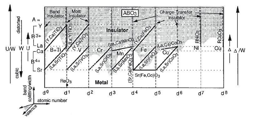
Figure 6: This diagram (due to A.Fujimori Fujimori (1992), see also Imada et al. (1998)) can be viewed as a map of the vast territory of transition- metal compounds with perovskite structure ABO₃. Varying the transition metal ion B corresponds to gradual filling of the 3d-shell. Different substitutions on the A-site can be made (A= Sr,Ca and A=La,Y are mainly considered in this diagram). This allows to change either the valence of the transition metal ion (doping), or the structural parameters in an isoelectronic manner. The shaded region corresponds to insulating compounds, while the unshaded one corresponds to metals. This illustrates the key role of the Mott phenomenon in the physics of transition-metal oxides.

A limited number of materials are poised right on the verge of this electronic instability. This is the case, for example, of V₂O₃, NiS_2-xSe_x and of quasi two-dimensional organic conductors of the $\kappa$-BEDT family. These materials are particularly interesting for the fundamental investigation of the Mott transition, since they offer the possibility of going from one phase to the other by varying some external parameter (e.g chemical composition,temperature, pressure,…). Varying external pressure is definitely a tool of choice since it allows to sweep continuously from the insulating phase to the metallic phase (and back). The phase diagrams of (V_1-x Cr_x)₂O₃ and of $\kappa$-(BEDT-TTF)₂Cu[N(CN)₂]Cl under pressure are displayed in Fig. 7.

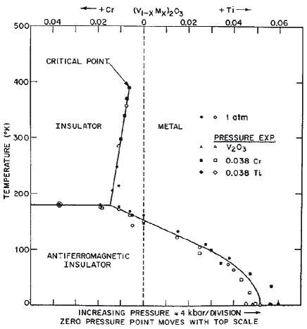
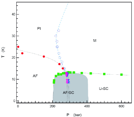
Figure 7: Left: Phase diagram of (V_1-x Cr_x)₂O₃ as a function of either Cr-concentration $x$ or pressure (afterMcWhan et al. (1973)). Increasing $x$ by $1\%$ produces similar effects than decreasing pressure by $\sim 4$kbar, for this material. Right: Phase diagram of $\kappa$-(BEDT-TTF)₂Cu[N(CN)₂]Cl as a function of pressure (after Lefebvre et al. (2000)).

There is a great similarity between the high-temperature part of the phase diagrams of these materials, despite very different energy scales. At low-pressure they are paramagnetic Mott insulators, which are turned into metals as pressure is increased. Above a critical temperature $T_{c}$ (of order $\sim 450$K for the oxide compound and $\sim 40$K for the organic one), this corresponds to a smooth crossover. In contrast, for $T<T_{c}$ a first-order transition is observed, with a discontinuity of all physical observables (e.g resistivity). The first order transition line ends in a second order critical endpoint at $(T_{c},P_{c})$. We observe that in both cases, the critical temperature is a very small fraction of the bare electronic energy scales (for V₂O₃  the half-bandwidth is of order $0.5-1$ eV, while it is of order $2000$ K for the organics).

There are also some common features between the low-temperature part of the phase diagram of these compounds, such as the fact that the paramagnetic Mott insulator orders into an antiferromagnet as temperature is lowered. However, there are also striking differences: the metallic phase has a superconducting instability for the organics, while this is not the case for V₂O₃. Also, the magnetic transition is only superficially similar : in the case of V₂O₃ , it is widely believed to be accompanied (or even triggered) by orbital orderingBao et al. (1997) (in contrast to NiS_2-xSe_xKotliar (1999b)), and as a result the transition is first-order. In general, there is a higher degree of universality associated with the vicinity of the Mott critical endpoint than in the low-temperature region, in which long-range order takes place in a material- specific manner.

Mott localization into a paramagnetic insulator implies a high spin entropy, which must therefore be quenched in some way as temperature is lowered. An obvious possibility is magnetic ordering, as in these two materials. In fact, a Mott transition between a paramagnetic Mott insulator and a metallic phase is only observed in those compounds where magnetism is sufficiently frustrated so that the transition is not preempted by magnetic ordering. This is indeed the case in both compounds discussed here: V₂O₃  has competing ferromagnetic and antiferromagnetic exchange constants, while the two-dimensional layers in the organics have a triangular structure. Another possibility is that the entropy is quenched through a Peierls instability (dimerization), in which case the Mott insulator can remain paramagnetic (this is the case, for example, of VO₂). Whether it is possible to stabilize a paramagnetic Mott insulator down to $T=0$ without breaking spin or translational symmetries is a fascinating problem, both theoretically and from the materials point of view (for a recent review on resonating valence bond phases in frustrated quantum magnets, see e.g Misguich and Lhuillier (2003) and S.Sachdev (2004)). The compound $\kappa$-(BEDT-TTF)₂Cu₂(CN)₃ may offer Shimizu et al. (2003) a realization of such a spin-liquid state (presumably through a combination of strong frustration and strong charge fluctuations Imada et al. (2003)), but this behaviour is certainly more the exception than the rule.

4.2 Dynamical mean-field theory of the Mott transition

Over the last decade, a detailed theory of the strongly correlated metallic state, and of the Mott transition itself has emerged, based on the dynamical mean-field theory (DMFT). We refer to Georges et al. (1996) for a review and an extensive list of original references Georges and Kotliar (1992); Rozenberg et al. (1992); Georges and Krauth (1992, 1993); Rozenberg et al. (1994); Laloux et al. (1994) We now review some key features of this theory.

Quasiparticle coherence scale

In the metallic state, Fermi-liquid theory applies below a low energy scale $\varepsilon_{F}^{*}$, which can be interpreted as the coherence-scale for quasiparticles (i.e long-lived quasiparticles exist only for energies and temperature smaller than $\varepsilon_{F}^{*}$). This low-energy coherence scale is given by $\varepsilon_{F}^{*}\sim ZD$ (with $D$ the half-bandwith, also equal to the Fermi energy of the non-interacting system at half-filling) where $Z$ is the quasiparticle weight. In the strongly correlated metal close to the transition, $Z\ll 1$, so that $\varepsilon_{F}^{*}$ is strongly reduced as compared to the bare Fermi energy.

Three peaks in the d.o.s: Hubbard bands and quasiparticles

In addition to low-energy quasiparticles (carrying a fraction $Z$ of the spectral weight), the one-particle spectrum of the strongly correlated metal contains high-energy excitations carrying a spectral weight $1-Z$. These are associated to the atomic-like transitions corresponding to the addition or removal of one electron on an atomic site, which broaden into Hubbard bands in the solid. As a result, the ${\bf k}$-integrated spectral function $A(\omega)=\sum_{\bf k}A({\bf k},\omega)$ (density of states d.o.s) of the strongly correlated metal is predicted Georges and Kotliar (1992) to display a three-peak structure, made of a quasiparticle band close to the Fermi energy surrounded by lower and upper Hubbard bands (Fig. 8 and inset of Fig. 14). The quasiparticle part of the d.o.s has a reduced width of order $ZD\sim\varepsilon_{F}^{*}$. The lower and upper Hubbard bands are separated by an energy scale $\Delta$.

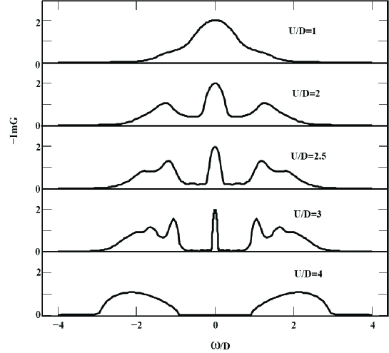
Figure 8: Local spectral function for several values of the interaction strength in DMFT. These results have been obtained using the IPT approximation, for the half-filled Hubbard model with a semi-circular d.o.s (from Ref. Georges et al. (1996)). Close to the transition, the separation of scales between the quasiparticle coherence energy ($\varepsilon_{F}^{*}$) and the distance between Hubbard bands ($\Delta\,$) is clearly seen.

The insulating phase: local moments, magnetism and frustration

At strong enough coupling (see below), the paramagnetic solution of the DMFT equations is a Mott insulator, with a gap $\Delta$ in the one-particle spectrum. This phase is characterized by unscreened local moments, associated with a Curie law for the local susceptibility $\sum_{q}\chi_{q}\propto 1/T$, and an extensive entropy. Note however that the uniform susceptiblity $\chi_{q=0}$ is finite, of order $1/J\sim U/D^{2}$. As temperature is lowered, these local moments order into an antiferromagnetic phase Jarrell (1992); Georges and Krauth (1993). The Néel temperature is however strongly dependent on frustration Georges et al. (1996) (e.g on the ratio $t^{\prime}/t$ between the next nearest-neighbour and nearest-neighbour hoppings) and can be made vanishingly small for fully frustrated models.

Separation of energy scales, spinodals and transition line

Within DMFT, a separation of energy scales holds close to the Mott transition. The mean-field solution corresponding to the paramagnetic metal at $T=0$ disappears at a critical coupling $U_{c2}$. At this point, the quasiparticle weight vanishes ($Z\propto 1-U/U_{c2}$) as in Brinkman-Rice theory On the other hand, a mean-field insulating solution is found for $U>U_{c1}$, with the Mott gap $\Delta$ opening up at this critical coupling (Mott-Hubbard transition). As a result, $\Delta$ is a finite energy scale for $U=U_{c2}$ and the quasiparticle peak in the d.o.s is well separated from the Hubbard bands in the strongly correlated metal.

These two critical couplings extend at finite temperature into two spinodal lines $U_{c1}(T)$ and $U_{c2}(T)$, which delimit a region of the $(U/D,T/D)$ parameter space in which two mean-field solutions (insulating and metallic) are found (Fig. 9). Hence, within DMFT, a first-order Mott transition occurs at finite temperature even in a purely electronic model. The corresponding critical temperature $T_{c}^{el}$ is of order $T_{c}^{el}\sim\Delta E/\Delta S$, with $\Delta E$ and $\Delta S\sim\ln(2S+1)$ the energy and entropy differences between the metal and the insulator. Because the energy difference is small ($\Delta E\sim(U_{c2}-U_{c1})^{2}/D$), the critical temperature is much lower than $D$ and $U_{c}$ (by almost two orders of magnitude). Indeed, in V₂O₃ as well as in the organics, the critical temperature corresponding to the endpoint of the first-order Mott transition line is a factor of 50 to 100 smaller than the bare electronic bandwith.

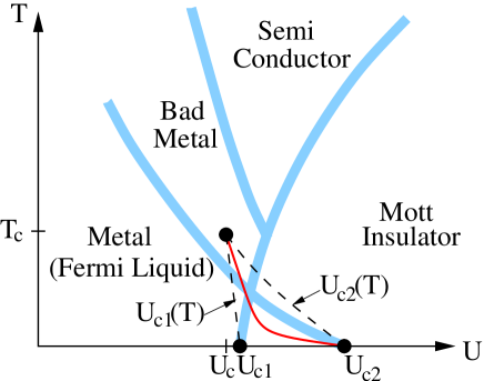
Figure 9: Paramagnetic phases of the Hubbard model within DMFT, displaying schematically the spinodal lines of the Mott insulating and metallic mean-field solutions (dashed), the first-order transition line (plain) and the critical endpoint. The shaded crossover lines separating the different transport regimes discussed in Sec.3 are also shown. The Fermi-liquid to “bad metal” crossover line corresponds to the quasiparticle coherence scale and is a continuation of the spinodal $U_{c2}(T)$ above $T_{c}$. The crossover into the insulating state corresponds to the continuation of the $U_{c1}$ spinodal. Magnetic phases are not displayed and depend on the degree of frustration. Figure from Refs. Florens (2003) and Georges et al. (2003).

4.3 Physical properties of the correlated metallic state: DMFT confronts experiments

4.3.1 Three peaks: evidence from photoemission

In Fig. 10, we reproduce the early photoemission spectra of some $d^{1}$ transition metal oxides, from the pioneering work of Fujimori and coworkers Fujimori et al. (1992). This work established experimentally, more than ten years ago, the existence of well-formed (lower) Hubbard bands in correlated metals, in addition to low-energy quasiparticles.

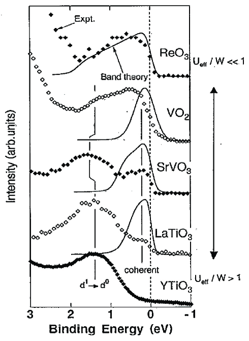
Figure 10: Photoemission spectra of several $d^{1}$ transition metal oxides, reproduced from Ref. Fujimori et al. (1992). The effects of correlations increases from ReO₃ (a weakly correlated metal) to YTiO₃ (a Mott insulator). The plain lines are the d.o.s obtained from band structure calculations. A lower Hubbard band around $-1.5$ eV is clearly visible in the most correlated materials, both in the metallic and insulating case.

This experimental study and the theoretical prediction of a 3-peak structure from DMFT Georges and Kotliar (1992) came independently around the same time. However, back in 1992, the existence of a narrow quasiparticle peak in $A(\omega)$ resembling the DMFT results was, to say the least, not obvious from these early data. Further studies Inoue et al. (1995) on Ca_1-xSr_xVO₃ therefore aimed at studying the dependence of low-energy quasiparticle spectral features upon the degree of correlations. One of the main difficulty raised by these photoemission results is that the weight $Z$ of the low-energy quasiparticle peak estimated from these early data is quite small (particularly for CaVO₃), while specific heat measurements do not reveal a dramatic mass enhancement. This triggered some discussion Inoue et al. (1995); Rozenberg et al. (1996); Imada et al. (1998) about the possibility of a strong $k$-dependence of the self-energy. A decisive insight into this question came from further experimental developments by Maiti and coworkers Maiti et al. (2001); Maiti (1997) in which it was demonstrated that the photoemission spectra are actually quite sensitive to the photon energy. Studies at different photon energies allowed these authors to extract the estimated spectra corresponding to the bulk and the surface of the material. Surface and bulk spectra were found to be very different indeed: the surface of CaVO₃ being apparently insulating-like while the bulk spectrum did show a much more pronounced quasiparticle peak. Very recently, high resolution, high-photon energy photoemission studies Sekiyama et al. (2002, 2003) clarified considerably this issue. The high photon-energy spectrum reproduced on Fig. 11 displays a clear quasiparticle d.o.s at low-energy (with a weight in good agreement with $m/m^{\star}$ and a height comparable to the LDA d.o.s), as well as a lower Hubbard band carrying the rest of the spectral weight. Moreover, recent calculations Nekrasov et al. (2002); Pavarini et al. (2003); Sekiyama et al. (2003) combining electronic structure methods and DMFT (see next section) compare favorably to the experimental spectra, on a quantitative level.

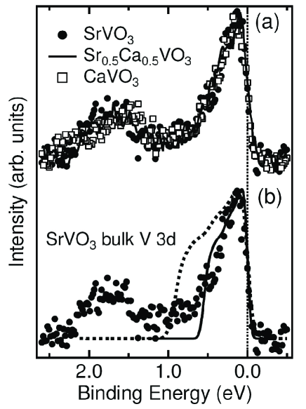
Figure 11: (a) Bulk V $3d$ spectral functions of SrVO₃ (closed circles), Sr_0.5Ca_0.5VO₃ (solid line) and CaVO₃ (open squares). (b) Comparison of the experimentally obtained bulk V $3d$ spectral function of SrVO₃ (closed circles) to the V $3d$ partial density of states for SrVO₃ (dashed curve) obtained from the band-structure calculation, which has been broadened by the experimental resolution of 140 meV. The solid curve shows the same V $3d$ partial density of states but the energy is scaled down by a factor of 0.6. Figure and caption from Ref. Sekiyama et al. (2002) (see also Sekiyama et al. (2003)).

In the case of NiS_2-xSe${}_{x}\,$, angular resolved photoemission have revealed a clear quasiparticle peak, with strong spectral weight redistributions as a function of temperature Matsuura et al. (1998). For the metallic phase of V₂O₃ , high photon energy photoemission proved to be an essential tool in the recent experimental finding of the quasiparticle peak (Fig. 12) by Mo et al. Mo et al. (2003).

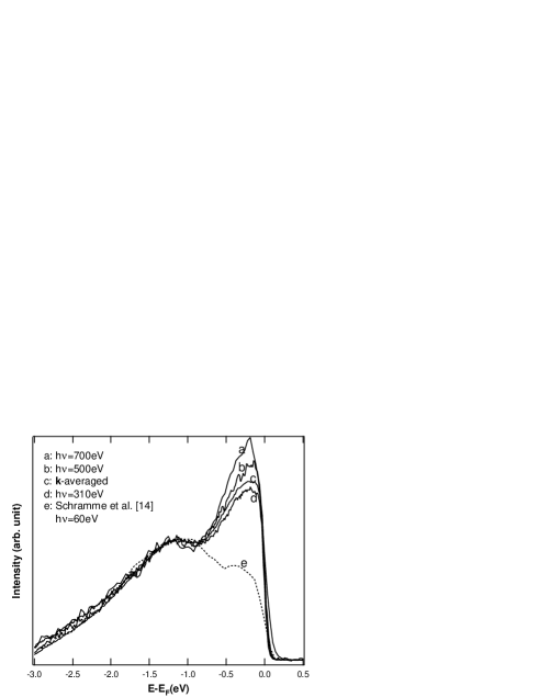
Figure 12: Photoemission spectra of V₂O₃ , for various photon energies, from Ref. Mo et al. (2003). The highest photon energy spectrum, corresponding to the greatest bulk sensitivity, reveals a prominent quasiparticle peak.

4.3.2 Spectral weight transfers

The quasiparticle peak in the d.o.s is characterized by an extreme sensitivity to changes of temperature, as shown in the inset of Fig. 14. Its height is strongly reduced as $T$ is increased, and the peak disappears altogether as $T$ reaches $\varepsilon_{F}^{*}$, leaving a pseudogap at the Fermi energy. Indeed, above $\varepsilon_{F}^{*}$, long-lived coherent quasiparticles no longer exist. The corresponding spectral weight is redistributed over a very large range of energies, of order $U$ (hence much larger than temperature itself). This is reminiscent of Kondo systems Liu et al. (1992), and indeed DMFT establishes a formal and physical connection Georges and Kotliar (1992) between a metal close to the Mott transition and the Kondo problem. The local moment present at short time-scales is screened through a self-consistent Kondo process involving the low-energy part of the (single- component) electronic fluid itself.

These spectral weight transfers and redistributions are a distinctive feature of strongly correlated systems. As already mentioned, they have been observed in the photoemission spectra of NiS_2-xSe_x . They are also commonly observed in optical spectroscopy of correlated materials, as shown on Fig. 13 for metallic V₂O₃  Rozenberg et al. (1995) and the $\kappa$-BEDT organics Eldridge et al. (1991). DMFT calculations give a good description of the optical spectral weight transfers for these materials, at least on a qualitative level Rozenberg et al. (1995); Merino and McKenzie (2000).

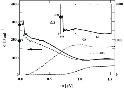
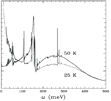
Figure 13: Left: Optical conductivity of metallic $V_{2}O_{3}$ Rozenberg et al. (1995) at $T=170K$ (thick line) and $T=300K$ (thin line)). The inset contains the difference of the two spectra $\Delta\sigma(\omega)=\sigma_{170K}(\omega)-\sigma_{300K}(\omega)$. Diamonds indicate the measured dc conductivity $\sigma_{dc}$. Dotted lines are for the insulating compounds $V_{2-y}O_{3}$ with $y=.013$ at $10K$ (upper) and $y=0$ at $70K$ (lower). Right: Optical conductivity of $\kappa$-(BEDT-TTF)₂Cu[N(CN)₂]Br at ambiant pressure Eldridge et al. (1991), for $T=25$K and $T=50$K. For both materials, transfer of spectral weight from high energies to the Drude peak is clearly visible as temperature is lowered.

4.3.3 Transport regimes and crossovers

The disappearance of coherent quasiparticles, and associated spectral weight transfers, results in three distinct transport regimes Rozenberg et al. (1995); Majumdar and Krishnamurthy (1995); Merino and McKenzie (2000); Limelette et al. (2003a); Georges et al. (2003) for a correlated metal close to the Mott transition, within DMFT (Figs. 9 and 14):

• In the Fermi-liquid regime $T\ll\varepsilon_{F}^{*}$, the resistivity obeys a $T^{2}$ law with an enhanced prefactor: $\rho=\rho_{M}\,(T/\varepsilon_{F}^{*})^{2}$. In this expression, $\rho_{M}$ is the Mott-Ioffe-Regel resistivity $\rho_{M}\propto ha/e^{2}$ corresponding to a mean-free path of the order of a single lattice spacing in a Drude picture.

• For $T\sim\varepsilon_{F}^{*}$, an “incoherent” (or “bad”) metal regime is entered. The quasiparticle lifetime shortens dramatically, and the quasiparticle peak is strongly suppressed (but still present). In this regime, the resistivity is metallic-like (i.e increases with $T$) but reaches values considerably larger than the Mott “limit” $\rho_{M}$. A Drude description is no longer applicable in this regime.

• Finally, for $\varepsilon_{F}^{*}\ll T\ll\Delta$, quasiparticles are gone altogether and the d.o.s displays a pseudogap associated with the scale $\Delta$ and filled with thermal excitations. This yields an insulating-like regime of transport, with the resistivity decreasing upon heating ($d\rho/dT<0$). At very low temperature, the resistivity follows an activated behaviour, but deviations from a pure activation law are observed at higher temperature (these two regimes are depicted as the “insulating” and “semi-conducting” ones on Fig. 9).

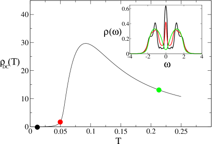
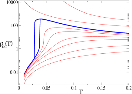
Figure 14: Left: Resistivity in the metallic phase close to the Mott transition ($U=2.4D$), as a function of temperature, calculated within DMFT using the IPT approximation. For three selected temperatures, corresponding to the three regimes discussed in the text, the corresponding spectral density is displayed in the inset. Right: IPT results for the resistivity for values of $U$ in the metallic regime (lower curves), the coexistence region (bold curve) and the insulating regime (upper two curves). From Ref. Florens (2003); Georges et al. (2003).

These three regimes, and the overall temperature dependence of the resistivity obtained within DMFT are illustrated by Fig. 14. A distinctive feature is the resistivity maximum, which occurs close to the Mott transition. This behaviour is indeed observed experimentally in both Cr-doped V₂O₃ and the organics. In the latter case, the transport data obtained recently in the Orsay group are depicted on Fig. 15, and compared to DMFT model calculations Limelette et al. (2003a); Georges et al. (2003).

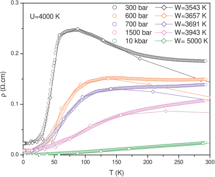
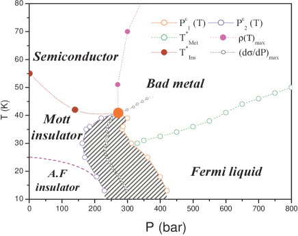
Figure 15: Left: Temperature-dependence of the resistivity at different pressures, for $\kappa$-(BEDT-TTF)₂Cu[N(CN)₂]Cl. The data (circles) are compared to a DMFT-NRG calculation (diamonds), with a pressure dependence of the bandwidth as indicated. The measured residual resistivity $\rho_{0}$ has been added to the theoretical curves. Right: Transport regimes and crossovers for this compound. Figures reproduced from Limelette et al. Limelette et al. (2003a).

Within DMFT, the conductivity can be simply obtained from a calculation of the one-particle self-energy since vertex corrections are absent Khurana (1990); Georges et al. (1996). However, a precise determination of both the real and imaginary part of the real-frequency self-energy is required. This is a challenge for most “impurity solvers”. In practice, early calculationsMajumdar and Krishnamurthy (1995); Rozenberg et al. (1995); Merino and McKenzie (2000) used the iterated perturbation theory (IPT) approximationGeorges and Kotliar (1992). The results displayed in Fig. 14 have been obtained with this technique, and the overall shape of the resistivity curves are qualitatively reasonable. However, the IPT approximation does a poor job on the quasiparticle lifetime in the low-temperature regime, as shown on Fig. 16. Indeed, we expect on general grounds that, close to the transition, $D\,\mbox{Im}\Sigma$ becomes a scaling function Moeller et al. (1995) of $\omega/\varepsilon_{F}^{*}$ and $T/\varepsilon_{F}^{*}$, so that for $T\ll\varepsilon_{F}^{*}$ it behaves as: $\mbox{Im}\Sigma(\omega=0)\propto D(T/\varepsilon_{F}^{*})^{2}\propto T^{2}/(Z^{2}D)$ which leads to an enhancement of the $T^{2}$ coefficient of the resistivity by $1/Z^{2}$ as mentioned above. The IPT approximation does not capture this enhancement and yields the incorrect result $\mbox{Im}\Sigma_{IPT}(\omega=0)\propto U^{2}T^{2}/D^{3}$, as illustrated For this reason, the numerical renormalization group (NRG) has been used recently Limelette et al. (2003a); Georges et al. (2003) in order to perform accurate transport calculations within DMFT. This method is very appropriate in this context, since it is highly accurate at low energies and yields real-frequency dataBulla et al. (2001). DMFT-NRG calculations compare favorably to transport data on organics, as shown on Fig. 15.

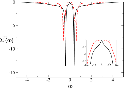
Figure 16: Comparison between the IPT (dashed lines) and NRG methods (plain lines), reproduced from Ref. Georges et al. (2003). The low-frequency behaviour of the inverse lifetime $\mbox{Im}\Sigma$ clearly displays a critically enhanced curvature, which is not reproduced by IPT.

The crossovers described here in electrical transport also have consequences for thermal transport. The thermopower, in particular, displays a saturation in the incoherent metal regime Pálsson and Kotliar (1998); Merino and McKenzie (2000). This is presumably relevant for the cobalt- based thermoelectric oxides such as Na_xCoO₂  . Finally, let me emphasize that an interesting experimental investigation of the correlations between transport crossovers (both ab-plane and c-axis) and the loss of quasiparticle coherence observed in photoemission has been performed by Valla et al.  Valla et al. (2002) for several layered materials. This study raises intriguing questions in connection with DMFT, and particularly its ${\bf k}$-dependent extensions.

4.4 Critical behaviour: a liquid-gas transition

Progress has been made recently in identifying the critical behaviour at the Mott critical endpoint, both from a theoretical and experimental standpoint. It was been pointed early on by Castellani et al.Castellani et al. (1979) (see also Jayaraman et al. (1970)) that an analogy exists with the liquid-gas transition in a classical fluid. This is based on a qualitative picture illustrated on Fig. 17. The Mott insulating phase has few double occupancies (or holes) and corresponds to a low-density “gas”, while the metallic phase corresponds to a high-density “liquid” with many double-occupancies and holes (so that the electrons can be itinerant).

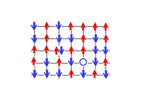
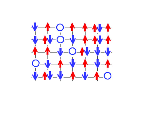
Figure 17: Cartoon of a typical real-space configuration of electrons in the Mott insulator (left) and metallic (right) phase. The insulator has few double-occupancies or holes, and corresponds to a gas of these excitations. Fluctuating local moments exist in this phase. The metal has many double-occupancies and holes, corresponding to a dense “liquid”. Electrons are itinerant in the metallic phase, and the local moments are quenched. Within DMFT this quenching is akin to a (self-consistent) local Kondo effect.

Recently, this analogy has been given firm theoretical foundations within the framework of a Landau theory Kotliar (1999a); Kotliar et al. (2000); Rozenberg et al. (1999) derived from DMFT by Kotliar and coworkers. In this framework, a scalar order parameter $\phi$ is associated with the low-energy electronic degrees of freedom which build up the quasiparticle resonance in the strongly correlated metallic phase close to the transition. This order parameter couples to the singular part of the double occupancy (hence providing a connection to the qualitative picture above), as well as to other observables such as the Drude weight or the dc-conductivity. Because of the scalar nature of the order parameter, the transition falls in the Ising universality class. In Table 1, the correspondence between the Ising model quantities, and the physical observables of the liquid-gas transition and of the Mott metal-insulator transition is summarized.

Hubbard model	Mott MIT	Liquid-gas	Ising model
$D-D_{c}$	$p-p_{c}$	$p-p_{c}$	Field $h$
			(w/ some admixture of $r$)
			Distance to
$T-T_{c}$	$T-T_{c}$	$T-T_{c}$	critical point $r$
			(w/ some admixture of $h$)
Low-$\omega$	Low-$\omega$	$v_{g}-v_{L}$	Order parameter
spectral weight	spectral weight		(scalar field $\phi$)

Table 3: Liquid-gas description of the Mott critical endpoint. The associated Landau free-energy density reads $r\phi^{2}+u\phi^{4}-h\phi$ (a possible $\phi^{3}$ can be eliminated by an appropriate change of variables and a shift of $\phi$).

In Fig. 18, the dc-conductivity obtained from DMFT in the half-filled Hubbard model (using IPT) is plotted as a function of the half-bandwith $D$, for several different temperatures. The curves qualitatively resemble those of the Ising model order parameter as a function of magnetic field (in fact, $D-D_{c}$ is a linear combination of the field $h$ and of the mass term $r$ in the Ising model field theory). Close to the critical point, scaling implies that the whole data set can be mapped onto a universal form of the equation of state:

$$\langle\phi\rangle\,=\,h^{1/\delta}\,f_{\pm}\left(h/|r|^{\gamma\delta/(\delta-1)}\right)$$ (111)

In this expression, $\gamma$ and $\delta$ are critical exponents associated with the order parameter and susceptibility, respectively: $\langle\phi\rangle\sim h^{1/\delta}$ at $T=T_{c}$ and $\chi=d\langle\phi\rangle/dh\sim|T-T_{c}|^{-\gamma}$. $f_{\pm}$ are universal scaling functions associated with $T>T_{c}$ (resp. $T<T_{c}$). A quantitative study of the critical behaviour of the double occupancy within DMFT was made in Ref. Kotliar et al. (2000), with the expected mean-field values of the exponents $\gamma=1,\delta=3$.

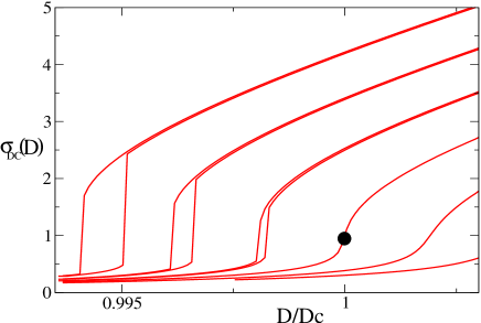
Figure 18: IPT calculation of the dc-conductivity as a function of the half-bandwith for the half-filled Hubbard model within DMFT, for several different temperatures. Increasing $D$ drives the system more metallic. The curve at $T=T_{c}$ displays a singularity (vertical slope: dot), analogous to the non-linear dependence of the order parameter upon the magnetic field at a second-order magnetic transition. Hysteretic behaviour is found for $T<T_{c}$.

Precise experimental studies of the critical behaviour at the Mott critical endpoint have been performed very recently, using a variable pressure technique, for Cr-doped V₂O₃  by Limelette et al. Limelette et al. (2003b) (Fig. 19) and also for the $\kappa$-BEDT organic compounds by Kagawa et al. Kagawa et al. (2003). These studies provide the first experimental demonstration of the liquid-gas critical behaviour associated with the Mott critical endpoint, including a a full scaling Limelette et al. (2003b) onto the universal equation of state (111).

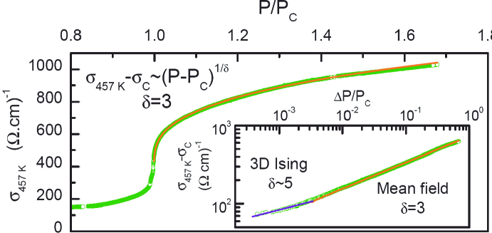
Figure 19: Conductivity of Cr-doped V₂O₃ , at the critical endpoint $T=T_{c}$, measured as a function of pressure $P/P_{c}$ (Limelette et al.  Limelette et al. (2003b)). A characteristic sigmoidal form is found, which is well fitted by $\sigma-\sigma_{c}\sim|P-P_{c}|^{1/\delta}$ (plain line). Inset: log-log scale. See Ref. Limelette et al. (2003b) for a full experimental study of the critical behaviour, including scaling onto the universal equation of state.

4.5 Coupling to lattice degrees of freedom

Lattice degrees of freedom do play a role at the Mott transition in real materials, e.g the lattice spacing changes discontinuously through the first-order transition line in (V_1-x Cr_x)₂O₃, as displayed in Fig. 20. In the metallic phase, the d-electrons participate in the cohesion of the solid, hence leading to a smaller lattice spacing than in the insulating phase.

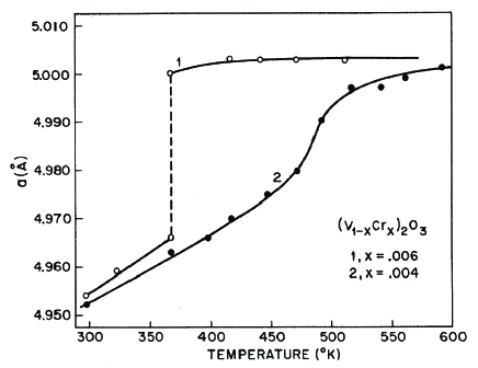
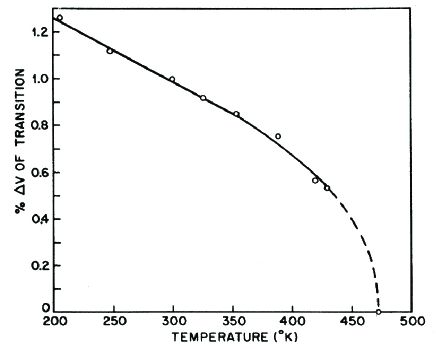
Figure 20: Left: Change of the lattice constant as a function of temperature for two samples of (V_1-xCr_x)₂O₃  with different Cr-concentrations. The discontinuous change in the lattice constant through the first-order transition transition line is clearly seen for $x=.006$, while the sample with $x=.004$ is slightly to the right of the critical point. Right: Percentage volume change of the unit-cell volume close to the critical line, reflecting the critical behaviour of the order parameter. Reproduced from Ref. Jayaraman et al. (1970)

Both the electronic degrees of freedom and the ionic positions must be retained in order to describe these effects. In Ref. Majumdar and Krishnamurthy (1994) (see also Cyrot and Lacour-Gayet (1972)), such a model was treated in the simplest approximation where all phonon excitations are neglected. The free energy then reads:

$$F=\frac{1}{2}\,B_{0}\,\frac{(v-v_{0})^{2}}{v_{0}}+F_{el}\left[D(v)\right]$$ (112)

In this expression, $v$ is the unit-cell volume, $B_{0}$ is a reference elastic modulus and the electronic part of the free-energy $F_{el}$ depends on $v$ through the volume-dependence of the bandwith. In such a model, the critical endpoint is reached when the electronic response function:

$$\chi=-\frac{\partial^{2}F_{el}}{\partial D^{2}}$$ (113)

is large enough (but not infinite), and hence the critical temperature $T_{c}$ of the compressible model is larger than $T_{c}^{el}$ (at which $\chi$ diverges in the Hubbard model). The compressibility $\kappa=\left(v\partial^{2}F/\partial v^{2}\right)^{-1}$ diverges at $T_{c}$. This implies an anomalous lowering of the sound-velocity at the transition Merino and McKenzie (2000); Hassan et al. (2004), an effect that has been experimentally observed in the $\kappa$-BEDT compounds recently Fournier et al. (2003), as shown on Fig. 21.

We emphasize that, within DMFT, an unambiguous answer is given to the “chicken and egg” question: is the first-order Mott transition driven by electronic or lattice degrees of freedom ? Within DMFT, the transition is described as an electronic one, with lattice degrees of freedom following up. In fact, it is aremarkable finding of DMFT that a purely electronic model can display a first-order Mott transition and a finite-T critical endpoint (associated with a diverging $\chi$), provided that magnetism is frustrated enough so that ordering does not preempt the transition. Whether this also holds for the finite-dimensional Hubbard model beyond DMFT is to a large extent an open question (see Onoda and Imada (2003) for indications supporting this conclusion in the 2D case).

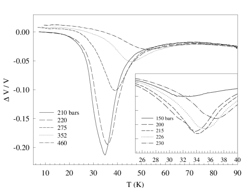
Figure 21: Relative change in the sound velocity of $\kappa$-(BEDT-TTF)₂Cu[N(CN)₂]Cl as a function of temperature, at various pressures. The velocity variation is relative to the value at 90 K. Inset: position and amplitude of the anomaly below 230 bars. (Figure and caption from Ref. Fournier et al. (2003)).

4.6 The frontier: ${\bf k}$-dependent coherence scale, cold and hot spots

A key question, still largely open, in our theoretical understanding of the Mott transition is the role of spatial correlations (inadequately treated by DMFT). This is essential in materials like cuprates, in which short-range spatial correlations play a key role (in particular magnetic correlations due to superexchange, leading to a strong tendency towards the formation of singlet bonds, as well as pair correlations). In the regime where the quasiparticle coherence scale $\varepsilon_{F}^{*}$ is small as compared to the (effective strength of the) superexchange $J$, the DMFT picture is certainly deeply modified. There is compelling experimental evidence that the quasiparticle coherence scale then has a strong variation as the momentum ${\bf k}$ is varied along the Fermi surface, leading to the formation of “cold spots” and “hot regions”. Such effects have been found in recent studies using cluster extensions of the DMFT framework (Parcollet et al. (2003), see also Biermann et al. (2001); Giamarchi et al. (2004)).

5 Electronic structure and Dynamical Mean-Field Theory

The possibility of using DMFT in combination with electronic structure calculation methods, in order to overcome some of the limitations of DFT-LDA for strongly correlated materials, was pointed out early on Georges et al. (1996). In the last few years, very exciting developments have taken place, in which theorists from the electronic structure and many-body communities joined forces and achieved concrete implementations of DMFT within electronic structure calculations. The first papers Anisimov et al. (1997a); Lichtenstein and Katsnelson (1998) implementing this combination appeared in 1997-1998, and the field has been extremely active since then. For reviews of the early developments in this field, see Refs. Held et al. (2001a, b); Kotliar and Savrasov (2001); Lichtenstein et al. (2002). For on-line material presented at recent workshops, see Refs. kit (2002a, b); ict (2003)

5.1 Limitations of DFT-LDA for strongly correlated systems

In Sec. 3.2, I briefly presented the basic principles of density functional theory (DFT). In practice, the local density approximation (LDA) to the exchange-correlation energy, and its extensions (such as the generalised gradient approximation) have been remarkably successful at describing ground-state properties of many solids from first principles. This is also the state of the art method for band structure calculations, with the additional assumption that Kohn-Sham eigenvalues can be interpreted as single-particle excitations. For strongly correlated materials however, DFT-LDA has severe limitations, which we now briefly review.

Issues about ground-state properties

Ground-state properties, such as equilibrium unit-cell volume, are not accurately predicted from LDA (or even GGA) for the most strongly correlated materials. This is particularly true of materials in which some electrons are very localized, such as the 4f electrons of rare-earth elements at ambiant or low pressure (Sec. 1.3.3). If these orbitals are treated as valence orbitals, the LDA leads to a much too itinerant character, and therefore overestimates the contribution of these orbitals to the cohesive energy of the solids, hence leading to a too small unit-cell volume. If instead the f-orbitals are treated as core states, the equilibrium volume is then overestimated (albeit closer to experimental value, in the case of rare earth), since binding is underestimated. Phenomena such as the volume-collapse transitions, associated with the partial delocalization of the f-electrons, (and associated structural changes) under pressure McMahan et al. (1998) are simply out of reach of standard methods. At high pressures however, the f-electrons recover itinerant character and DFT-LDA(GGA) does better, as expected. In some particular cases, the electrons are just on the verge of the itinerant/localized behaviour. In such cases, standard electronic structure methods perform very poorly. A spectacular example is the $\delta$-phase of metallic plutonium in which the unit-cell volume is underestimated (compared to the experimental value) by as much as $35\%$ by standard electronic structure methods (Fig. 24) ! All these examples illustrate the need of a method which is able to handle intermediate situations between fully localized and fully itinerant electrons. I emphasize that this issue may depend crucially on energy scales, with localized character most pronounced at high-energy (short time) scales, and itinerant quasiparticles forming at low-energy (long time scales).

Excitation spectra

Even though the Kohn-Sham eigenvalues and wavefunctions are, strictly speaking, auxiliary quantities in the DFT formalism used to represent the local density, they are commonly interpreted as energy bands in electronic structure calculations. This is very successful in many solids, but does fail badly in strongly correlated ones. The most spectacular difficulty is that Mott insulators are found to have metallic Kohn-Sham spectra. This is documented, e.g by Fig. 23, in which the LDA density of states of two Mott insulators, LaTiO₃  and YTiO₃  are shown. I emphasize that, in both compounds (as well as in many other Mott insulators), the Mott insulating gap has nothing to do with the magnetic ordering in the ground-state. Even though magnetic long-range order is found at low-enough temperatures in both materials (below $T_{N}\simeq 140$ K in LaTiO₃  and $T_{\,C}\simeq 30$ K in YTiO₃ ), the insulating behaviour and Mott gap ($\simeq 1\,\mbox{eV}\,$ for YTiO₃ ) are maintained well above the ordering temperature. In other cases (such as VO₂ ), the insulating phase is a paramagnet and the LDA spectrum is again metallic.

In strongly correlated metals, e.g close to Mott insulators, the LDA bandstructure is also in disagreement with experimental observations. The two main discrepancies are the following. (i) LDA single-particle bands are generally too broad. Correlation effects lead to band-narrowing, corresponding to a (Brinkman-Rice) enhancement of the effective masses of quasiparticles. This becomes dramatic in f-electron materials, where the large effective mass is due to the Kondo effect, a many-body process which is beyond the reach of single-particle theories. (ii) The spectral weight $Z$ associated with quasiparticles is reduced by correlations, and the corresponding missing spectral weight $1-Z$ is found in intermediate or high-energy incoherent excitations. In correlated metals, as well as in Mott insulators, lower and upper Hubbard bands are observed, which are absent in the LDA density of states (e.g for SrVO₃  and CaVO₃  in Fig. 11 and Fig 23).

Related correlation effects are observed also for pure transition metals, such as nickel, in which the LDA spectrum is unable to account for: the $\sim-6\,\mbox{eV}\,$ photoemission satellite, and for the correct values of the occupied bandwidth and exchange splitting between the majority and minority band in the ferromagnetic ground-state.

5.2 Marrying DMFT and DFT-LDA

In this section, I briefly describe the (happy) marriage of electronic structure methods and dynamical mean-field theory. I first give a simple practical formulation in terms of a realistic many-body hamiltonian, and keep for the next section the construction of energy functionals.

The first issue to be discussed is the choice of the basis set for the valence electrons. Since DMFT emphasizes local correlations, we need a localised basis set, i.e basis functions which are centered on the atomic positions ${\bf R}$ in the crystal lattice. Up to now, most implementations have used basis sets based on linear muffin-tin orbitals Andersen (1975); Skriver (1984) (LMTOs) $\chi_{L{\bf R}}({\bf r})=\chi_{L}({\bf r}-{\bf R})$ (in which $L=\{l,m\}$ stands for the angular momentum quantum number of the valence electrons). These basis sets offer the advantage to carry over the physical intuition of atomic orbitals from the isolated atoms to the solid. In the words of their creator, O.K. Andersen, LMTO- based electronic structure methods are “intelligible” because they are based on a minimal and flexible basis set of short-range orbitals Andersen et al. (2000). There are several possible choices of basis even within the LMTO method. Basically, a compromise has to be made between the degree of localisation and the orthogonality of the basis set. The most localised basis set (the so-called “screened” or $\alpha$-basis) is not orthogonal and will therefore involve an overlap matrix $O_{LL^{\prime}}=\langle\chi_{L}|\chi_{L^{\prime}}\rangle$. Since DMFT neglects non-local correlations, they may be the best one to choose. However, a non-orthogonal basis set may not be simple to implement, for technical reasons, when using some impurity solvers (e.g QMC). Orthogonal LMTOs basis sets are somewhat more extended.

Another possibility is to use basis sets made of Wannier functions. This has been little explored yet in combination with DMFT. Wannier functions can in fact be constructed starting from the LMTO formalism by using the “downfolding” procedure (the so-called third-generation LMTO Andersen et al. (2000, 2000)). Recently, DMFT has been implemented within a downfolded (NMTO) Wannier basis, and successfully applied to transition metal oxides with non-cubic structures. Other routes to Wannier functions (such as the Marzari-Vanderbilt construction of maximally localised Wannier functions Marzari and Vanderbilt (1997)) might be worth pursuing. Given a basis set, the electron creation operator at a point ${\bf r}$ in the solid can be decomposed as:

$$\psi^{\dagger}({\bf r})=\sum_{{\bf R},L}\chi^{*}_{L{\bf R}}({\bf r})\,c_{L{\bf R}}^{\dagger}$$ (114)

The decomposition of the full Green’s function in the solid: $G({\bf r},{\bf r}^{\prime},\tau-\tau^{\prime})\equiv-\langle T\psi({\bf r},\tau)\psi^{\dagger}({\bf r}^{\prime},\tau^{\prime})\rangle$ (as well as of any other one-particle quantity) thus reads:

$$G({\bf r},{\bf r}^{\prime},i\omega)=\sum_{{\bf R}{\bf R}^{\prime}}\sum_{LL^{\prime}}\chi_{L{\bf R}}({\bf r})G_{LL^{\prime}}({\bf R}-{\bf R}^{\prime},i\omega)\chi_{L^{\prime}{\bf R}^{\prime}}({\bf r}^{\prime})^{*}$$ (115)

The simplest combination of DMFT and electronic structure methods uses a starting point which is similar to that of the LDA$+$U approach Anisimov et al. (1991); Anisimov et al. (1997b). Namely, one first separates the valence electrons into two groups: those for which standard electronic structure methods are sufficient on one hand (e.g $l=s,p$ in an oxide or $l=s,p,d$ in rare-earth compounds), and on the other hand the subset of orbitals which will feel strong correlations (e.g $l=d$ or $l=f$). This separation refers, of course, to the specific choice of basis set which has been made. In the following, I denote the orbitals with $l$ in the correlated subset by the index $a\equiv\{m,\sigma\}$ (and $b,\cdots$). Let us then consider the one-particle hamiltonian:

$$H_{KS}=\sum_{\lambda}\epsilon^{KS}_{\lambda}|\lambda\rangle\langle\lambda|=\sum_{{\bf k}L}h^{KS}_{LL^{\prime}}({\bf k})c^{\dagger}_{{\bf k}L}c_{{\bf k}L^{\prime}}$$ (116)

obtained from solving the Kohn-Sham equations for the material under consideration. The Kohn-Sham potential we have in mind is, in the simplest implementation, the one obtained within a standard DFT-LDA (or GGA) electronic structure calculation of the local density. In a more sophisticated implementation, one may also correct the local density by correlation effects and use the associated Kohn-Sham potential (i.e modify the self-consistency cycle over the local density in comparison to standard LDA, see below). A many-body hamiltonian is then constructed as follows:

$$H=H_{KS}-H_{DC}+H_{U}$$ (117)

In this expression, $H_{U}$ are many-body terms acting in the subset of correlated orbitals only. They correspond to matrix elements of the Coulomb interaction, and will in general involve arbitrary 2-particle terms $U_{abcd}c^{\dagger}_{a}c^{\dagger}_{b}c_{d}c_{c}$. In practice however, one often makes a further simplification and keep only density-density interactions (for technical reasons, this is always done when using QMC as a solver). To simplify notations, we shall limit ourselves here to this case, and use:

$$H_{U}=\frac{1}{2}\sum_{\bf R}\sum_{ab\sigma}U_{ab}\,\hat{n}_{{\bf R}a}\hat{n}_{{\bf R}b}$$ (118)

with:

$$U_{mm^{\prime}}^{\uparrow\downarrow}=U_{mm^{\prime}}\,\,\,,\,\,\,U_{m\neq\,m^{\prime}}^{\uparrow\uparrow}=U_{m\neq\,m^{\prime}}^{\downarrow\downarrow}=U_{mm^{\prime}}-J_{mm^{\prime}}$$ (119)

In this expression, $J_{mm^{\prime}}$ is the Hund’s coupling. For a more detailed discussion of the choice of the matrix of interaction parameters, see e.g Ref. Anisimov et al. (1997b).

The “double-counting” term $H_{DC}$ needs to be introduced, since the contribution of interactions between the correlated orbitals to the total energy is already partially included in the exchange-correlation potential. Unfortunately, it is not possible to derive this term explicitly, since the energy within DFT is a functional of the total electron density, which combines all orbitals in a non-linear manner. In practice, the most commonly used form of the double-counting term is (for other choices, see e.g Lichtenstein et al. (2001)):

$$H_{DC}=\sum_{{\bf R}\sigma ab}V^{DC}_{ab\sigma}c^{\dagger}_{a\sigma}c_{b\sigma}$$

$$V^{DC}_{ab\sigma}=\delta_{ab}\left[U(N-\frac{1}{2})-J(N^{\sigma}-\frac{1}{2})\right]$$ (120)

The many-body hamiltonian (117) is then soved using the DMFT approximation. This means that a local self-energy matrix is assumed, which acts in the subset of correlated orbitals only:

$$\Sigma^{{\bf R}{\bf R}^{\prime}}_{LL^{\prime}}(i\omega)\,=\,\delta_{{\bf R},{\bf R}^{\prime}}\,\left(\begin{array}[]{cc}0&0\\ 0&\Sigma_{ab}(i\omega)\\ \end{array}\right)$$ (121)

In the DMFT framework, the local Green’s function in the correlated subset:

$$G_{ab}(\tau-\tau^{\prime})\equiv-\langle Tc^{\dagger}_{a}(\tau)c_{b}(\tau^{\prime})\rangle$$ (122)

is represented as the Green’s function of the multi-orbital impurity model:

$$S=-\int^{\beta}_{0}d\tau\int^{\beta}_{0}d\tau^{\prime}\,\sum_{ab}c^{\dagger}_{a}(\tau)[{\cal G}_{0}^{-1}]_{ab}(\tau-\tau^{\prime})c_{b}(\tau^{\prime})+\frac{1}{2}\sum_{ab}\,U_{ab}\,\int^{\beta}_{0}d\tau\,n_{a}(\tau)n_{b}(\tau)$$ (123)

The Weiss function (or alternatively the dynamical mean-field, or effective hybridisation function $\Delta_{ab}=(i\omega_{n}+\mu)\delta_{ab}-[{\cal G}_{0}^{-1}]_{ab}$) is determined, as before, from the self-consistency condition requesting that the on-site Green’s function in the solid coincides with the impurity model Green’s function. The components of the Green’s function of the solid in the chosen basis set read:

$$[G^{-1}]_{LL^{\prime}}({\bf k},i\omega_{n})=(i\omega_{n}+\mu)\delta_{LL^{\prime}}-h^{KS}_{LL^{\prime}}+V^{DC}_{LL^{\prime}}-\Sigma_{LL^{\prime}}(i\omega_{n})$$ (124)

In this expression, the self-energy matrix $\Sigma_{LL^{\prime}}$ is constructed by using the components of the impurity self-energy $\Sigma_{ab}\equiv[{\cal G}_{0}^{-1}]_{ab}-[G_{imp}^{-1}]_{ab}$ into (121). The self-consistency condition relating implicitly ${\cal G}_{0}$ and $G_{imp}$ finally reads:

$$G(i\omega_{n})_{ab}\,=\,\sum_{{\bf k}}\,\left[(i\omega_{n}+\mu)\delta_{LL^{\prime}}-h^{KS}_{LL^{\prime}}+V^{DC}_{LL^{\prime}}-\Sigma_{LL^{\prime}}(i\omega_{n})\right]^{-1}_{ab}$$ (125)

Note that this involves a matrix inversion at each ${\bf k}$-point, as well as a ${\bf k}$-summation over the Brillouin zone (which does not, in general, reduces to an integration over the band density of states, in contrast to the single-band case). Also let us emphasize that, even though the self-energy matrix has only components in the subspace of correlated orbitals, the components of the Green’s function corresponding to all valence orbitals ($s,p,d,\cdots$) are modified due to the matrix inversion. Correlation effects encoded in the self-energy affect the local electronic density, which can be calculated from the full Green’s function as:

$$\rho({\bf r})\,=\,\sum_{\bf k}\,\chi_{L{\bf k}}({\bf r})\,G_{LL^{\prime}}({\bf k},\tau=0^{-})\,\chi_{L^{\prime}{\bf k}}^{*}({\bf r})$$ (126)

In a complete implementation, self-consistency over the local density should also be reached Savrasov et al. (2001); Kotliar and Savrasov (2001). The general structure of the combination of DMFT with electronic structure calculations, as well as the iterative procedure used in practice to solve the DMFT equations, is summarised on Fig. 22.

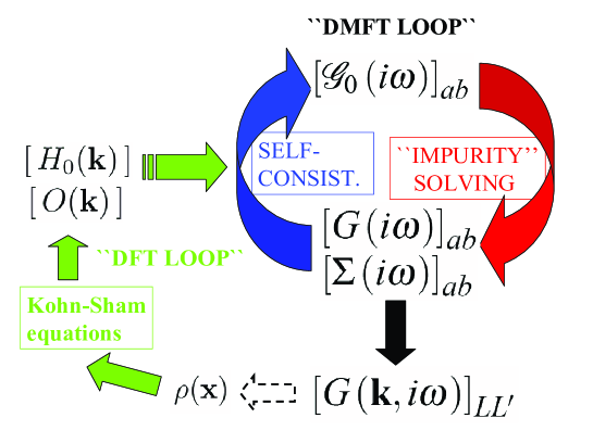
Figure 22: DMFT combined with electronic structure calculations. Starting from a local electronic density $\rho({\bf r})$, the associated Kohn-Sham potential is calculated and the Kohn-Sham equations are solved. The Kohn-Sham hamiltonian $H^{KS}_{LL^{\prime}}({\bf k})$ is expressed in a localised basis set (e.g LMTOs). A double-counting term is substracted to obtain the one-electron hamiltonian $H_{0}\equiv H^{KS}-H^{DC}$. The local self-energy matrix for the subset of correlated orbitals is obtained through the iteration of the DMFT loop: a multi-orbital impurity model for the correlated subset is solved (red arrow), containing as an input the dynamical mean-field (or Weiss field ${\cal G}_{0}$). The self-energy $\Sigma_{ab}$ is combined with $H_{0}$ into the self-consistency condition Eq. (125) in order to update the Weiss field (blue arrow). At the end of the DMFT loop, the components of the full, ${\bf k}$-dependent, Green’s function in the local basis set can be calculated and thus also an updated local density $\rho({\bf r})$. This is used (dashed arrow) as a new starting density for the Kohn-Sham calculation until a converged local density is also reached . Alternatively, in a simplified implementation of this full scheme, the DFT-LDA calculation can be converged first and the corresponding $H_{0}$ injected into the DMFT loop without attempting to update $\rho({\bf r})$.

5.3 An application to $d^{1}$ oxides

On Fig. 23, I show the spectral functions recently obtained in Ref. Pavarini et al. (2003) for SrVO₃ , CaVO₃ , LaTiO₃  and YTiO₃ . These oxides have the same formal valence of the d-shell ($d^{1}$). The single electron sits in the $t_{2g}$ multiplet, and the (empty) $e_{g}$ doublet is well separated in energy. They have a perovskite structure with perfect cubic symmetry for the first one (Fig. 2) and increasing degree of structural distortion for the three others (corresponding mainly to the GdFeO₃-like tilting of oxygen octahedra). These calculations were performed in a downfolded (NMTO) basis set, including the off-diagonal components of the self-energy matrix. The latter are important for the compounds with the largest structural distortions. For comparison, the LDA density of states are shown on the same plot. For an independent DMFT calculation of the Ca/SrVO₃ compounds, see Ref. Nekrasov et al. (2002); Sekiyama et al. (2003) and Ref. Anisimov et al. (1997a); Nekrasov et al. (2000) for early calculations of the doped system La_1-xSr_xTiO₃ . The spectra in Fig. 23 have features which should be familiar to the reader at this point, namely:

• SrVO₃  and CaVO₃  are correlated metals with lower ($\sim-1.5$ eV) and upper ($\sim 2.5$ eV) Hubbard bands, as well as a relatively moderate narrowing of the quasiparticle bandwith. The calculated spectra compare favorably to the recent photoemission experiments of Fig. 11 (see Sekiyama et al. (2003) for a comparison).

• LaTiO₃  and YTiO₃  are Mott insulators, with quite different values of the Mott gap ($\sim 0.3$ eV and $\sim 1$ eV, respectively) as observed experimentally. It was emphasized in Pavarini et al. (2003) that the main reason for this difference is that the orbital degeneracy of the $t_{2g}$ multiplet is lifted to a greater degree in YTiO₃  than in LaTiO₃  due to the larger structural distortion. Indeed, reducing orbital degeneracy is known to increase the effect of correlations (for comparable interaction strength) Gunnarsson et al. (1997); Koch et al. (1999); Florens et al. (2002); Manini et al. (2002). It was also found in Ref. Pavarini et al. (2003) that both compounds develop a very pronounced orbital polarization, of a quite different nature in each compound (see Mochizuki and Imada (2003) for a discussion of orbital ordering in these materials and Cwik et al. (2003) for a recent experimental investigation).

This example, as well as several other recent studies, demonstrate that the embedding of DMFT within electronic structure calculations yields a powerful quantitative tool for understanding the rich interplay between correlation effects and material-specific aspects.

Figure 23: LDA+DMFT spectral densities of the transition-metal oxides discussed in the text, from Ref. Pavarini et al. (2003). The (QMC) calculations were made at $T=770$K. For comparison, the LDA d.o.s are also displayed (thin lines).

5.4 Functionals and total- energy calculations

In order to discuss total energy calculations in the LDA$+$DMFT framework, it is best to use a formulation of this scheme in terms of a (free-) energy functional. Kotliar and Savrasov Kotliar and Savrasov (2001); Savrasov and Kotliar (2003) have introduced for this purpose a (“spectral-density-”) functional of both the total local electron density $\rho({\bf r})$ and the on-site Green’s function in the correlated subset: $G_{ab}^{{\bf R}{\bf R}}$ (denoted $G_{ab}$ for simplicity in the following). Let us emphasize that these quantities are independent, since $G_{ab}$ is restricted to local components and to a subset of orbitals so that $\rho({\bf r})$ cannot be reconstructed from it. The functional is constructed by introducing (see Section. 3) source terms $\lambda({\bf r})=v_{KS}({\bf r})-v_{c}({\bf r})$ and $\Delta\Sigma_{ab}(i\omega_{n})$ coupling to the operators $\psi^{\dagger}({\bf r})\psi({\bf r})$ and to $\sum_{{\bf R}}\chi^{*}_{a}({\bf r}-{\bf R})\psi({\bf r},\tau)\psi^{\dagger}({\bf r}^{\prime},\tau^{\prime})\chi_{b}({\bf r}^{\prime}-{\bf R})=c_{a{\bf R}}(\tau)c^{\dagger}_{b{\bf R}}(\tau^{\prime})$, respectively. Furthermore, the Luttinger-Ward part of the functional is approximated by that of the on-site local many-body hamiltonian $H_{U}-H_{DC}$ introduced above. This yields:

$$\Omega[\rho({\bf r}),G_{ab};v_{KS}({\bf r}),\Delta\Sigma\,_{ab}]_{LDA+DMFT}\,=$$

$$-\mbox{tr}\,\ln[i\omega_{n}+\mu+\frac{1}{2}\nabla^{2}-v_{KS}({\bf r})-\chi^{*}.\Delta\Sigma\,.\chi]-\int d{\bf r}\,(v_{KS}-v_{c})\rho({\bf r})-\mbox{tr}\,[G.\Delta\Sigma\,]+$$

$$+\frac{1}{2}\int d{\bf r}\,d{\bf r}^{\prime}\rho({\bf r})U({\bf r}-{\bf r}^{\prime})\rho({\bf r}^{\prime})+E_{xc}[\rho({\bf r})]+\sum_{\bf R}\left(\Phi_{imp}[G^{{\bf R}{\bf R}}_{ab}]-\Phi_{DC}[G^{{\bf R}{\bf R}}_{ab}]\right)$$

In this expression, $\chi^{*}.\Delta\Sigma\,.\chi$ denotes the “upfolding” of the local quantity $\Delta\Sigma\,$ to the whole solid: $\chi^{*}.\Delta\Sigma\,.\chi=\sum_{\bf R}\sum_{ab}\chi^{*}_{a}({\bf r}-{\bf R})\Sigma_{ab}(i\omega_{n})\chi_{b}({\bf r}^{\prime}-{\bf R})$. Variations of this functional with respect to the sources $\delta\Omega/\delta\,v_{KS}=0$ and $\delta\Omega/\delta\Sigma_{ab}=0$ yield the standard expression of the local density and local Green’s function in terms of the full Green’s function in the solid:

$$\rho({\bf r})=\langle{\bf r}|\hat{G}|{\bf r}\rangle\,\,\,,\,\,\,G_{ab}(i\omega_{n})=\langle\chi_{a{\bf R}}|\hat{G}|\chi_{b{\bf R}}\rangle$$ (127)

with:

$$\hat{G}=\left[i\omega_{n}+\mu+\frac{1}{2}\nabla^{2}-v_{KS}({\bf r})-\chi^{*}.\Delta\Sigma\,.\chi\right]^{-1}$$ (128)

or, in the local basis set (see (124)):

$$\hat{G}=\sum_{{\bf k},LL^{\prime}}|\chi_{L{\bf k}}\rangle\left[(i\omega_{n}+\mu).1-\hat{h}^{KS}({\bf k})-\Delta\hat{\Sigma}(i\omega_{n})\right]^{-1}_{LL^{\prime}}\langle\chi_{L^{\prime}{\bf k}}|$$ (129)

From these relations, the Legendre multiplier functions $v_{KS}$ and $\Delta\Sigma\,$ could be eliminated in terms of $\rho$ and $G_{ab}$, so that a functional of the local observables only is obtained:

$$\Gamma_{LDA+DMFT}[\rho,G_{ab}]=\Omega_{LDA+DMFT}\left[\rho({\bf r}),G_{ab};\lambda[\rho,G],\Delta\Sigma\,[\rho,G]\right]$$ (130)

Extremalisation of this functional with respect to $\rho$ ($\delta\Gamma/\delta\rho=0$) and $G_{ab}$ ($\delta\Gamma/\delta\,G_{ab}=0$) yields the expression of the Kohn-Sham potential and self-energy correction at self-consistency:

$$v_{KS}({\bf r})=v_{c}({\bf r})+\int d{\bf r}^{\prime}U({\bf r}-{\bf r}^{\prime})\rho({\bf r}^{\prime})+\frac{\delta E_{xc}}{\delta\rho({\bf r})}$$ (131)

$$\Delta\Sigma\,_{ab}=\frac{\delta\Phi_{imp}}{\delta\,G_{ab}}-\frac{\delta\Phi_{DC}}{\delta\,G_{ab}}\equiv\Sigma^{imp}_{ab}-V^{DC}_{ab}$$ (132)

Hence, one recovers from this functional the defining equations of the LDA$+$DMFT combined scheme, including self-consistency over the local density (127). Using (66) and (61), one notes that the free-energy can be written as:

$$\Omega_{LDA+DMFT}=\Omega_{DFT}+\mbox{tr}\,\ln\,G_{KS}({\bf k},i\omega_{n})^{-1}-\mbox{tr}\,\ln\,G({\bf k},i\omega_{n})^{-1}-\mbox{tr}\,[G_{imp}\Sigma^{imp}]+\sum_{\bf R}\Phi_{imp}+$$

$$+\mbox{tr}\,[G_{imp}V^{DC}]-\sum_{\bf R}\Phi_{DC}$$ (133)

In this expression, $\Omega_{DFT}$ is the usual density-functional theory expression (66), while $G_{KS}$ is the Green’s function corresponding to the Kohn-Sham hamiltonian, i.e without the self-energy correction:

$$G_{KS}^{-1}\equiv i\omega_{n}+\mu-\hat{h}_{KS}({\bf k})$$ (134)

A careful examination of the zero-temperature limit of (133) leads to the following expression of the total energy Amadon et al. (2003):

$$E_{LDA+DMFT}\,=\,E_{DFT}-\sum^{\prime}_{\lambda}\varepsilon^{KS}_{\lambda}+\langle H_{KS}\rangle+\langle H_{U}\rangle-E_{DC}$$ (135)

$$=E_{DFT}+\sum_{{\bf k},LL^{\prime}}h^{KS}_{LL^{\prime}}[\langle c^{\dagger}_{L{\bf k}}c_{L^{\prime}{\bf k}}\rangle_{DMFT}-\langle c^{\dagger}_{L{\bf k}}c_{L^{\prime}{\bf k}}\rangle_{KS}]+\langle H_{U}\rangle-E_{DC}$$ (136)

The first term, $E_{DFT}$ is the energy found within DFT(LDA), using of course the local density obtained at the end of the LDA$+$DMFT convergence cycle, namely:

$$E_{DFT}=\sum^{\prime}_{\lambda}\varepsilon^{KS}_{\lambda}+\int d{\bf r}[v_{c}({\bf r})-v_{KS}({\bf r})]\rho({\bf r})+\frac{1}{2}\int d{\bf r}d{\bf r}^{\prime}\rho({\bf r})u({\bf r}-{\bf r}^{\prime})\rho({\bf r}^{\prime})+E_{xc}[\rho]$$ (137)

Hence the total energy within LDA$+$DMFT is made of several terms. Importantly, it does not simply reduce to the expectation value $\langle H\rangle$ of the many-body hamiltonian (117) introduced in the previous section. Furthermore, $\langle H_{KS}\rangle=\mbox{tr}\,[H_{KS}\hat{G}]$ must be evaluated with the full Green’s function including the self-energy correction. Therefore, this quantity does not coincide with the sum of the (occupied) Kohn-Sham eigenvalues $\sum^{\prime}_{\lambda}\epsilon^{KS}_{\lambda}=\mbox{tr}\,H_{KS}G_{KS}$. Eq. (135) expresses that the latter has to be removed from $E_{DFT}$, in order to correctly take into account the change of energy coming from the Kohn-Sham orbitals. This change can also be written $\langle H_{KS}\rangle_{DMFT}-\langle H_{KS}\rangle_{KS}=\mbox{tr}\,[(G-G_{KS})H_{KS}]$. This is used in the second expression for the energy, which emphasizes the modification of the density matrix $\langle\,c^{\dagger}_{L{\bf k}}c_{L^{\prime}{\bf k}}\rangle$ by correlations. Finally, the double-counting correction to the energy is the zero-temperature limit of $-\langle H_{DC}\rangle+\mbox{tr}\,[G\Sigma^{DC}]-\Phi_{DC}$. The simplest form of double-counting correction (neglecting $J$ for simplicity) corresponds to: $\Phi_{DC}[G_{ab}]=U\,N(N-1)/2$ with $N=\sum_{a}n_{a}=\sum_{a}\mbox{tr}\,G_{aa}$. Hence $V^{DC}_{ab}=\delta\Phi_{DC}/\delta\,G_{ab}=U(N-1/2)n_{a}\delta_{ab}$, and $\langle H_{DC}\rangle=\mbox{tr}\,[G\Sigma^{DC}]=UN(N-1/2)$ so that, finally: $E_{DC}=U\,N(N-1)/2$.

Another formula for the total energy within LDA+DMFT has been used by Held et al. in their investigation of the volume collapse transition of Cerium Held et al. (2001); McMahan et al. (2003).

Total energy calculations within LDA$+$DMFT, with full self-consistency on the local density have been performed by Savrasov, Kotliar and Abrahams Savrasov et al. (2001); Kotliar and Savrasov (2001); Savrasov and Kotliar (2003) for metallic plutonium with fcc structure, corresponding to the $\delta$-phase. The results are reproduced in Fig. 24, in which the total energy is plotted as a function of the unit-cell volume (normalised by the experimental value), for different values of the parameter $U$. It is seen that the GGA calculation underestimates the volume by more than $30\%$. As $U$ increases, the minimum is pushed to higher volumes, and good agreement with experiments is reached for $U$ in the range $3.8-4\,\mbox{eV}\,$. Interestingly, in the presence of correlations, the energy curve develops a metastable shallow minimum at a lower volume, which can be interpreted as a manifestation of the $\alpha$-phase (which has a more complicated crystal structure however). For the corresponding spectra, see Savrasov and Kotliar (2003). In these DMFT calculations, the $\delta$-phase of plutonium is described as a paramagnetic metal, in agreement with experiments. In contrast, a static LDA$+$U treatmentSavrasov and Kotliar (2000); Bouchet et al. (2000) also corrects the equilibrium volume, but at the expense of introducing an unphysical spin polarization.

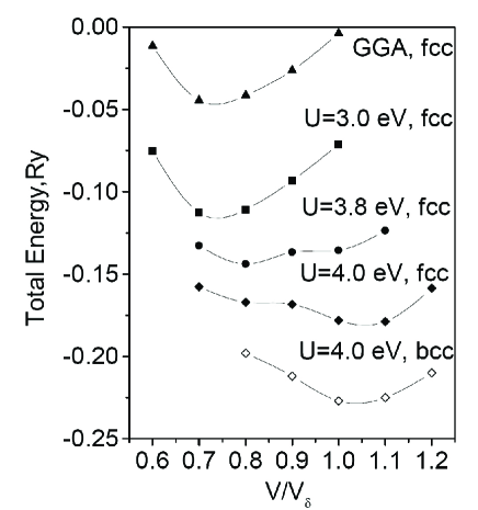
Figure 24: Total energy of fcc plutonium as a function of unit-cell volume (normalised by the experimental volume of the $\delta$-phase), reproduced from Ref. Savrasov et al. (2001); Savrasov and Kotliar (2003). The upper curve is the GGA result. Other curves are from LDA+DMFT with different values of $U$. The lower curve is for the bcc structure.

5.5 A life without U: towards ab-initio DMFT

The combination of DMFT with electronic structure methods described in the previous section introduces a matrix $U$ of local interaction parameters acting in the subset of correlated orbitals, as in the LDA$+$U scheme. Some of these parameters can be determined from constrained LDA calculations, or instead they can be viewed as adjustable. Furthermore, introducing these interactions implies the need for a “double-counting” correction in order to remove the contribution to the total energy already taken into account in the (orbital-independent) exchange correlation potential. As such, this theory has great practical virtues. However, going beyond this framework and being able to treat the electron-electron interaction entirely from first- principles is a tempting and challenging project. Work in this direction have appeared recently Biermann et al. (2003); Kotliar and Savrasov (2001); Sun and Kotliar (2002, 2003); Biermann et al. (2004); Aryasetiawan et al. (2003, 2004).

Physically, the Hubbard interaction is associated with the screened Coulomb interaction as seen by a given atom in the solid. Screening is essential for estimating the order of magnitude of this parameter correctly. The naive view that $U$ is simply the on-site matrix element of the Coulomb potential in the local basis- set would lead to values on the scale of tens of electron-volts, while the appropriate value in the solid is a few eV’s ! This immediately points towards a key notion: that, in fact, the Hubbard $U$ is a concept which depends on the energy-scale. At high energies (say, above the plasma frequency in a metal), it has a very large value associated with the bare, unscreened, matrix element, while at low energy screening takes place and it is considerably reduced. For first-principle RPA studies of the frequency dependence of the screened local interaction, see Springer and Aryasetiawan (1998); Aryasetiawan et al. (2004).

In fact, the screened effective interaction in a solid can be related, quite generally, to the density-density correlation function. Let us start from the first-principles hamiltonian:

$$H=-\sum_{i}\frac{1}{2}\nabla^{2}_{i}+\sum_{i}v({\bf r}_{i})+\frac{1}{2}\sum_{i\neq j}u({\bf r}_{i}-{\bf r}_{j})$$

$$=-\frac{1}{2}\int d{\bf r}\psi^{\dagger}\nabla^{2}\psi+\int d{\bf r}\,v({\bf r})\hat{n}({\bf r})+{1\over 2}\int d{\bf r}d{\bf r}^{\prime}\,u({\bf r}-{\bf r}^{\prime})\,:\hat{n}({\bf r})\hat{n}({\bf r}^{\prime}):$$ (138)

in which $u({\bf r}-{\bf r}^{\prime})=e^{2}/|{\bf r}-{\bf r}^{\prime}|$ is the bare Coulomb interaction, $\hat{n}\equiv\psi^{\dagger}({\bf r})\psi({\bf r})$ and $:(\,):$ denotes normal ordering. The (connected) density-density correlation function is defined as:

$$\chi({\bf r},{\bf r}^{\prime};\tau-\tau^{\prime})=\langle T\,(\hat{n}({\bf r},\tau)-\rho({\bf r}))\,(\hat{n}({\bf r}^{\prime},\tau^{\prime})-\rho({\bf r}^{\prime})\rangle$$ (139)

with $\rho({\bf r})=\langle\hat{n}({\bf r})\rangle$ the local density. The screened effective interaction reads:

$$W({\bf r},{\bf r}^{\prime},i\omega)=u({\bf r}-{\bf r}^{\prime})-\int d{\bf r}_{1}\,d{\bf r}_{2}\,u({\bf r}-{\bf r}_{1})\chi({\bf r}_{1}-{\bf r}_{2};i\omega)u({\bf r}_{2}-{\bf r}^{\prime})$$ (140)

This can also be expressed in terms of the polarization $P\equiv-\chi.[1-u.\chi]^{-1}$ as $W=u.[1-P.u]^{-1}$ (the dot is an abbreviation for spatial convolutions). We emphasize that in this expression, $P$ is the exact polarization operator, not its RPA approximation. The screened interaction $W$ can be interpreted as the correlation function of the local scalar potential field conjugate to $\hat{n}({\bf r})$, as can be shown from a Hubbard-Stratonovich transformation.

Armed with this precise formal definition of the screened interaction in the solid (and, naturally, also of the full Green’s function $G({\bf r},{\bf r}^{\prime};\tau-\tau^{\prime})\equiv-\langle T\psi({\bf r},\tau)\psi^{\dagger}({\bf r}^{\prime},\tau^{\prime})\rangle$), we would like to adopt now a local picture in which we focus on a given atom. This is done,as before, by specifying a complete basis set of functions $\chi_{L{\bf R}}({\bf r})$ localised around the atomic positions ${\bf R}$. There is of course some arbitrariness in this choice, as already discussed. Adopting a local point of view, we focus on the matrix elements of the Green’s function and of the screened effective interaction on a given atomic site:

$$G_{ab}(i\omega)=\langle\chi_{a{\bf R}}|G|\chi_{b{\bf R}}\rangle\,\,\,,\,\,\,W_{a_{1}a_{2}a_{3}a_{4}}(i\omega)=\langle\chi_{a_{1}{\bf R}}\chi_{a_{2}{\bf R}}|W|\chi_{a_{3}{\bf R}}\chi_{a_{4}{\bf R}}\rangle$$ (141)

In this expression, the indices $a,b,\cdots$ can run over the full set of valence orbitals, or alternatively over a subset corresponding to the more strongly correlated ones. This is a matter of choice of the local quantities we decide to focus on. Following the point of view developed in the third section of these lectures, the key idea is again to introduce an exact representation of these local quantities as the solution of an atomic problem coupled to an effective bath. Because we want to represent the local components of both $G$ and $W$, this effective problem now involves two Weiss functions, both in the one-particle and two-particle sectors. This is an extended form of dynamical mean-field theory (EDMFT). The action of the local problem reads:

$$S=\int d\tau d\tau^{\prime}\left[-\sum c_{a}^{+}(\tau){\cal G}_{ab}^{-1}(\tau-\tau^{\prime})c_{b}(\tau^{\prime})+\right.$$

$$\left.+\frac{1}{2}\,\sum:c_{a_{1}}^{+}(\tau)c_{a_{2}}(\tau):\mathcal{U}_{a_{1}a_{2}a_{3}a_{4}}(\tau-\tau^{\prime}):c_{a_{3}}^{+}(\tau^{\prime})c_{a_{4}}(\tau^{\prime}):\right]$$ (142)

The local screened interaction is calculated from this effective action as: $W_{imp}={\cal U}-{\cal U}\chi_{imp}{\cal U}$ with $\chi_{imp}$ the 2-particle impurity correlation funcition. The two Weiss fields ${\cal G}$ and ${\cal U}$ are adjusted in such a way that $G_{imp}=G_{ab}$ and $W_{imp}=W_{abcd}$, the local quantities in the solid. The impurity model (142) can be viewed as an atom hybridised with an effective bath of non-interacting fermions and also coupled to a bath of fluctuating electric scalar potentials.

This construction provides an unambiguous definition of the Hubbard interactions ${\cal U}_{abcd}(i\omega)$ in the solid (as well as of the usual dynamical mean-field ${\cal G}$), assuming of course that the local components of the screened interaction $W$ and of the Green’s function $G$ are known. Frequency- dependence of ${\cal U}$ is essential in a proper definition of these Hubbard interactions, at least when a wide range of energy scale is considered. Naturally, one degree of arbitrariness remains, associated with the choice of the basis set: ${\cal U}$ will change when a different basis set is considered, keeping the same form of the effective interaction $W({\bf r},{\bf r}^{\prime};i\omega)$ in the full solid.

To proceed from these formal considerations to a practical scheme, we need to decide how $W$ and $G$ will actually be calculated, and this of course will involve approximations. Again, a free-energy functional is an excellent guidance and indeed such a functional of the full $G({\bf r},{\bf r^{\prime}};i\omega)\,$ and $W({\bf r},{\bf r^{\prime}};i\omega)\,$ has been introduced by Almbladh et al.Almbladh et al. (1999), generalizing the Baym-Kadanoff construction (see also Chitra and Kotliar (2001) for independent work). The functional reads:

$$\Gamma(G,W)=Tr\ln G-Tr[(G_{H}^{-1}-G^{-1})G]-\frac{1}{2}Tr\ln W+\frac{1}{2}Tr[(u^{-1}-W^{-1})W]+\Psi[G,W]$$ (143)

$G_{H}^{-1}=i\omega_{n}+\mu+\nabla^{2}/2-v_{H}$ corresponds to the Hartree Green’s function with $v_{H}$ being the Hartree potential. For a derivation of (143) using a Hubbard-Stratonovich transformation and a Legendre transformation with respect to both $G$ and $W$, see Chitra and Kotliar (2001). The functional $\Psi[G,W]$ is a generalization of the Luttinger-Ward functional $\Phi[G]$, whose derivative with respect to $G$ gives the self-energy. Here we have, similarly (from $\delta\Gamma/\delta\,G=\delta\Gamma/\delta\,W=0$):

$$G^{-1}=G_{H}^{-1}-\Sigma^{xc}\,\,\,,\,\,\,\Sigma^{xc}=\frac{\delta\Psi}{\delta G}\,\,\,;\,\,\,W^{-1}=u^{-1}-P\,\,\,,\,\,\,P=-2\frac{\delta\Psi}{\delta W}$$ (144)

A well established electronic structure calculation method, which offers in part an alternative to DFT-LDA, is the so-called GW approach Hedin (1965) (see Aryasetiawan and Gunnarsson (1998) for a review). This corresponds to the following approximation to the $\Psi$-functional:

$$\Psi_{GWA}\,=\,-\,\frac{1}{2}\,\int d{\bf r}d{\bf r}^{\prime}\int d\tau d\tau^{\prime}\,G({\bf r},{\bf r}^{\prime},\tau-\tau^{\prime})W({\bf r},{\bf r}^{\prime},\tau-\tau^{\prime})G({\bf r}^{\prime},{\bf r},\tau^{\prime}-\tau)$$ (145)

which yields the RPA-like approximation to the polarisation and exchange-correlation self-energy: $P=G\star\,G$ and $\Sigma^{xc}=-G\star\,W$. The GW approximation to the $\Psi$-functional is easily written in terms of the components of $G$ and $W$ in the chosen basis set:

$$\Psi_{GWA}=-\frac{1}{2}\int d\tau\sum_{L_{1}\cdots L_{2}^{\prime}}\sum_{{\bf R}{\bf R}^{\prime}}G^{{\bf R}{\bf R}^{\prime}}_{L_{1}L^{\prime}_{1}}(\tau)W^{{\bf R}{\bf R}^{\prime}}_{L_{1}L_{2}L^{\prime}_{1}L^{\prime}_{2}}(\tau)G^{{\bf R}^{\prime}{\bf R}}_{L_{2}^{\prime}L_{2}}(-\tau)$$ (146)

This can be separated into a contribution $\Psi_{GWA}^{non-loc}$ from non-local components (corresponding to the terms with ${\bf R}\neq{\bf R}^{\prime}$ in (146)) and a contribution $\Psi_{GWA}^{loc}[G^{{\bf R}{\bf R}},W^{{\bf R}{\bf R}}]$ from local components only (${\bf R}={\bf R}^{\prime}$).

The GW approximation does treat the screened Coulomb interaction from first-principles, but does not treat successfully strong correlation effects. Recently, it has been suggested to improve on the GWA for the local contributions by using the DMFT framework Biermann et al. (2003); Sun and Kotliar (2002) (see also Kotliar and Savrasov (2001); Sun and Kotliar (2003); Biermann et al. (2004); Aryasetiawan et al. (2003)). One can think of different approximations to the $\Psi$-functional in this context, depending on whether the DMFT approach is used for all the valence orbitals $L=s,p,d,\cdots$, or for a subset (corresponding to the index $a,b,...$) of correlated orbitals only. The corresponding $\Psi$-functional reads:

$$\Psi_{GW+DMFT}[G^{{\bf R}{\bf R}^{\prime}}_{L_{1}L^{\prime}_{1}},W^{{\bf R}{\bf R}^{\prime}}_{L_{1}L_{2}L^{\prime}_{1}L^{\prime}_{2}}]\,=\,\Psi_{GWA}^{non-loc}+[\Psi_{GWA}^{loc}-\Delta\Psi]+\sum_{\bf R}\Psi_{imp}[G^{{\bf R}{\bf R}}_{ab},W^{{\bf R}{\bf R}}_{abcd}]$$ (147)

In this expression, $\Psi_{imp}$ is the $\Psi$-functional corresponding to the local effective model (142), while $\Delta\Psi$ removes the components from $\Psi_{GWA}^{loc}$ which will be taken into account in $\Psi_{imp}$, namely:

$$\Delta\Psi=-\frac{1}{2}\sum_{\bf R}\int d\tau\sum_{abcd}G^{{\bf R}}_{ab}(\tau)W^{{\bf R}{\bf R}}_{abcd}(\tau)G^{{\bf R}{\bf R}}_{DC}(-\tau)$$ (148)

If all valence orbitals are included in the DMFT treatment, the second term in the r.h.s of (147) is absent altogether. If only a correlated subset is treated with DMFT, $\Delta\Psi$ can be thought of as a term preventing double-counting of interactions in the correlated subset. In this context however, in contrast to LDA$+$DMFT, the form of this double-counting correction is known explicitly.

Taking derivatives of this functional with respect to the components of $G$ and $W$, one sees that, in the GW$+$DMFT approach, the non-local components of the self-energy and of the polarization operator keep the same form as in the GWA, while the local components are replaced by the ones from the effective impurity model (possibly in the correlated subset only). The GW$+$DMFT theoretical framework is fully defined by (147) and the form of the impurity model (142). As before, an interative self-consistent process must be followed in order to obtain the self-energy and screened effective interaction, as well as the dynamical mean-field ${\cal G}$ and effective Hubbard interactions ${\cal U}$. This is described in more details in Refs. Biermann et al. (2003, 2004); Aryasetiawan et al. (2003). Concrete implementations of this scheme to electronic structure (and to model hamiltonians as well) is currently being pursued by several groups. For early results, see Biermann et al. (2003); Sun and Kotliar (2002, 2003); Biermann et al. (2004); Aryasetiawan et al. (2003, 2004).

6 Conclusion and perspectives

In these lectures notes, I have tried to give an introduction to some aspects of the physics of strong electron correlations in solids. Naturally, only a limited number of topics could be covered. The field is characterized by a fascinating diversity of material-dependent properties. It is, to a large extent, experimentally driven, and new discoveries are undoubtedly yet to come. Also, new territories outside the traditional boundaries of solid-state physics are currently being explored, such as correlation effects in nano-electronic devices or the condensed matter physics of cold atoms in optical lattices.

On the theory side, these lectures are influenced by the author’s prejudice that (i) physics on intermediate energy scale matters and may be a key to the unusual behaviour of many strongly correlated materials and that (ii) quantitative theoretical techniques are essential to the development of the field, in combination with phenomenological considerations and experimental investigations.

Dynamical mean-field theory is a method of choice for treating these intermediate energy scales. The basic principles of this approach have been reviewed in these lectures. On the formal side, analogies with classical mean-field theory and density-functional theory have been emphasized, through the construction of free-energy functionals of local observables. A distinctive aspect of DMFT is that it treats quasi-particle excitations and higher energy incoherent excitations, on equal footing. As a result, it is able to describe transfers of spectra weight between quasiparticle and incoherent features as temperature, coupling strength, or some other external parameter (doping, pressure,…) is varied. I have emphasized that the quasiparticle coherence scale plays a key role in the physics of a strongly correlated metal. Above this scale, which can be dramatically reduced by correlations, unusual (non-Drude) transport and spectroscopic properties are observed, corresponding to an incoherent metallic regime. This is the case, in particular, for metals which are close to a Mott insulating phase. I have briefly reviewed the DMFT description of these effects in these lectures, in comparison to experiments, as well as the detailed theory of the Mott transition which has been one of the early successes of this approach. I have also provided an (admittedly quite succinct) introduction to the recent combination of DMFT with electronic structure calculations. These developments have been made possible by researchers from two communities joining forces towards a common goal. It provides us with a powerful quantitative tool for investigating material-dependent aspects of strong electron correlations.

Despite these successes, some key open questions in the physics of strongly correlated electron systems remain out of reach of the simplest version of DMFT. Indeed, in materials like cuprates, short-range spatial correlations play a key role (in particular magnetic correlations due to superexchange, leading to a strong tendency towards the formation of singlet bonds, as well as pair correlations). These correlations deeply affect the nature of quasiparticles. There is compelling experimental evidence that the quasiparticle coherence scale has thus a strong variation as the momentum ${\bf k}$ is varied along the Fermi surface, leading to the formation of “cold spots” and “hot regions”. Extending the DMFT framework in order to take these effects into account may well be the most important frontier in the field.

References

- Mott (1949) Mott, N. F., Proc. Phys. Soc. A, 62, 416 (1949).
- Mott (1990) Mott, N. F., Metal-insulator transitions, Taylor and Francis, London, 1990.
- Georges et al. (1996) Georges, A., Kotliar, G., Krauth, W., and Rozenberg, M. J., Reviews of Modern Physics, 68, 13–125 (1996).
- T.Pruschke et al. (1995) T.Pruschke, M.Jarrell, and J.Freericks, Adv. Phys., 42, 187 (1995).
- Springer and Aryasetiawan (1998) Springer, M., and Aryasetiawan, F., Phys. Rev. B, 57, 4364–4368 (1998).
- Aryasetiawan et al. (2004) Aryasetiawan, F., Imada, M., Georges, A., Kotliar, G., Biermann, S., and Lichtenstein, A. I., ArXiv Condensed Matter e-prints (2004), cond-mat/0401620.
- Hubbard (1963) Hubbard, J., Proc. Roy. Soc. (London), A 276, 238 (1963).
- Hubbard (1964a) Hubbard, J., Proc. Roy. Soc. (London), A 277, 237 (1964a).
- Hubbard (1964b) Hubbard, J., Proc. Roy. Soc. (London), A281, 401 (1964b).
- Varma and Giamarchi (1991) Varma, C. M., and Giamarchi, T., Model for oxide metals and superconductors, Elsevier, 1991, les Houches Summer School.
- Imada et al. (1998) Imada, M., Fujimori, A., and Tokura, Y., Rev. Mod. Phys., 70, 1039 (1998).
- Tsuda et al. (2000) Tsuda, N., Nasu, K., Fujimori, A., and Siratori, K., Electronic Conduction in Oxides, Springer Series in Solid-State Sciences 94, Springer, Berlin, 2000, 2nd edn., ISBN 3-540-66956-6.
- Harrison (1989) Harrison, W. A., Electronic structure and the properties of solids, Dover Pub., New York, 1989.
- Friedel (1969) Friedel, J., The physics of metals, Cambridge University Press, New York, 1969, pp. 494–525.
- McMahan et al. (1998) McMahan, A. K., Huscroft, C., Scalettar, R. T., and Pollock, E. L., J. Comput.-Aided Mater. Des., 5, 131 (1998), cond-mat/9805064.
- Wills and Eriksson (2000) Wills, J., and Eriksson, O., Los Alamos Science, 26, 128 (2000).
- Anisimov and Gunnarsson (1991) Anisimov, V. I., and Gunnarsson, O., Phys. Rev. B, 43, 7570–7574 (1991).
- Maiti (1997) Maiti, K., Ph.D. thesis, IISC, Bangalore (1997).
- Fujimori and Minami (1984) Fujimori, A., and Minami, F., Phys. Rev. B, 30, 957 (1984).
- Zaanen et al. (1985) Zaanen, J., Sawatzky, G. A., and Allen, J. W., Phys. Rev. Lett., 55, 418 (1985).
- Kotliar and Savrasov (2003) Kotliar, G., and Savrasov, S. Y., International Journal of Modern Physics B, 17, 5101–5109 (2003).
- Coleman (2002) Coleman, P., Lectures on the Physics of Highly Correlated Electron Systems, American Institute of Physics, New York, 2002, vol. VI, chap. Local moment physics in heavy electron systems, pp. 79–160, cond-mat/0206003.
- Hewson (1993) Hewson, A. C., The Kondo problem to heavy fermions, Cambridge University Press, 1993.
- Burdin et al. (2000) Burdin, S., Georges, A., and Grempel, D. R., Physical Review Letters, 85, 1048–1051 (2000).
- Metzner and Vollhardt (1989) Metzner, W., and Vollhardt, D., Phys. Rev. Lett., 62, 324 (1989).
- Georges and Kotliar (1992) Georges, A., and Kotliar, G., Phys. Rev. B, 45, 6479–6483 (1992).
- Jarrell (1992) Jarrell, M., Phys. Rev. Lett., 69, 168–171 (1992).
- Georges (2002) Georges, A., “Exact functionals, effective actions and dynamical mean-field theories: some remarks.,” in Strongly Correlated Fermions and Bosons in Low-Dimensional Disordered Systems, edited by I. et al., Kluwer Acad., 2002, vol. 72 of NATO Science Series-II: Mathematics, Physics and Chemistry.
- Rozenberg et al. (1992) Rozenberg, M. J., Zhang, X. Y., and Kotliar, G., Phys. Rev. Lett., 69, 1236 (1992).
- Georges and Krauth (1992) Georges, A., and Krauth, W., Phys. Rev. Lett., 69, 1240–1243 (1992).
- Hirsch and Fye (1986) Hirsch, J. E., and Fye, R. M., Phys. Rev. Lett., 25, 2521 (1986).
- Bulla et al. (2001) Bulla, R., Costi, T. A., and Vollhardt, D., Phys. Rev. B, 64, 45103 (2001).
- Kajueter and Kotliar (1996) Kajueter, H., and Kotliar, G., Phys. Rev. Lett., 77 (1996).
- Florens and Georges (2002) Florens, S., and Georges, A., Phys. Rev. B, 66, 165111–+ (2002).
- Oudovenko et al. (2004) Oudovenko, V., Haule, K., Savrasov, S. Y., Villani, D., and Kotliar, G., ArXiv Condensed Matter e-prints (2004), cond-mat/0401539.
- Schiller and Ingersent (1996) Schiller, A., and Ingersent, K., Phys. Rev. Lett., 75, 113 (1996).
- Hettler et al. (1998) Hettler, M. H., Tahvildar-Zadeh, A. N., Jarrell, M., Pruschke, T., and Krishnamurthy, H. R., Phys. Rev. B, 58, 7475– (1998).
- Kotliar et al. (2001) Kotliar, G., Savrasov, S., Palsson, G., and Biroli, G., Phys. Rev. Lett., 87, 186401 (2001).
- Biermann et al. (2001) Biermann, S., Georges, A., Lichtenstein, A., and Giamarchi, T., Physical Review Letters, 87, 276405 (2001).
- Biroli et al. (2003) Biroli, G., Parcollet, O., and Kotliar, G. (2003), cond-mat/0307587.
- Onoda and Imada (2003) Onoda, S., and Imada, M. (2003), cond-mat/0304580.
- Si and Smith (1996) Si, Q., and Smith, J. L., Phys. Rev. Lett., 77, 3391 (1996).
- Kajueter (1996) Kajueter, H., PhD thesis, Rutgers University (1996).
- Sengupta and Georges (1995) Sengupta, A. M., and Georges, A., Phys. Rev. B, 52, 10295–10302 (1995).
- Smith and Si (2000) Smith, J. L., and Si, Q., Phys. Rev. B, 61, 5184 (2000).
- Fukuda et al. (1996) Fukuda, R., Kotani, T., and Yokojima, S., Prog. Theor. Phys. Suppl., 121, 1 (1996).
- Chitra and Kotliar (2001) Chitra, R., and Kotliar, G., Phys. Rev. B, 63, 115110 (2001).
- Plefka (1982) Plefka, T., J. Phys. A, 15, 1971 (1982).
- Georges and Yedidia (1991) Georges, A., and Yedidia, J. S., Journal of Physics A Mathematical General, 24, 2173–2192 (1991).
- Polchinsky (1984) Polchinsky, J., Nucl. Phys. B, 231, 269 (1984).
- Schehr and Doussal (2003) Schehr, G., and Doussal, P. L., preprint cond-mat/030486 (2003).
- Chauve and Doussal (2001) Chauve, P., and Doussal, P. L., Phys. Rev. E, 64, 051102 (2001).
- Thouless et al. (1977) Thouless, D., Anderson, P., and Palmer, R., Phil. Mag., 35, 593 (1977).
- Mermin (1965) Mermin, N., Phys. Rev., 137, A1441 (1965).
- Hohenberg and Kohn (1964) Hohenberg, P., and Kohn, W., Phys. Rev., 136, B864 (1964).
- Kohn and Sham (1965) Kohn, W., and Sham, L., Phys. Rev., 140, A1133 (1965).
- Fukuda et al. (1994) Fukuda, R., Kotani, T., Suzuki, Y., and Yokojima, S., Prog. Theor. Phys., 92, 833 (1994).
- Valiev and Fernando (1997) Valiev, M., and Fernando, G., Phys. Lett. A, 227, 265 (1997).
- Argaman and Makov (2000) Argaman, N., and Makov, G., Am. J. Phys., 68, 69 (2000), preprint physics/9806013.
- Dreizler and Gross (1990) Dreizler, R., and Gross, E., Density Functional Theory, Springer-Verlag, 1990.
- Jones and Gunnarsson (1989) Jones, R., and Gunnarsson, O., Rev. Mod. Phys., 61, 689 (1989).
- Chayes and Chayes (1984) Chayes, J., and Chayes, L., J. Stat. Phys., 36, 471 (1984).
- Chayes et al. (1985) Chayes, J., Chayes, L., and Ruskai, M. B., J. Stat. Phys., 38, 497 (1985).
- Harris (1984) Harris, J., Phys. Rev. A, 29, 1648 (1984).
- Khodel et al. (1994) Khodel, V. A., Shaginyan, V. R., and Khodel, V. V., Physics Reports, 249, 1 (1994).
- Amusia et al. (2003) Amusia, M. Y., Msezane, A. Z., and Shaginyan, V. R. (2003), arXiv cond-mat/0312162.
- Chitra and Kotliar (2000) Chitra, R., and Kotliar, G., Phys. Rev. B, 62, 12715 (2000).
- Kotliar (1999a) Kotliar, G., Eur. J. Phys. B, 27, 11 (1999a).
- Johansson (1974) Johansson, B., Phil. Mag., 30, 469 (1974).
- Skriver et al. (1978) Skriver, H. L., Andersen, O. K., and Johansson, B., Physical Review Letters, 41, 42–45 (1978).
- Skriver et al. (1980) Skriver, H. L., Andersen, O. K., and Johansson, B., Physical Review Letters, 44, 1230–1233 (1980).
- Savrasov and Kotliar (2000) Savrasov, S. Y., and Kotliar, G., Physical Review Letters, 84, 3670–3673 (2000).
- Savrasov et al. (2001) Savrasov, S. Y., Kotliar, G., and Abrahams, E., Nature, 410, 793 (2001).
- Fujimori (1992) Fujimori, A., J. Phys. Chem. Solids, 53, 1595 (1992).
- McWhan et al. (1973) McWhan, D. B., Menth, A., Remeika, J. P., Brinckman, W. F., and Rice, T. M., Phys. Rev. B, 7, 1920 (1973).
- Lefebvre et al. (2000) Lefebvre, S., Wzietek, P., Brown, S., Bourbonnais, C., Jérome, D., Mèziére, C., Fourmigué, M., and Batail, P., Phys. Rev. Lett., 85, 5420 (2000).
- Bao et al. (1997) Bao, W., Broholm, C., Aeppli, G., Dai, P., Honig, J. M., and Metcalf, P., Phys. Rev. Lett., 78, 507 (1997).
- Kotliar (1999b) Kotliar, G., Physica B, 259-261, 711 (1999b).
- Misguich and Lhuillier (2003) Misguich, G., and Lhuillier, C., Frustrated spin systems, World Scientific, Singapore, 2003, chap. Two-dimensional quantum antiferromagnets, cond-mat/0310405.
- S.Sachdev (2004) S.Sachdev (2004), cond-mat/0401041.
- Shimizu et al. (2003) Shimizu, Y., Miyagawa, K., Kanoda, K., Maesato, M., and Saito, G. (2003), cond-mat/0307483.
- Imada et al. (2003) Imada, M., Mizusaki, T., and Watanabe, S., cond-mat/0307022 (2003).
- Georges and Krauth (1993) Georges, A., and Krauth, W., Phys. Rev. B, 48, 7167–7182 (1993).
- Rozenberg et al. (1994) Rozenberg, M. J., Kotliar, G., and Zhang, X. Y., Phys. Rev. B, 49, 10181 (1994).
- Laloux et al. (1994) Laloux, L., Georges, A., and Krauth, W., Phys. Rev. B, 50, 3092–3102 (1994).
- Florens (2003) Florens, S., Cohérence et localisation dans les systèmes d’électrons fortement corrélés, Ph.D. thesis, Université Paris 6 and Ecole Normale Supérieure, Paris (2003).
- Georges et al. (2003) Georges, A., Florens, S., and Costi, T. A., ArXiv Condensed Matter e-prints (2003), cond-mat/0311520.
- Fujimori et al. (1992) Fujimori, A., Hase, I., Namatame, H., Fujishima, Y., Tokura, Y., Eisaki, H., Uchida, S., Takegahara, K., and de Groot, F. M. F., Phys. Rev. Lett., 69, 1796 (1992).
- Inoue et al. (1995) Inoue, I. H., Hase, I., Aiura, Y., Fujimori, A., Haruyama, Y., Maruyama, T., and Nishihara, Y., Physical Review Letters, 74, 2539–2542 (1995).
- Rozenberg et al. (1996) Rozenberg, M. J., Inoue, I. H., Makino, H., Iga, F., and Nishihara, Y., Physical Review Letters, 76, 4781–4784 (1996).
- Maiti et al. (2001) Maiti, K., Sarma, D. D., Rozenberg, M., Inoue, I., Makino, H., Goto, O., Pedio, M., and Cimino, R., Europhys. Lett., 55, 246 (2001).
- Sekiyama et al. (2002) Sekiyama, A., Fujiwara, H., Imada, S., Eisaki, H., Uchida, S. I., Takegahara, K., Harima, H., Saitoh, Y., and Suga, S., ArXiv Condensed Matter e-prints (2002), cond-mat/0206471.
- Sekiyama et al. (2003) Sekiyama, A., Fujiwara, H., Imada, S., Suga, S., Eisaki, H., Uchida, S. I., Takegahara, K., Harima, H., Saitoh, Y., Nekrasov, I. A., Keller, G., Kondakov, D. E., Kozhevnikov, A. V., Pruschke, T., Held, K., Vollhardt, D., and Anisimov, V. I., ArXiv Condensed Matter e-prints (2003), cond-mat/0312429.
- Nekrasov et al. (2002) Nekrasov, I., Keller, G., Kondakov, D., Kozhevnikov, A., Pruschke, T., Held, K., Vollhardt, D., and Anisimov, V. (2002), cond-mat/0211508.
- Pavarini et al. (2003) Pavarini, E., Biermann, S., Poteryaev, A., Lichtenstein, A. I., Georges, A., and Andersen, O. K., ArXiv Condensed Matter e-prints (2003), cond-mat/0309102.
- Matsuura et al. (1998) Matsuura, A. Y., Watanabe, H., Kim, C., Doniach, S., Shen, Z. X., Thio, T., and Bennett, J. W., Phys. Rev. B, 58, 3690 (1998).
- Mo et al. (2003) Mo, S. K., Denlinger, J. D., Kim, H. D., Park, J. H., Allen, J. W., Sekiyama, A., Yamasaki, A., Kadono, K., Suga, S., Saitoh, Y., Muro, T., Metcalf, P., Keller, G., Held, K., Eyert, V., Anisimov, V. I., and Vollhardt, D., Phys. Rev. Lett., 90, 186403 (2003).
- Liu et al. (1992) Liu, L., Allen, J., Gunnarsson, O., Christansen, N., and Andersen, O., Phys. Rev. B, 45, 8934 (1992).
- Rozenberg et al. (1995) Rozenberg, M. J., Kotliar, G., Kajueter, H., Thomas, G. A., Rapkine, D. H., Honig, J. M., and Metcalf, P., Phys. Rev. Lett., 75, 105 (1995).
- Eldridge et al. (1991) Eldridge, J., Kornelsen, K., Wang, H., Williams, J., Crouch, A., and Watkins, D., Sol. State. Comm., 79, 583 (1991).
- Merino and McKenzie (2000) Merino, J., and McKenzie, R. H., Phys. Rev. B, 61, 7996 (2000).
- Majumdar and Krishnamurthy (1995) Majumdar, P., and Krishnamurthy, H., Phys. Rev. B, 52 (1995).
- Limelette et al. (2003a) Limelette, P., Wzietek, P., Florens, S., Georges, A., Costi, T. A., Pasquier, C., Jérome, D., Mézière, C., and Batail, P., Physical Review Letters, 91, 016401 (2003a).
- Khurana (1990) Khurana, A., Phys. Rev. Lett., 64, 1990 (1990).
- Moeller et al. (1995) Moeller, G., Si, Q., Kotliar, G., Rozenberg, M., and Fisher, D. S., Phys. Rev. Lett., 74, 2082 (1995).
- Pálsson and Kotliar (1998) Pálsson, G., and Kotliar, G., Phys. Rev. Lett., 80, 4775–4778 (1998).
- Valla et al. (2002) Valla, T., Johnson, P. D., Yusof, Z., Wells, B. O., Loureiro, Li, Q., M., S., Cava, R. J., Mikami, M., Mori, Y., Yoshimura, M., and Sasaki, T., Nature, 417, 627 (2002).
- Castellani et al. (1979) Castellani, C., DiCastro, C., Feinberg, D., and Ranninger, J., Phys. Rev. Lett., 43, 1957 (1979).
- Jayaraman et al. (1970) Jayaraman, A., McWhan, D. B., Remeika, J. P., and Dernier, P. D., Phys. Rev. B, 2, 3751 (1970).
- Kotliar et al. (2000) Kotliar, G., Lange, E., and Rozenberg, M. J., Phys. Rev. Lett., 84, 5180 (2000).
- Rozenberg et al. (1999) Rozenberg, M. J., Chitra, R., and Kotliar, G., Phys. Rev. Lett., 83, 3498 (1999).
- Limelette et al. (2003b) Limelette, P., Georges, A., Jérome, D., Wzietek, P., Metcalf, P., and Honig, J. M., Science, 302, 89–92 (2003b).
- Kagawa et al. (2003) Kagawa, F., Itou, T., Miyagawa, K., and Kanoda, K. (2003), preprint cond-mat/0307304.
- Majumdar and Krishnamurthy (1994) Majumdar, P., and Krishnamurthy, H., Phys. Rev. Lett., 73 (1994).
- Cyrot and Lacour-Gayet (1972) Cyrot, M., and Lacour-Gayet, P., Sol. State Comm., 11, 1767 (1972).
- Merino and McKenzie (2000) Merino, J., and McKenzie, R. H., Phys. Rev. B, 62, 16442–16445 (2000).
- Hassan et al. (2004) Hassan, S. R., Georges, A., and Krishnamurthy, H. R. (2004), preprint.
- Fournier et al. (2003) Fournier, D., Poirier, M., Castonguay, M., and Truong, K., Phys. Rev. Lett., 90, 127002 (2003).
- Parcollet et al. (2003) Parcollet, O., Biroli, G., and Kotliar, G. (2003), cond-mat/0308577.
- Giamarchi et al. (2004) Giamarchi, T., Biermann, S., Georges, A., and Lichtenstein, A., ArXiv Condensed Matter e-prints (2004), cond-mat/0401268.
- Anisimov et al. (1997a) Anisimov, V. I., Poteryaev, A. I., Korotin, M. A., Anokhin, A. O., and Kotliar, G., J. Phys. Cond. Matter, 9, 7359–7367 (1997a).
- Lichtenstein and Katsnelson (1998) Lichtenstein, A. I., and Katsnelson, M. I., Phys. Rev. B, 57, 6884–6895 (1998).
- Held et al. (2001a) Held, K., Nekrasov, I. A., Blümer, N., Anisimov, V. I., and Vollhardt, D., Int. J. Mod. Phys. B, 15, 2611 (2001a), cond-mat/0010395.
- Held et al. (2001b) Held, K., Nekrasov, I. A., Keller, G., Eyert, V., Bl mer, N., McMahan, A., Scalettar, R. T., Pruschke, T., Anisimov, V. I., and Vollhardt, D., The LDA+DMFT Approach to Materials with Strong Electronic Correlations, J. Grotendorst, D. Marks, and A. Muramatsu (ed.), NIC Series Volume 10, p. 175-209 (2002), 2001b, proceedings of the Winter School on ”Quantum Simulations of Complex Many-Body Systems: From Theory to Algorithms”, February 25 - March 1, 2002, Rolduc/Kerkrade (NL); cond-mat/0112079.
- Kotliar and Savrasov (2001) Kotliar, G., and Savrasov, S. Y., Dynamical Mean Field Theory, Model Hamiltonians and First Principles Electronic Structure Calculations, In ”New Theoretical Approaches to Strongly Correlated Systems, A.M. Tsvelik Ed., Kluwer Academic Publishers, 2001, proc. of the Nato Advanced Study Institute on New Theoretical Approaches to Strongly Correlated Systems, Cambridge, UK, 1999; preprint cond-mat/0208241.
- Lichtenstein et al. (2002) Lichtenstein, A. I., Katsnelson, M. I., and Kotliar, G., “Spectral density functional approach to electronic correlations and magnetism in crystals,” in Electron Correlations and Materials Properties 2, edited by A. Gonis, Kluwer, New York, 2002, cond-mat/0211076.
- kit (2002a) Workshop on Realistic Theories of Correlated Electron Materials (online material), Kavli Institute for Theoretical Physics, UCSB, Santa Barbara, USA, 2002a, http://online.itp.ucsb.edu/online/cem02/.
- kit (2002b) Conference on Realistic Theories of Correlated Electron Materials (online material), Kavli Institute for Theoretical Physics, UCSB, Santa Barbara, USA, 2002b, http://online.itp.ucsb.edu/online/cem02/si-conf-schedule.html.
- ict (2003) Euroconference on Ab-initio Many-Body Theory for Correlated Electron Systems (online material), The Abdus Salam International Centre for Theoretical Physics, Trieste, Italy, 2003, http://www.ictp.trieste.it/ smr1512/contributionspage.html.
- Andersen (1975) Andersen, O. K., Phys. Rev. B, 12, 3060–3083 (1975).
- Skriver (1984) Skriver, H. L., The LMTO method, Springer, Berlin, 1984.
- Andersen et al. (2000) Andersen, O., Dasgupta, T. S., Ezhov, S., Tsetseris, L., Jepsen, O., Tank, R., Arcangeli, C., and Krier, G., “Third generation MTOs,” 2000, http://psi-k.dl.ac.uk/newsletters/News45/ (online material).
- Andersen et al. (2000) Andersen, O. K., Saha-Dasgupta, T., Tank, R. W., Arcangeli, C., Jepsen, O., and Krier, G., “Developing the MTO Formalism,” in Electronic Structure and Physical Properties of Solids. The Use of the LMTO Method, Lectures of a Workshop Held at Mont Saint Odile, France, October 2-5, 1998. Edited by H. Dreyssé, Lecture Notes in Physics, vol. 535, p.3, 2000, p. 3.
- Marzari and Vanderbilt (1997) Marzari, N., and Vanderbilt, D., Phys. Rev. B, 56, 12847–12865 (1997).
- Anisimov et al. (1991) Anisimov, V. I., Zaanen, J., and Andersen, O. K., Phys. Rev. B, 44, 943–954 (1991).
- Anisimov et al. (1997b) Anisimov, V. I., Aryasetiawan, F., and Lichtenstein, A. I., J. Phys. Condensed Matter, 9, 767–808 (1997b).
- Lichtenstein et al. (2001) Lichtenstein, A. I., Katsnelson, M. I., and Kotliar, G., Phys. Rev. Lett., 87, 067205 (2001).
- Kotliar and Savrasov (2001) Kotliar, G., and Savrasov, S. Y. (2001), cond-mat/0106308.
- Nekrasov et al. (2000) Nekrasov, I. A., Held, K., Blümer, N., Poteryaev, A. I., Anisimov, V. I., and Vollhardt, D., European Physical Journal B, 18, 55–61 (2000).
- Gunnarsson et al. (1997) Gunnarsson, O., Koch, E., and Martin, R. M., Phys. Rev. B, 56, 1146–1152 (1997).
- Koch et al. (1999) Koch, E., Gunnarsson, O., and Martin, R. M., Phys. Rev. B, 60, 15714–15720 (1999).
- Florens et al. (2002) Florens, S., Georges, A., Kotliar, G., and Parcollet, O., Phys. Rev. B, 66, 205102–+ (2002).
- Manini et al. (2002) Manini, N., Santoro, G. E., dal Corso, A., and Tosatti, E., Phys. Rev. B, 66, 115107 (2002).
- Mochizuki and Imada (2003) Mochizuki, M., and Imada, M., Phys. Rev. Lett., 91, 167203 (2003).
- Cwik et al. (2003) Cwik, M., Lorenz, T., Baier, J., Müller, R., André, G., Bourée, F., Lichtenberg, F., Freimuth, A., Schmitz, R., Müller-Hartmann, E., and Braden, M., Phys. Rev. B, 68, 060401 (2003).
- Amadon et al. (2003) Amadon, A., Biermann, S., and Georges, A. (2003), unpublished, and in preparation.
- Savrasov and Kotliar (2003) Savrasov, S. Y., and Kotliar, G. (2003), preprint cond-mat/0308053.
- Held et al. (2001) Held, K., McMahan, A. K., and Scalettar, R. T., Phys. Rev. Lett., 87, A266404+ (2001).
- McMahan et al. (2003) McMahan, A. K., Held, K., and Scalettar, R. T., Phys. Rev. B, 67, 075108 (2003).
- Bouchet et al. (2000) Bouchet, J., Siberchicot, B., Jollet, F., and Pasturel, A., J. Phys. Condensed Matter, 12, 1723–1733 (2000).
- Eriksson et al. (1999) Eriksson, O., Becker, J. D., Balatsky, A. V., and Wills, J. M., J. Alloys and Comp., 287, 1 (1999).
- Biermann et al. (2003) Biermann, S., Aryasetiawan, F., and Georges, A., Physical Review Letters, 90, 086402 (2003).
- Sun and Kotliar (2002) Sun, P., and Kotliar, G., Phys. Rev. B, 66, 085120 (2002).
- Sun and Kotliar (2003) Sun, P., and Kotliar, G., ArXiv Condensed Matter e-prints (2003), cond-mat/0312303.
- Biermann et al. (2004) Biermann, S., Aryasetiawan, F., and Georges, A., “Electronic Structure of Strongly Correlated Materials: towards a First Principles Scheme,” in Physics of Spin in Solids: Materials, Methods, and Applications, NATO Science Series II, Kluwer Acad. Pub., 2004, arXiv cond-mat/0401653.
- Aryasetiawan et al. (2003) Aryasetiawan, F., Biermann, S., and Georges, A., “A First Principles Scheme for Calculating the Electronic Structure of Strongly Correlated Materials: GW+DMFT,” in Coincidence Studies of Surfaces,Thin Films and Nanostructures, Wiley, 2003, arXiv cond-mat/0401626.
- Almbladh et al. (1999) Almbladh, C. O., von Barth, U., and van Leeuwen, R., Int. J. Mod. Phys. B, 13, 535 (1999).
- Hedin (1965) Hedin, L., Phys. Rev., 139 (1965).
- Aryasetiawan and Gunnarsson (1998) Aryasetiawan, F., and Gunnarsson, O., Rep. Prog. Phys., 61, 237 (1998).
- gdr (2002) School on Oxides with remarkable properties (online material), GDR 2069 (CNRS), Aussois, France, 2002, http://www-lsp.ujf-grenoble.fr/vie_scientifique/gdr/GDROX/.