Abstract

We summarize briefly the main results obtained within the proposed EDABI method combining Exact Diagonalization of (parametrized) many-particle Hamiltonian with Ab Initio self-adjustment of the single-particle wave function in the correlated state of interacting electrons. The properties of nanoscopic chains and rings are discussed as a function of their interatomic distance $R$ and compared with those obtained by Bethe ansatz for infinite Hubbard chain. The concepts of renormalized orbitals, distribution function in momentum space, and of Hubbard splitting as applied to nanoscopic systems are emphasized.

[]Electronic states and localization in nanoscopic chains and rings from first principles: EDABI method

1 Introduction

Recent development in computing techniques, as well as of analytical methods, has lead to a successful determination of electronic properties of semiconductors and metals based on LDA [1], LDA+U [2] and related [3] approaches. Even strongly correlated systems, such as $V_{2}O_{3}$ (undergoing the Mott transition) and high-temperature superconductors, have been treated in that manner [4]. However, the discussion of the metal-insulator transition of the Mott-Hubbard type is not as yet possible in a systematic manner, particularly for low-dimensional systems. These difficulties are caused by the circumstance that the electron-electron interaction is comparable, if not stronger than the single-particle energy. In effect, the procedure starting from the single-particle picture (band structure) and including subsequently the interaction via a local potential might not be appropriate then. In this situation, one resorts to parametrized models of correlated electrons, where the single-particle and the interaction-induced aspects of the electronic states are treated on equal footing (in the Fock space though)[5]. The single particle wave functions are contained in the formal expressions for model parameters. We propose to combine the two efforts in an exact manner, at least for model systems.
Our method of approach to the electronic states grew out of the following question: Can one complete the procedure starting from a parametrized model by determining the single-particle wave functions in the resultant correlated state a posteriori? In other words, we determine first the energy of interacting particles in terms of the microscopic parameters rigorously and only then optimize this energy with respect to the wave functions contained in those parameters by deriving the self-adjusted wave equation for this state. Physically, the last step amounts to allowing the single-particle wave functions to relax in the correlated state. This method has been overviewed in number of papers [6, 7, 8, 9, 10], so we present here examples of its application to low-dimensional and nanoscopic systems. We start with the analysis of the infinite Hubbard chain and then compare the results with those for finite chains. We also discuss briefly small hydrogenic ring of $N=6$ atoms. Also, throughout the paper we are using adjustable Wannier composed of atomic or Gaussian functions, which are determined explicitly from the minimization of the system ground state energy as a function of interatomic distance. The paper describes various ground-state characteristics of simple monoatomic chains and rings.

2 Exact diagonalization combined with wave-function determination: formal aspects

As our method contains both many-particle and single-particle (wave-function) aspects, both treated in a rigorous manner, it may be useful to summarize the basic principle behind it. First, we start with the standard expression of the many-particle Hamiltonian in the Fock space

$$\hat{H}=\int d^{3}{\bf r}\hat{\Psi}^{\dagger}({\bf r})H_{1}({\bf r})\hat{\Psi}({\bf r})+$$

$$\frac{1}{2}\int d^{3}rd^{3}r^{\prime}\hat{\Psi}^{\dagger}({\bf r})\hat{\Psi}^{\dagger}({\bf r^{\prime}})H_{2}({\bf r-r^{\prime}})\hat{\Psi}({\bf r^{\prime}})\hat{\Psi}({\bf r}),$$ (1)

where $H_{1}$ and $H_{2}$ are the Hamiltonian for one and one pair of particles, and

$$\hat{\Psi}({\bf r})=\sum_{i}w_{i}({\bf r}){a_{i\uparrow}\choose a_{i\downarrow}}\equiv\sum_{i}w_{i}({\bf r})a_{i},$$ (2)

is the field operator, $\{w_{i}({\bf r})\}$ is the single-particle basis of wave-functions (complete, but otherwise arbitrary), ad $a_{i\sigma}$ is the annihilation operator of the particle in the single-particle state $|i\sigma>$ represented by $w_{i}({\bf r})$ and the spin quantum number $\sigma=\pm 1$. The only approximation we make in our whole analysis is that instead of taking the summation over a complete set $\{i\}$ of single-particle states (and transition between them), we limit ourselves to a finite subset of $M$ states. This means that we are solving a model many-body system rather than the complete problem (Hubbard or extended Hubbard models are classic examples representing one-orbital-per-atom).
The essential step in our analysis follows from taking the finite single-particle basis, which amounts to limiting the occupation-number representation space to a space of finite dimension. To minimize the error in estimating the ground-state energy of many-particle system we calculate first all configurations in the limited Fock subspace and then optimize the orbitals in the interacting (correlated) ground state. In this manner, the second quantization takes care of counting various many single-particle microconfigurations enforced by the interaction between them, whereas the wave-function optimization adjusts each of them to the milieu of all others. In brief, second-quantization aspect addresses the question how they are distributed among the single-particles state and the first-quantization optimization tells us how their states look like once they are there.
One should also address the problem of many-body vs. single-particle wave function. In the wave mechanics of the interacting system only the $N$-particle wave function $\Psi({\bf r}_{1},\ldots{\bf r}_{N})$ has a sense. However, in the second quantization the single-particle wave function appears explicitly in the expression for the field operator, the remaining part is the evaluation of various microconfigurations, with proper weights characterized by their energy (no entropy appears as they form a single coherent state). In other words, the microconfiguration counting in the occupation-number representation replaces the determination of $N$-particle Hilbert space. But then, we are faced with the single-particle states determination, on which the counting is performed. Explicitly, the $N$-particle state $|\Phi_{0}>$ in the Fock space can be defined as

$$|\Phi_{0}\rangle=\frac{1}{\sqrt{N!}}\int d^{3}{\bf r}_{1}\dots{\bf r}_{N}\Psi_{0}({\bf r_{1},\dots,r_{N}})\hat{\Psi}^{\dagger}({\bf r_{1}})\dots\hat{\Psi}^{\dagger}({\bf r_{N}})|0\rangle,$$ (3)

where $|0\rangle$ is the vacuum state. The $N$-particle wave function is then determined from

$$\Psi_{0}({\bf r_{1},\dots,r_{N}})=\frac{1}{\sqrt{N!}}\langle 0|\hat{\Psi}({\bf r_{1}})\dots\hat{\Psi}({\bf r_{N}})|\Phi_{0}\rangle.$$ (4)

Expanding $|\Phi_{0}>$ in the basis involving $M$ single-particle states, i.e.

$$|\Phi_{0}\rangle=\frac{1}{\sqrt{N!}}\sum_{j_{1},\dots,j_{N}=1}^{M}C_{j_{1}\dots j_{N}}a^{\dagger}_{j_{1}}\dots a^{\dagger}_{j_{N}}|0\rangle,$$ (5)

we obtain the $N$-particle wave function in the form

$$\Psi_{0}({\bf r_{1},\dots r_{n}})=\frac{1}{N!}\sum_{i_{1},\dots,i_{N}=1}^{M}\sum_{j_{1},\dots,j_{N}=1}^{M}\langle 0|a_{i_{N}}\dots a_{i_{1}}a^{\dagger}_{j_{1}}\dots a^{\dagger}_{j_{N}}|0\rangle$$

$$C_{j_{1}\dots j_{N}}w_{i_{1}}({\bf r_{1}})\dots w_{i_{N}}({\bf r_{N}}).$$ (6)

The many-body coefficients $C_{j_{1}\dots j_{N}}$ will be calculated from either the direct diagonalization or the Lanczos algorithm, whereas the wave functions $\{w_{i}({\bf r})\}$ will be determined from the renormalized (self-adjusted) wave equation, which is set up in the following manner. First, we substitute (2) into (1) and obtain the formal expression for the ground state energy

$$E_{G}\equiv\langle H\rangle=\sum_{ij\sigma}t_{ij}\langle a^{\dagger}_{i\sigma}a_{j\sigma}\rangle+\frac{1}{2}\sum_{ijkl\sigma_{1}\sigma_{2}}V_{ijkl}\langle a^{\dagger}_{i\sigma_{1}}a^{\dagger}_{j\sigma_{2}}a_{l\sigma_{2}}a_{k\sigma_{1}}\rangle,$$ (7)

where the microscopic parameters

$$t_{ij}=\int d^{3}{\bf r}w^{\star}_{i}({\bf r})H_{1}({\bf r})w_{j}({\bf r}),$$

and

$$V_{ijkl}=\int d^{3}{\bf r_{1}}d^{2}d^{3}{\bf r_{2}}w^{\star}_{i}({\bf r_{1}})w^{\star}_{j}({\bf r_{2}})V({\bf r_{1}-r_{2}})w_{k}({\bf r_{1}})w_{l}({\bf r_{2}}),$$

contain the single-particle wave functions and the averages are $\langle a^{\dagger}_{i\sigma}a_{j\sigma}\rangle\equiv\langle\Phi_{0}|a^{\dagger}_{i\sigma}a_{j\sigma}|\Phi_{0}\rangle$, etc. Second, in the situation when we work with definite number of particles (or else, if the chemical potential can be regarded as constant), then we can determine $\{w_{i}({\bf r})\}$ by setting Euler equations for each of them, i.e. by minimizing the functional $F=E_{G}\{w_{i}({\bf r}),\nabla w_{i}({\bf r})-\sum_{i}\lambda_{i}\int d^{3}{\bf r}w_{i}^{\star}({\bf r}w_{i}({\bf r}$. Such a procedure leads to the equation

$$\frac{\delta E_{G}}{\delta w^{\star}_{i}({\bf r})}-\nabla\frac{\delta E_{G}}{\delta(\nabla w^{\star}_{i}({\bf r}))}=\lambda_{i}w_{i}({\bf r})$$ (8)

A direct solution of this equation is very difficult to achieve. Therefore, we define the starting wave functions $w_{i}^{(0)}({\bf r})=\sum_{j=1}^{M}\beta_{ij}\Phi_{j}({\bf r};\alpha)$, where $\beta_{ij}$ are the mixing coefficients and $\Phi_{j}({\bf r};\alpha)$ are the atomic wave functions of the size $\alpha^{-1}$. In result, the renormalized wave equation reduces to the minimization of (7) with respect to $\alpha$ (there is only one size $\alpha^{-1}$ when we take orbitals of the same type for each atomic site in the system). The whole EDABI procedure is schematically summarized in Fig. 1.

Figure 1: Flowchart of the EDABI method described in this paper. The top line is missing when the adjustable Gaussian basis is used.

3 Electron states for the Hubbard chain and a comparison with nanochains

We implement first the EDABI method to the case of the linear chain composed of $N$ atoms, which obeys periodic boundary conditions. In the simplest situation we have one valence electron per atom, as is in the case of monoatomic chains composed of Na, K or Cs. However, for the sake of simplicity, we consider here the chain composed of hydrogen atoms; this means only that we compose the Wannier function of the conduction band from 1s-like atomic states of an adjustable size (there is no principal problem in considering $n$s-like states, with $n>1$).
As mentioned earlier, we start from the many-body model of interacting electrons. For this purpose, we consider an extended Hubbard model, as represented by the Hamiltonian

$$H=\epsilon_{a}\sum_{i\sigma}n_{i\sigma}+t\sum_{i\sigma}\left(a^{\dagger}_{i\sigma}a_{i+1\sigma}+h.c.\right)$$

$$+U\sum_{i}n_{i\uparrow}n_{i\downarrow}+\sum_{i<j}K_{ij}n_{i}n_{j}+\sum_{i<j}V_{ion}(R_{i}-R_{j})$$ (9)

The first term represents the atomic energy ($\epsilon_{a}\equiv\langle w_{i}|H_{1}|w_{i}\rangle$, where $H_{1}$ is the Hamiltonian for a single particle in the system and $w_{i}\equiv w_{i}({\bf r})$ is the Wannier state centered on site $i$ in that system). The second term is the so-called hopping term with the hopping integral $t\equiv\langle w_{i}|H_{1}|w_{i\pm 1}\rangle$(we use the tight-binding approximation and disregard more distant hoppings). The next two terms represent respectively the intra- and inter- atomic parts of the Coulomb interaction between electrons, with $K_{ij}\equiv\langle w_{i}w_{j}|V_{12}|w_{i}w_{j}\rangle$, $U=K_{ii}$, and where $V_{12}({\bf r}-{\bf r}^{\prime})$ is the classical Coulomb interaction for pair of electrons. The last term expresses the classical repulsion between the ions located at sites $i$ and $j$. Also, the single particle operator $H_{1}$ contains both kinetic energy and the Coulomb attractive interaction of ions (it is sufficient to take $6\div 10$ ionic Coulomb wells surrounding the electron located on site i to reproduce to a good accuracy the effective values od $\epsilon_{a}$ and $t$).
For a detailed analysis it is convenient to rewrite (9) in the equivalent form, which for the case of one electron per atom reads

$$H=\epsilon_{a}^{eff}N_{e}+t\sum_{i\sigma}\left(a^{\dagger}_{i\sigma}a_{i+1\sigma}+h.c.\right)+U\sum_{i}n_{i\uparrow}n_{i\downarrow}+\sum_{i<j}K_{ij}\delta n_{i}\delta n_{j},$$ (10)

where $\delta n_{i}\equiv 1-n_{i}$, $N_{e}=\sum_{i\sigma}n_{i\sigma}$ is the number of electrons (here equal to the number of atoms), and

$$\epsilon_{a}^{eff}\equiv\epsilon_{a}+\frac{1}{N}\sum_{i<j}\left(K_{ij}+\frac{e^{2}}{|R_{i}-R_{j}|}\right)$$ (11)

is the effective atomic energy, which includes the compensating repulsive interactions to provide correctly the atomic limit. We disregard the last term in (10), since we would like to relate the nanochain results to those for the Hubbard chain for $N\rightarrow\infty$ [11]. Under these circumstances, Hamiltonian (10), we consider here explicitly, represents only the Hubbard model with the energy part $\epsilon_{a}^{eff}$ providing a proper neutral-atom limit for $R\rightarrow\infty$. Eq. (10) then can be diagonalized exactly with the help of Bethe ansatz [12]. Explicitly, the expression for the ground state energy in terms of microscopic parameters $\epsilon_{a}^{eff}$, $t$, and $U$ takes the form

$$\frac{E_{G}}{N}=\epsilon_{a}^{eff}+4t\int_{0}^{\infty}d\omega\frac{J_{0}(\omega)J_{1}(\omega)}{\omega[1+\exp(-\omega U/2t)]},$$ (12)

where $J_{n}(x)$ is the Bessel function. One should note that the energy expression is not an additive function of terms $\sim t$ and $\sim U$, as the solution is of nonperturbative nature.
As we have stressed earlier, the Lieb-Wu solution (12) does not represent the final step of the analysis as it still contains parameters, which in turn are expressed through the one-particle (Wannier) functions $\{w_{i}({\bf r})\}$. Therefore, we minimize the energy functional $E\equiv E\{w_{i}({\bf r}),\nabla w_{i}({\bf r})\}$ with respect to $\{w_{i}({\bf r})\}$. Such a procedure leads to the Euler variational principle for renormalized or self-adjusted wave functions in the correlated state [5]. Only after solving that equation and calculating explicitly the parameter values for given $R$ we obtain the energy of the correlated ground state as a function of the lattice parameter. This last step completes the theoretical analysis of the Hubbard model.
Technically, we compose the Wannier functions of atomic 1s-like functions of variable size, with respect to which we minimize $E$. Explicitly, in the spirit of tight-binding approximation we can write that

$$w_{i}({\bf r})=\beta\psi_{i}({\bf r})-\gamma[\psi_{i+1}({\bf r})+\psi_{i-1}({\bf r})],$$ (13)

where $\beta$ and $\gamma$ are the mixing coefficients determined from the orthonormality condition $\langle w_{i}|w_{j}\rangle=\delta_{ij}$ and

$$\psi_{i}({\bf r})=(\alpha^{3}/\pi)^{1/2}\exp(-\alpha|{\bf r}-{\bf R}_{i}|),$$ (14)

with $\alpha$ being the adjustable parameter. Substituting (13) to the expressions for $\epsilon_{a}$, $t$, and $U$, and then those expressions to (12) we obtain the physical ground state energy as the minimal energy with respect to $\alpha$ for given lattice constant $R\equiv|R_{i}-R_{i\pm 1}|$.
In Fig. 2 we plot the optimized ground state energy with respect to $\alpha$ as a function of interatomic distance. We have also added there the corresponding values obtained using the Gutzwiller ansatz (GA)[13] and the Gutzwiller wave-function (GWF)[14] approximations. Obviously, the approximate solutions [13, 14] represent the upper estimates for the system energy. In the inset we have plotted the interaction-to-bandwidth ratio $U/W$; one sees that the electrons are strongly correlated (i.e. $U/W>1$) for realistic values of $R$ ($a_{0}\simeq 0.53$ Å is the Bohr radius). Obviously, the chain composed of hydrogen atoms is not stable, as the energy $E_{G}$ (per atom) is above $-1$Ry. However, this is not an issue here, since we are considering only a model situation (such a chain could be stabilized on a substrate, but then we should have to include the trapping potential, in addition to the periodic potential composed of the protonic Coulomb wells). It would be interesting to repeat this analysis for 2s and 3s orbitals representing the conduction band of a quantum wire composed of Li and Na respectively; this does not present a major obstacle.

Figure 2: Optimized ground state energy as a function of interatomic distance - solid line, Gutzwiller ansatz(GA) solution - dotted line, Gutzwiller wave-function (GWF) - dashed line.

In Fig. 3 we draw the Wannier function centered on site ”0” for the hydrogen chain: the solid line represents the self-adjusted Wannier function in the tight-binding approximation, whereas the dashed curve is the usual Wannier function calculated in TBA. For comparison, the dotted line is the usual 1s-type atomic function. All the curves were drawn along the chain direction. Although the differences in the first two cases do not seem crucial, the values of microscopic parameters: $\epsilon_{a}^{eff}$, $t$, $U$ and $K$ differ remarkably. The determined values of those parameters versus $R/a_{0}$ are provided in Table 1 (the values of $E_{G}$ and $\alpha$ are also listed there). One notices numerically, that $U/W>1$, where $W=4|t|$, for $R\geq 2a_{0}$.

Figure 3: The shape of the optimized Wannier function - solid line, non-optimized Wannier function - dashed line, 1s atomic wave function - dotted line (for comparison).

$R/a_{0}$	$\alpha_{\min}a_{0}$	$\epsilon^{eff}_{a}$	$t$	$U$	$K$	$E_{G}/N$
1.5	1.806	0.9103	-1.0405	2.399	1.695	0.0665
2.0	1.491	-0.1901	-0.5339	1.985	1.172	-0.5179
2.5	1.303	-0.6242	-0.3076	1.722	0.889	-0.7627
3.0	1.189	-0.8180	-0.1904	1.553	0.713	-0.8800
3.5	1.116	-0.9104	-0.1230	1.440	0.596	-0.9391
4.0	1.069	-0.9559	-0.0815	1.365	0.513	-0.9693
4.5	1.039	-0.9784	-0.0546	1.317	0.451	-0.9848
5.0	1.022	-0.9896	-0.0370	1.288	0.403	-0.9926
6.0	1.013	-0.9977	-0.0165	1.269	0.334	-0.9982
7.0	1.001	-0.9995	-0.0072	1.252	0.286	-0.9996
8.0	1.001	-0.9999	-0.0031	1.251	0.250	-0.9999
10.0	1.000	-1.0000	0.0003	1.250	0.200	-1.0000

Table 1: Optimized inverse orbital size, microscopic parameters and the ground–state energy for $N=10$ atoms calculated in Slater–type basis, as a function of interatomic distance. Intersite Coulomb repulsion $K_{1}$ is included on the mean–field level in $\epsilon^{eff}_{a}$, Hubbard $U$ term is treated exactly. Single–particle potential contains six Coulomb wells.

The detailed electronic properties of the chain have been discussed separately [15]. Probably, the most interesting result of relevance to this workshop is the conclusion that the values of the energy per atom (and of microscopic parameters as well) are almost the same when obtained either from the solution for $N\rightarrow\infty$ (discussed above) and from the numerical solution for, say, $N=10$ atoms [16]. This statement is illustrated in Table 2, where the optimal inverse size $\alpha_{min}$ of the atomic wave functions composing $w_{i}({\bf r})$ and that of ground-state energy have been listed as a function the interatomic distance. The three columns in each category represent respectively the following results: (i) when single-site and two-site parameters have been calculated for 1s-like functions and 3- and 4-site terms (in the atomic basis) have been calculated in the contracted STO-3G basis; (ii) and (iii) represent all calculations in the Gaussian basis. The results are pretty close, independently of the trial atomic basis selected to represent $w_{i}({\bf r})$. However, there is one restriction, namely the boundary conditions selected in the $N\rightarrow\infty$ and $N=10$ cases must coincide ( here they are selected as periodic b.c.). The importance of the results displayed in Table 2 relies on the fact that in this manner we can apply analytic results obtained for the infinite chain to the finite chains (nanowires) if only realistic single particle wave functions are taken into account. Obviously, in Table 2 the comparison was made for the case of one electron per atom only (the Lieb-Wu solution provides then the insulating state). We plan calculating the properties of Li and Na nanowires starting from this prescription. Parenthetically, since in the infinite chains we have charge-spin separation and other non-Fermi liquid effects [17]; they should appear also in some form in non-half filled nanoscopic chains, which should also be regarded as strongly correlated systems from the start. This last question will be taken up again in Sec.5.

		$\alpha_{min}$			$E_{G}$
$R/a_{0}$	$N=\infty$	$N=\infty$	$N=10$	$N=\infty$	$N=\infty$	$N=10$
	1s/3G	3G	3G	1s/3G	3G	3G
1.5	1.2985	1.3062	1.3094	-0.5788	-0.5527	-0.5684
2.0	1.1753	1.2038	1.2047	-0.8246	-0.8104	-0.8154
2.5	1.0924	1.1203	1.1203	-0.9152	-0.9123	-0.9139
3.0	1.0485	1.0683	1.0672	-0.9540	-0.9560	-0.9567
4.0	1.0212	1.0212	1.0203	-0.9832	-0.9840	-0.9841
5.0	1.0109	1.0062	1.0054	-0.9939	-0.9900	-0.9901
6.0	1.0055	1.0020	1.0027	-0.9981	-0.9914	-0.9914
7.0	1.0021	1.0005	1.0000	-0.9995	-0.9917	-0.9917
8.0	1.0005	1.0001	1.0000	-0.9999	-0.9917	-0.9917
10.0	1.0002	1.0001	1.0000	-1.0000	-0.9917	-0.9917

Table 2: Renormalized values of the inverse size ($\alpha$) of the atomic wave-function (columns $2\div 4$) and the corresponding values of the ground state energy (columns $5\div 7$), both versus the lattice parameter $R$.

4 Nanoscopic $H_{N}$ rings

As a second example we consider a ring composed of $N=6$ hydrogen atoms arranged planarly (the stable $H_{4}$ clusters arranged spatially have been considered elsewhere [16, 5]). In this situation, the periodic boundary conditions (PBC) are the physical condition for the system geometry. In Fig. 4 we plot the profile of the wave function located around the exemplary atom in the hexagon $H_{6}$. This density contains renormalized orbitals and the calculations of the ground states involve (in principle) ${12\choose 6}=924$ 6-particle states in the occupation number representation spanned on $M=12$ states and containing 6 Wannier functions of adjustable size. The space profiles are useful for the determination of the density function profile $n({\bf r})\equiv\langle\hat{\Psi}^{\dagger}({\bf r})\hat{\Psi}({\bf r})\rangle$, where $\hat{\Psi}({\bf r})$ is the field operator spanned on those 6 Wannier states. In effect, we have that

$$n({\bf r})=\sum_{i\sigma}|w_{i}({\bf r})|^{2}\langle n_{i\sigma}\rangle+{\sum_{ij\sigma}}^{\prime}w_{i}^{\star}({\bf r})w_{j}({\bf r})\langle a^{\dagger}_{i\sigma}a_{j\sigma}\rangle,$$ (15)

where the primed summation means that $i\neq j$. The second part represents the part which does not appear in the Hartree-Fock (single determinant) approximation for the many particle wave function. In Fig. 5 we display the electron density profiles (normalized to unity) for the $N=6$ atoms arranged in the hexagon, as is also in the translationally invariant along the ring density profile $n({\bf r})$.

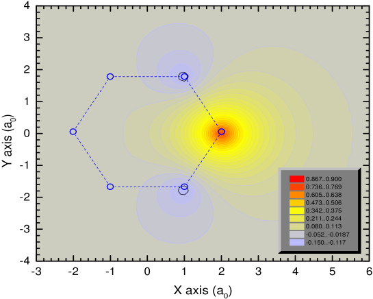
Figure 4: Spatial wave-function profiles for a selected site of $H_{6}$ cluster of hexagonal shape. Note the negative value on the neighboring site to the central atom.

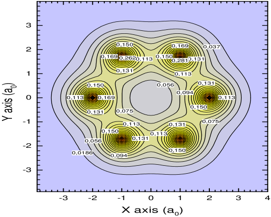
Figure 5: Exact density profiles for electrons in a hexagonal ring of atoms.

An interesting feature of the spectrum of electronic states arises when the distance between the atoms increases. Namely, the spectrum decomposes into well defined Hubbard subbands, as shown in Fig. 6 (more appropriately, they represent manifolds corresponding to the subbands when $N\rightarrow\infty$). The lowest manifold (I) corresponds to the configuration with approximately singly occupied orbitals (highest occupied Wannier orbitals) whereas the manifolds II-IV correspond respectively to the states with one to three double occupancies. This division into the well separated manifolds for larger $R$ is even better seen for the clusters of $N=4$ and 5 atoms [8]. One should mention that the states considered here represent the excited states calculated with the help of Lanczos procedure [5], repeated many times until the configuration with the minimal energy and the optimal single-particle wave function size are reached simultaneously.

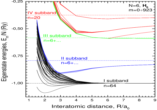
Figure 6: Decomposition of the system energies into Hubbard subbands for $H_{6}$ cluster, plotted as a function of interatomic distance. The horizontal lines represent the atomic limit values for the levels $\frac{Ul}{N}$, with $l=0,1,2,$ and $3$.

5 Further features of the results: collective properties of nanochains

5.1 One electron per atom case: localization threshold

$a/a_{0}$	$D^{*}_{14}$	$D^{*}_{12}$	$D^{*}_{10}$	$D^{*}_{8}$	$D^{*}_{6}$	$D^{*}_{\infty}$	$\sigma(D_{\infty}^{*})/D_{\infty}^{*}$
1.5	0.9225	0.9420	0.9563	0.9727	0.9822	0.8008	0.019
1.6	0.8879	0.9162	0.9378	0.9612	0.9754	0.7175	0.029
1.7	0.8419	0.8817	0.9130	0.9459	0.9667	0.6148	0.043
1.8	0.7826	0.8365	0.8805	0.9256	0.9552	0.4967	0.064
1.9	0.7095	0.7794	0.8389	0.8992	0.9406	0.3728	0.092
2.0	0.6245	0.7105	0.7875	0.8660	0.9222	0.2567	0.129
2.1	0.5315	0.6310	0.7265	0.8254	0.8996	0.1606	0.172
2.2	0.4338	0.5431	0.6549	0.7755	0.8714	0.0899	0.228
2.3	0.3403	0.4523	0.5766	0.7179	0.8379	0.0455	0.287
2.4	0.2554	0.3631	0.4937	0.6524	0.7982	0.0207	0.352
2.5	0.1839	0.2812	0.4109	0.5813	0.7526	0.0087	0.420
2.6	0.1269	0.2096	0.3315	0.5065	0.7009	0.0033	0.489
2.7	0.0840	0.1508	0.2595	0.4312	0.6441	0.0012	0.566
2.8	0.0536	0.1049	0.1972	0.3586	0.5836	0.0004	0.641
2.9	0.0315	0.0706	0.1456	0.2914	0.5208	0.0001	0.920
3.0	0.0196	0.0461	0.1047	0.2314	0.4575	0.0000	$\ \ \ -$

Table 3: Normalized Drude weight $D_{N}^{*}$, the extrapolated value $D_{\infty}^{*}$, and its relative error for 1D half–filled system with long–range Coulomb interactions.

In the previous Sections we illustrated the applications of the EDABI method, in which the interaction among particles is dealt with first. This is because, in most cases, the interaction parameters (coupling constants) represent the largest energy scale in the system. The first of the examples (the Hubbard chain) represents the situation, for which an analytic expression for the ground state energy exists [12], whereas the case of $H_{N}$ rings must be treated numerically all the way through [18]. In applications of this method to the extended three-dimensional systems one will have to resort to the approximate treatments of the model Hamiltonian in the Fock space. This last problem poses a real challenge for the future. In the remaining part of this brief review we concentrate on the collective properties of the nanochain.
We have concentrated first on the basic quantum-mechanical features of the system such as the ground-state energy or the renormalized single-particle wave function in the milieu of other particles. In Fig. 7 we plot the exact ground state energy of a chain of $N=6\div 10$ atoms and compare it with that obtained in the Hartree-Fock approximation for the Slater antiferromagnetic state. The starting Hamiltonian is of the form (10). As one can see the Hartree-Fock energy represents an upper estimate, as it should be. Additionally, the curve M represents the ”metallic” approximation, for which the correlation function $<\delta n_{i}\delta n_{j}>$ has been taken for the 1D electron gas on the lattice. On the contrary, INS represents the energy of the Heisenberg-Mott state in the mean-field approximation. The state of the system crosses over from the Slater metallic-type state to the localized-spin-type of state. This is seen explicitly when we calculate the evolution of the spin-spin correlation function with the increasing interatomic distance, as displayed in Fig. 8. Well defined oscillations of $<{\bf S}_{i}\cdot{\bf S}_{j}>$ are seen for even ($N=12$) number of atoms, which become more pronounced with the increasing $N$ (the frustration effects appear for odd $N$). What is much more important, the autocorrelation part $<{\bf S}_{i}\cdot{\bf S}_{i}>=<{\bf S}_{i}^{2}>=(3/4)(1-2<n_{i\uparrow}n_{i\downarrow}>)$ evolves from the value close to the free-electron value $<{\bf S}_{i}^{2}>=(3/4)(1-2<n_{i\uparrow}><n_{i\downarrow}>)=3/8$ to the atomic-limit value $<{\bf S}_{i}^{2}>=(1/2)(1/2+1)=3/4$. This evolution provides a direct evidence of the crossover from delocalized to the localized regime.

Figure 7: Ground state energy per atom vs. R for the linear chain with $N=6\div 10$ atoms with periodic boundary conditions. The STO-3G Gaussian basis for representation of atomic orbitals forming the Wannier function has been used. The inset provides a universal behavior of the inverse size $\alpha$ of the orbitals. For details see main text.

Figure 8: Spin-spin correlation function $\langle{\bf S}_{i}\cdot{\bf S}_{j}\rangle$ vs. the distance $|i-j|$ between the atomic sites, for different lattice constant $R$ and for $N=12$ atoms. Due to periodic boundary conditions only the distance up to $|i-j|=6$ is relevant. The continuous line is guide to the eye. A quasi-antiferromagnetic arrangement is clearly seen, particularly for larger $R$.

Figure 9: Evolution of the statistical momentum distribution $n_{k\sigma}$ with the increasing interatomic distance $R$. For the nanochain of $N=6,10,$ and $14$ the periodic boundary conditions provide the energy minimum, whereas for $N=8$ and $12$ antiperiodic boundary conditions are appropriate. For details see main text.

Figure 10: Luttinger–liquid scaling for a half–filled 1D chain of $N=6\div 14$ atoms with long–range Coulomb interactions: $(a)$ momentum distribution for electrons in the linear and $(b)$ log–log scale, continuous lines represent the fitted singular expansion in powers of $\ln(\pi/|k_{F}-k|a)$ (see main text for details); $(c)$ Tomonaga–Luttinger model exponent $\theta$ vs. lattice parameter $a$ (specified in $a_{0}$) and (in the inset) the corresponding residual sum of squares. The solid lines in Figures $(a)$ and $(b)$ represent the TLM fitting of Eq. (16).

Other properties such as the electrical conductivity [16] and the statistical distribution in momentum space ($n_{k\sigma}$) have also been addressed [9]. Here the question emerges whether the quantum nano-liquid of electrons in a nanochain resembles at all the Landau-Fermi liquid or if it is rather represented by the Tomonaga-Luttinger scaling laws [17]. The answer is not yet settled, as within our method we can deal only with up to N=16 hydrogen atoms assembled into a linear chain. However, one can make some definite statements for the particular cases. Namely, for the half-filled case (one electron per atom) the modified Fermi distribution is a good representation of the $n_{k\sigma}$ for smaller $R$ values; with the increasing atom spacing it is smeared out above critical spacing $R=R_{c}\approx 3.4a_{0}$ [10], which characterizes a crossover from the case with extended states to the state of localized electrons on atoms, as detailed below. In Fig. 9 we exhibit this evolution on the example of the distribution function (i.e. electron occupation in the momentum space); a clear universality is observed for $N=6\div 14$ atoms. The adjustable Gaussian (STO-3G) single-particle basis has been used in the analysis. The existence of the Fermi ridge quasi-discontinuity for a small $R$ is very suggestive in this case and is positioned near the Fermi wave-vector $k_{F}^{\infty}=\pm\pi/(2R)$, corresponding to that in Landau-Fermi liquid, with $N\rightarrow\infty$. For $N=6,10,14$ periodic boundary conditions (PBC) provide the minimal ground state energy, whereas for $N=8$ and $12$ the anti-periodic boundary conditions (ABC) lead to the lower energy. However, one clearly sees the absence of the points at the Fermi momentum $k_{F}^{\infty}$. This is because, for example, the Fermi points for $N=14$ are located at $k_{F}R/\pi=\pm 3/7$, whereas they are located at $k_{F}R/\pi=\pm 5/12$ for $N=12$, close to the values $\pm 1/2$ in both cases. One would have to apply a renormalization group approach [19] for the states close to $k_{F}$ (i.e. perform the analysis for larger number $N\sim 10^{2}$ atoms) to determine the precise evolution of the distribution function, this time with the system size $N$. Nevertheless, the results for $N\leq 14$ atoms represent those for a true nanoscopic system.
Before addressing the question of localization directly, we would like to address the question whether the computed distribution displayed in Fig. 9 can be fitted into the Tomonaga-Luttinger mode, with the logarithmic scaling corrections included [17]. The statistical distribution near the Fermi point can be represented by

$$\ln|n_{k\sigma}-n_{F}|=-\theta\ln z+b\ln\ln z+O(1/\ln z),$$ (16)

with $z\equiv\pi/|k-k_{F}|$. Here $\theta$ is a non-universal (interaction-dependent) exponent (it yields the nonexistence of fermionic quasiparticles, since its residue vanishes as $Z_{k}\sim|k-k_{F}|^{\theta}$ with $k\rightarrow k_{F}$. The corresponding electron-momentum distribution is depicted in Fig. 10a in the linear, and in Fig. 10b in the log-log scale. The $R$ dependence of the exponent $\theta$ is shown in Fig. 10c and crosses the value $\theta=1$ for $R=R_{c}\approx 2.6a_{0}$ corresponding to the localization threshold [17]. This threshold is about 30% smaller than the corresponding value ($R_{c}\approx 3.4a_{0}$) when the almost-localized Fermi-liquid view was taken [10]. One should also note that the Luttinger scaling does not reproduce well the occupancies farther away either way from the Fermi point. Thus the results concerning $n_{k\sigma}$ do not provide a definite answer as to the exact nature of the nanoliquid composed of $N\sim 10$ electrons, although it is absolutely amazing that they have such a nice and simple scaling properties.
To address the question of the electron localization directly, we have calculated the optical conductivity $\sigma(\omega)$, which can be written in the form $\sigma(\omega)=D\delta(\omega)+\sigma_{reg}(\omega)$, where the regular part is

$$\sigma_{reg}(\omega)\frac{\pi}{N}\sum_{n\neq 0}\frac{|<\Psi_{n}|j_{p}|\Psi_{0}>|^{2}}{E_{n}-E_{0}}\delta(\omega-(E_{n}-E_{0})),$$ (17)

whereas the Drude weight (the charge stiffness) $D$ is given by

$$D=\frac{\pi}{N}<\Psi_{0}|T|\Psi_{0}>-\frac{2\pi}{N}\sum_{n\neq 0}\frac{|<\Psi_{n}|j_{p}|\Psi_{0}>|^{2}}{E_{n}-E_{0}},$$ (18)

with $T$ being the hopping term as in (9) and $j_{p}$ the current operator defined as $j_{p}=it\sum_{ij\sigma}(a^{\dagger}_{j\sigma}a_{i\sigma}-h.c.)$. Here $|\Psi_{n}>$ is the system eigenstate corresponding to the eigenvalue $E_{n}$. For a finite system of N atoms D is always nonzero due to nonzero tunnelling rate through a potential barrier of finite width. Because of that, the finite-size scaling with $1/N\rightarrow 0$ must be performed on $D$. We use the following parabolic extrapolation

$$\ln D^{\star}_{N}=a+b(1/N)+c(1/N)^{2},]$$ (19)

where $D^{\star}_{N}=-(N/\pi)D/<\Psi_{0}|T|\Psi_{0}>$ denotes the normalized Drude weight for the system of N sites. We observe that $0\leq D^{\star}\leq 1$ and hence can be regarded as an order parameter for the transition to the localized (atomic) states. In Table 3 we plot the weights $D^{\star}_{N}$, the extrapolated values $D^{\star}_{\infty}$, and its relative error for 1D half-filled system with long-range Coulomb interactions included. What is very important, the value of $D^{\star}_{N}$ drops by two orders of magnitude when R changes by a factor of two (between $1.5a_{0}$ and $3a_{0}$). Note also that $D^{\star}_{\infty}$ is within its error for $R\simeq R_{c}\approx 2.3a_{0}$, close to the value obtained from the Tomonaga-Luttinger scaling for $n_{k\sigma}$, as one would expect. The result for $D^{\star}_{N}$ is probably telling us how far we can go quantitatively when discussing the localization in nanowires. These results will be detailed in a separate publication.

5.2 Quarter-filled case

Figure 11: Momentum distribution $n_{k\sigma}$ for electrons on a chain of $N=8\div 16$ atoms in the quarter–filled band case ($N_{e}=N/2$). Lines are drawn as a guide to the eye only. Values of the lattice parameter $R$ are specified in units of $a_{0}$. PBC and ABC denote periodic and antiperiodic boundary conditions, respectively. The dashed line marks occupation $n_{k\sigma}=1/2$.

Figure 12: Charge–density distribution for the quarter–filled ($N_{e}=N/2$) nanochain as viewed by density–density fluctuation correlation function $\left<\Delta n_{i}\Delta n_{j}\right>$ vs. relative distance $\left|i-j\right|$.

For the quarter-filled case (i.e. when every second atom contributes a valence electron) the distribution ${n}_{{\bf k}\sigma}$ is more smeared out, as shown in Fig. 11. The ground state for $R\geq 3a_{0}$ is then well represented by the charge-density-wave state, since then the density-density correlation function $\langle(n_{i}-\overline{n})(n_{j}-\overline{n})\rangle$ exhibits the oscillatory behavior, as shown in Fig. 12. The onset of the charge-density wave state in that case is invariably due to the long-range Coulomb interaction $\sim K_{ij}$, which is reduced in that state. The charge-density wave order parameter defined as

$$\Theta_{CDW}\equiv\frac{1}{N}\sum_{m}(-1)^{m}<(n_{i}-\overline{n})(n_{j}-\overline{n})>$$ (20)

reaches its maximal value $1/4$ for $R\geq 8a_{0}$. Let us stress again, the form of the statistical distribution (and its feasibility) for $N\sim 10$ atoms is a very interesting question by itself, since this is the regime of nanoscience. Our results show that even in that regime one should be able to see the signatures of the phase transition to the spin- or charge- density wave states.

6 Conclusions

The EDABI method (Exact Diagonalization combined withAB Initio orbital readjustment)provides the exact ground state energy of the model systems considered (Hubbard chain, nanoscopic chains and rings) as a function of interatomic distance. It also provides reliably other ground-state dynamical characteristics for nanoscopic systems: spin and charge correlation functions, the spectral density and the density of states, as well as the system conductivity. Not all the characteristics have been presented in this overview [5, 10, 16, 17]. Furthermore, the method can also be extended to nonzero temperatures. Finally, it should be underlined again that our method of approach is particularly suited for strongly correlated systems, where the interaction and the single-particle parts should be treated on the same footing. The exact numerical results in a model situation can also serve as a test for approximate analytic treatments.
The analysis with inclusion of long-range Coulomb interactions of the distribution function $n_{k\sigma}$ in either Fermi-like or Tomonaga-Luttinger categories suggests the existence of the crossover transition to the localized state with the increasing interatomic distance $R$. This state is either the spin- or the charge- ordered for the number of electrons $N_{e}=N$ and $N/2$, respectively. In the small $R$ limit the state can be rendered as quasi-metallic in the sense that the quasimomentum $\hbar k$ can be regarded as a good quantum number, even though the level structure is discrete. The difference between the short-chain and infinite-chain situation is due to the circumstance that in order to form extended states in the present case the electrons tunnel through a barrier of finite width (the length $L=NR$). This is one of the reasons for quasi-metallicity. The other is the presence of the long-range Coulomb interaction[20].

7 Acknowledgment

The work was supported by the State Committee for Scientific Research KBN, Grant No. 2P03B 050 23. The two authors (A.R & J.S.) acknowledge respectively the junior and the senior fellowships of the Foundation for Science (FNP). We are also grateful to the Institute of Physics of the Jagiellonian University for the support for computing facilities used in part of the numerical analysis.

xxx

References

- [1] P.C. Hohenberg, W. Kohn, and L.I. Sham, in Adv. Quantum Chemistry, edited by S.B. Trickey (Academic, San Diego, 1990) vol. 21, pp. 7-26; W. Temmerman et al., in Electronic Density Functional Theory: Recent Progress and New Directions, edited by J.F. Dobson et al. (Plenum, New York, 1998) pp. 327-347.
- [2] V.I Anisimov, J. Zaanen, and O.K. Andersen, Phys. Rev. B 44, 943 (1991); P. Wei and Z.Q.Qi,ibid. 49, 10864(1994).
- [3] A. Svane and O. Gunnarson, Europhys. Lett. 7, 171 (1988); Phys. Rev. Lett. 65, 1148(1990)
- [4] S. Ezhov et al., Phys. Rev. Lett. 83, 4136(1999); K. Held et al., ibid. 86, 5345 (2001).
- [5] J. Spałek et al., Phys. Rev. B 61, 15676 (2001); A. Rycerz and J. Spałek, ibid. B 63, 073101(2001); B 65, 035110(2002); J Spałek et al., submitted to Phys. Rev. B.
- [6] J. Spałek et al., Acta Phys. Polonica B 31, 2879(2000); ibid., B 32, 3189 (2001).
- [7] A. Rycerz et al., in Lectures on the Physics of Highly Correlated Electron Systems VI, edited by F. Mancini, (AIP Conf. Proc. No. 629, New York, 2002) pp. 213-223; ibid. (AIP Conf. Proc. No. 678, New York, 2003) pp. 313-322.
- [8] J. Spałek et al., in Concepts in Electron Correlation, Proc. of the NATO Adv. Res. Workshop, edited by A.C. Hewson and V. Zlatić (Kluwer, Dordrecht, 2003) pp. 257-268.
- [9] J. Spałek et al., in Highlights of Condensed Matter Physics, (AIP Conf. Proc. No. 695, New York, 2003)pp. 291-303.
- [10] J. Spałek and A. Rycerz, Phys. Rev. B 64, 161105 (2001)(R).
- [11] If we want to include it, then it is irrelevant for the case of one electron per atom, since then pure spin-density-wave correlations set in. However, if the system is non-neutral (), then the charge-density-wave state may become stable (c.f. Fig. 12 in Sec. 5).
- [12] E.H. Lieb and F.Y. Wu, Phys. Rev. Lett. 20, 1443(1968). For overview see: M. Takahashi, Thermodynamics of one-dimensional solvable models (Cambridge Univ. Press, 1999) ch. 6.
- [13] M.C. Gutzwiller, Phys. Rev. 137, A1726(1965) and references therein.
- [14] W. Metzner and D. Vollhardt, Phys. Rev. B 37, 7382 (1988).
- [15] J. Spałek, J. Kurzyk, W. Wójcik, E.M. Görlich, and A. Rycerz, submitted for publication.
- [16] A. Rycerz, Ph. D. Thesis, Jagiellonian University, Kraków - 2003 (unpublished).
- [17] J. Solyom, Adv. Phys. 28, 201(1979); J. Voit, Rep. Prog. Phys. 57, 977(1995).
- [18] R. Zahorbeński and J. Spałek, unpublished.
- [19] S.R. White, Phys. Rep. 301, 187 (1998); R. Shankar, Rev. Mod. Phys. 66, 129 (1994)
- [20] D. Poilbanc et al., Phys. Rev. B 56, R1645(1997).