Dynamical systems with time-dependent coupling: Clustering and critical behaviour

Abstract

We study the collective behaviour of an ensemble of coupled motile elements whose interactions depend on time and are alternatively attractive or repulsive. The evolution of interactions is driven by individual internal variables with autonomous dynamics. The system exhibits different dynamical regimes, with various forms of collective organization, controlled by the range of interactions and the dispersion of time scales in the evolution of the internal variables. In the limit of large interaction ranges, it reduces to an ensemble of coupled identical phase oscillators and, to some extent, admits to be treated analytically. We find and characterize a transition between ordered and disordered states, mediated by a regime of dynamical clustering.

and

1 Introduction

Large ensembles of coupled dynamical systems are a basic tool for the study of emergent collective behaviour in systems of interacting agents [1]. Self-organization in spatially distributed ensembles is revealed by the appearance of spatiotemporal structures, which may exhibit complex evolution. Instead, coupled ensembles for which space is not relevant to the dynamical laws become organized in temporal patterns, typically, in some form of synchronous evolution. Much attention has been focused on synchronization phenomena over the last years [2]. They have been identified in a broad class of natural and artificial systems, and many of them have been successfully explained by means of relatively simple models.

The degree of collective organization in a coupled ensemble, measured by the correlation between individual motions, varies considerably between different kinds of synchronization patterns. Most studies on these phenomena have dealt with patterns of highly correlated evolution, such as full and phase synchronization. Indeed, these forms of synchronization are essential to the functioning of some artificial systems, and have been observed in certain insect populations [3, 4]. On the other hand, they are expected to play a less relevant role in most biological systems, where the complexity of collective functions requires a delicate balance between coherence and diversity [1]. Consider, for instance, the brain, where highly coherent activity patterns are only realized under pathological states, such as during epileptic seizures. Many biological systems consisting of interacting agents, ranging from biomolecular complexes to social populations, are normally found in configurations where the ensemble is segregated into groups with specific functions. While the evolution of individual elements is highly correlated inside each group, the collective dynamics of different groups is much more independent. Clustering has been modeled by means of coupled ensembles with specific individual dynamics or interactions [5, 6, 7, 8, 9].

Usually, clustering is a dynamical process, where groups may preserve their identity in spite of the fact that single elements are continuously migrating between them. Intermittent formation of clusters and migration of elements has been observed under the action of noise [10, 11, 12]. The individual motion towards or away from clusters may also be controlled by the internal state of each element, which favors or inhibits grouping with other elements. This is observed in natural phenomena ranging from complex chemical reactions, where biomolecules react with each other only when they have reached appropriate internal configurations [13], to social systems, where the appearance of organizational structures requires compatibility between the individual changing states of the involved agents [14]. Focusing on this motivation, in this paper we study a model of coupled motile elements where interactions depend on the internal state of each element. Individual internal variables change with time according to a prescribed autonomous evolution law, so that interactions are also time-dependent, and result to be alternatively attractive or repulsive. This intricate interaction pattern induces several complex regimes of collective evolution, including dynamical clustering. Clustering in systems of interacting moving particles with internal dynamics has been demonstrated when the internal states of different elements are mutually coupled and their individual evolution is chaotic [15]. In such case, the synchronization of internal variables results into spatial organization, through the effect of those variables on the degrees of freedom associated with motion. Here, we show that similar forms of collective behaviour are already possible with simple, autonomous oscillatory dynamics for the internal variables.

In the next section, we introduce the model and present numerical results for the case of two-dimensional motion in a bounded domain. The occurrence of different dynamical regimes is controlled by the range of interactions and by the dispersion in the time scales associated with the internal dynamics. In Section 3, the limit of large interaction ranges is analyzed. In this limit, the system reduces to an ensemble of identical phase oscillators with internal states. As the dispersion in the time scales of internal variables is varied, it exhibits an order-disorder transition between a configuration where the phase and the internal variable are highly correlated and a uncorrelated state. This critical transition, which we are able to describe analytically, is mediated by a regime of dynamical clustering. Both the transition and the clustering regime are characterized by means of suitably defined order parameters. In the final section, we discuss our results with emphasis in the features that might be also observed in other systems of similar kinds.

2 Dynamical clustering of motile elements

2.1 Model

We consider an ensemble of $N$ motile elements at positions ${\bf r}_{i}$ ($i=1,\dots,N$). The elements interact through pair forces ${\bf F}({\bf r}_{i}-{\bf r}_{j})$ depending on their relative positions. Moreover, the interaction of each pair is modulated by a function $V(\theta_{i},\theta_{j})$ of the variables $\theta_{i}$ and $\theta_{j}$, which characterize the internal state of the respective elements. This modulation aims at describing the effects of the internal states on the spatial dynamics. The motion of the elements is assumed to be overdamped, so that the equation of motion for element $i$ is

$$\dot{\bf r}_{i}=\sum_{j\neq i}V(\theta_{i},\theta_{j}){\bf F}({\bf r}_{i}-{\bf r}_{j}).$$ (1)

From the viewpoint of the numerical resolution of Eqs. (1), a convenient choice for the interactions a truncated elastic force,

$${\bf F}({\bf r}_{i}-{\bf r}_{j})=\left\{\begin{array}[]{ll}-k({\bf r}_{i}-{\bf r}_{j})&\mbox{ if $|{\bf r}_{i}-{\bf r}_{j}|<r_{0}$,}\\ 0&\mbox{ otherwise.}\end{array}\right.$$ (2)

Here, $k>0$ is the elastic constant and $r_{0}$ is the interaction range.

As for the internal state described by the variable $\theta_{i}$, we assume that each element behaves as an autonomous oscillator with constant frequency $\Omega_{i}$, much like a “biological clock.” Biological periodic phenomena at several levels, from intracellular chemical reactions to complex long-period rhythms, are in fact well described by such elementary cyclic processes [16]. The internal variable represents thus a phase, and evolves in time as

$$\theta_{i}(t)=\Omega_{i}t+\theta_{i}(0).$$ (3)

To take into account inhomogeneity in the ensemble, the frequencies $\Omega_{i}$ are drawn from a given distribution $g(\Omega)$. Here, we take the Gaussian

$$g(\Omega)=\frac{1}{\sqrt{2\pi\sigma^{2}}}\exp\left[-\frac{(\Omega-\Omega_{0})^{2}}{2\sigma^{2}}\right].$$ (4)

The autonomous dynamics of the internal phases $\theta_{i}$ represents cyclic processes which, in our model, are not influenced by external factors but affect the interaction between elements. Specifically, the interaction weight $V(\theta_{i},\theta_{j})$ in Eq. (1) is chosen as

$$V(\theta_{i},\theta_{j})=\cos(\theta_{i}-\theta_{j})=\cos[(\Omega_{i}-\Omega_{j})t+\theta_{ij}^{0}],$$ (5)

with $\theta_{ij}^{0}=\theta_{i}(0)-\theta_{j}(0)$. With this choice, the interaction between elements $i$ and $j$ changes its sign periodically, in a time scale of order $(\Omega_{i}-\Omega_{j})^{-1}$. Thus, it is alternatively attractive or repulsive, respectively favoring or inhibiting the aggregation of elements. At the level of the whole ensemble, this variations give rise to a complex time-dependent interaction pattern which, as shown below, induces a variety of dynamical regimes, including dynamical clustering. Note that, according to Eq. (5), interactions between pairs of elements do not depend separately on the individual frequencies, but on the frequency differences $\Omega_{i}-\Omega_{j}$. Thus, in Eq. (4), we can fix $\Omega_{0}=0$.

As a final ingredient of the model, it is necessary to consider that the ensemble is confined within a bounded spatial domain. In fact, when mutually attracting elements have aggregated into clusters, we expect that the remnant repulsion between elements in different neighbor clusters drives them away from each other. In the long run, this effect would lead to the total dispersion of the ensemble. Therefore, we assume that the system evolves into a closed domain with reflecting boundaries.

2.2 Numerical results

We have extensively studied the above model, by solving Eqs. (1) numerically for a two-dimensional system, where an ensemble of $N=100$ elements is confined within a circle of radius $r_{\max}$. Simultaneous rescaling of frequencies and time makes it possible to fix the elastic constant to $k=1$. Moreover, we choose $r_{\max}$ as the unit of distance. In this way, the only relevant parameters in the model are the interaction range $r_{0}$ and the frequency dispersion $\sigma$.

Truncation errors in the numerical resolution of the equations of motion (1) may cause that, under the effect of attractive interactions, two elements collapse to numerically indistinguishable positions. This is expected to happen, in particular, when the evolution of internal phases is slow (small $\sigma$) so that attractive interactions can act during sufficiently long times. Under such conditions, in view of Eq. (2), the mutual interaction of the collapsed elements will vanish, and the forces applied on each of them by any other element will be identical. Consequently, the collapsed elements will remain “stuck together” for the remaining of the evolution. To avoid this numerical artifact, we introduce in Eqs. (1) a small additive-noise term which prevents the spatial collapse of elements and, otherwise, does not affect the dynamics.

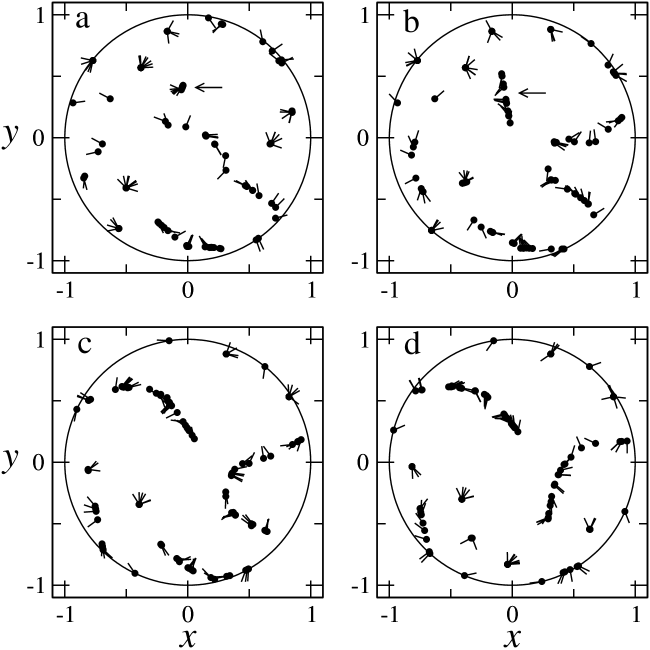
Figure 1: Four snapshots of an ensemble of size $N=100$, with $r_{0}=0.3$ and $\sigma=0.1$, at times (a) $t=5100$, (b) $t=5110$, (c) $t=5120$, and (d) $t=5130$. Each dot represents the position ${\bf r}_{i}=(x_{i},y_{i})$ of an element on the plane, while the orientation of the stick starting at each dot indicates the value of the corresponding internal phase $\theta_{i}$. Circles show the system boundary. All the elements of the cluster marked with an arrow in (a) are part of the “string” marked in (b).

Figure 1 shows four successive snapshots of the ensemble, in a single realization with $r_{0}=0.3$ and $\sigma=0.1$. We find that many elements are entrained in several compact clusters, while others are distributed in space along curved lines, forming “strings.” These “strings” result from the instabilization of clusters, as illustrated in Figs. 1a and b. Generally, the distribution of internal phases $\theta_{i}$ of the elements belonging a given cluster spans a total angle less than $\pi$, but this total angle is often larger than $\pi/2$. This implies that, inside a cluster, the difference of internal phases between a pair of elements can be larger than $\pi/2$, and their interaction can thus be repulsive. However, the two elements can be part of the same cluster due to the presence of other elements with intermediate internal phases. These elements mediate the interaction between the otherwise repulsive pairs, in such a way that the effective force is attractive towards the cluster.

Once a cluster is formed, and after a certain transient has elapsed, the total angle spanned by the distribution of internal phases $\theta_{i}$ grows with time, due to the individual evolution of each phase, Eq. (3). This growth takes place within time scales of order $\min_{ij}|\Omega_{i}-\Omega_{j}|^{-1}$. Under some simplifying assumptions, it can be shown that a cluster becomes unstable when the total angle spanned by the internal phases reaches $\pi$. Suppose that, at a given moment, the internal phases of the $n$ elements belonging to a cluster are uniformly distributed over the interval $(0,\Theta)$. Suppose also that all the elements are at the same point in space, except for a test element at a small distance $\delta{\bf r}$ (with $|\delta{\bf r}|<r_{0}$) from the cluster. If $n$ is sufficiently large, taking into account Eqs. (1) to (5), the equation of motion of the test element can be written as

$$\delta\dot{\bf r} = -k\,\delta{\bf r}\sum_{i}\cos(\theta_{i}-\theta_{0})\approx k\,n\,\delta{\bf r}\ \frac{1}{\Theta}\int_{0}^{\Theta}\cos(\theta_{0}-\theta)d\theta=$$ (6)

$$= k\,n\,\frac{\sin(\theta_{0}-\Theta)-\sin\theta_{0}}{\Theta}\,\delta{\bf r},$$

where $\theta_{0}$ is the internal phase of the test element. The factor multiplying $\delta{\bf r}$ in the right-hand side of Eq. (6) is negative for all $\theta_{0}\in(0,\Theta)$ if $0\leq\Theta<\pi$. Under these conditions, the force on the test element is attractive. As $\Theta$ reaches $\pi$, however, the factor of $\delta{\bf r}$ becomes positive at $\theta_{0}=0$ and $\pi$. This implies that, as soon as $\Theta>\pi$, the elements with extreme internal phases, $\theta\approx 0$ or $\theta\approx\pi$, will be repelled from the cluster. Due to their mutual repulsion, elements with internal phases close to $\theta=0$ and $\theta=\pi$ will move away from the cluster in opposite directions. Moreover, as the distribution of phases in the remaining of the cluster keeps broadening and new elements reach the stability limits, they will be attracted by those elements with similar phases which have just left the cluster, and therefore move in their direction. This mechanism gives rise to the “strings” of elements when a cluster becomes unstable and disintegrates.

The dynamics of clustering is effectively illustrated by the distribution of distances between elements [6, 7]. Calculating the $N(N-1)/2$ Euclidean pair distances

$$d_{ij}=|{\bf r}_{i}-{\bf r}_{j}|$$ (7)

for all $i$ and $j>i$, we construct a histogram where the height of the column with base $(d,d+\Delta d)$ is proportional to the number of pair distances within that interval. Compact clusters cause the appearance of sharp peaks in the histogram, at $d\approx 0$ and other distances, while non-clustered elements give rise to a smooth background. Figure 2 shows, as a density plot, the evolution of a $200$-column histogram of pair distances $d\in(0,2)$ ($\Delta d=0.01$) for the same numerical realization as in Fig. 1, between $t=9800$ and $10000$. As expected, the region $d<r_{0}$ is strongly depleted (except for the peak at $d\approx 0$), because pairs of elements at such distances either become entrained into clusters or are mutually repelling. For $d>r_{0}$, dark horizontal lines reveal localized compact clusters. As time elapses, these clusters can become less well-defined, and they are seen to move, disperse, coalesce, or split to form smaller groups.

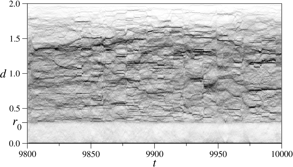
Figure 2: Density plot of the histogram of pair distances as a function of time, for the same realization as in Fig. 1 ($N=100$, $r_{0}=0.3$, $\sigma=0.1$), along $200$ time units. Darker tones correspond to higher concentrations.

This complex dynamics, driven by the autonomous evolution of the internal phases, calls for a statistical description in terms of a characterization of the partition of the ensemble into clusters. With this aim, we introduce two order parameters [6]. The parameter $R$ is the time-averaged fraction of pair distances smaller than a certain small threshold $\delta$. It reads

$$R=\left\langle\frac{2}{N(N-1)}\sum_{i=1}^{N}\sum_{j=i+1}^{N}H(\delta-d_{ij})\right\rangle,$$ (8)

where $\langle\cdot\rangle$ indicates average over long times, and $H(z)$ is the step function: $H(z)=1$ for $z>0$, and $H(z)=0$ otherwise. The second parameter, $S$, is given by the time-averaged fraction of elements which have at least another element as a distance smaller than $\delta$. It can be calculated as

$$S=\left\langle 1-\frac{1}{N}\sum_{i=1}^{N}\prod_{j=i+1}^{N}H(\delta-d_{ij})\right\rangle.$$ (9)

Associating the threshold $\delta$ with the (maximal) size of a cluster, both parameters are statistical measures of the degree of clustering in the ensemble. Their values are close to zero if most elements are not entrained, and reach unity if all elements belong to clusters. They are, however, independent quantities. For a fixed value of $S$, which measures the total population inside clusters, $R$ is small if the number of clusters is large, and vice versa. In other words, $R$ characterizes the average number of elements per cluster. An approximate evaluation of the number of clusters $M$ is obtained by assuming that all clusters have the same population, as $M=S^{2}/R$ [6].

To characterize clustering in our system, we have numerically calculated the order parameters $R$ and $S$ as functions of the frequency dispersion $\sigma$ and the interaction range $r_{0}$ in a system of $N=100$ elements, taking $\delta=0.01$. Figure 3 shows $R$ and $S$ versus $\sigma$ for $r_{0}=0.3$. For this intermediate value of the interaction range, the two order parameters display a moderate decrease as the frequency dispersion grows. As frequency differences become larger, the typical length of the time intervals during which the interaction of a given pair of elements is attractive shortens. Consequently, shorter times are available for the aggregation of elements into clusters and, thus, the average degree of clustering diminishes. The approximate number of clusters, calculated as $M=S^{2}/R$, is practically constant, $M\approx 20$, in the considered interval of variation for $\sigma$. The same behaviour is found for smaller values of the interaction range. On the other hand, for large values of $r_{0}$, the dependence with the frequency dispersion becomes less trivial. We analyze this specific situation in the next section.

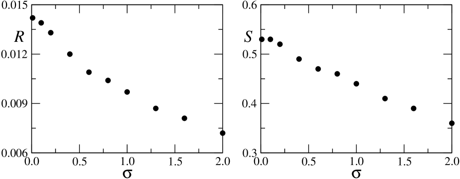
Figure 3: The order parameters $R$ and $S$ as functions of the frequency dispersion $\sigma$, for an interaction range $r_{0}=0.3$.

The dependence of the clustering order parameters $R$ and $S$ on the interaction range $r_{0}$ for fixed $\sigma$ is more interesting, as shown in Fig. 4 for $\sigma=0.1$. We find that both parameters display a maximum, at $r_{0}\approx 0.27$ for $R$ and $r_{0}\approx 0.23$ for $S$. For smaller values of the interaction range, the two parameters rapidly drop to zero, while for larger $r_{0}$ they exhibit a smoother decay. The approximate number of clusters, $M=S^{2}/R$, grows steadily from $M\approx 1$ for $r_{0}\approx 0$ and attains a sharp maximum, $M\approx 30$, at $r_{0}\approx 0.25$. For larger interaction ranges, it soon reaches an almost constant value, $M\approx 20$.

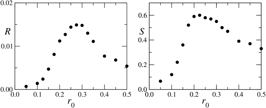
Figure 4: The order parameters $R$ and $S$ as functions of the interaction range $r_{0}$, for a frequency dispersion $\sigma=0.1$.

In order to explain the non-monotonic dependence of the clustering order parameters with the interaction range, it is useful to inspect the instantaneous spatial distribution of the ensemble for different values of $r_{0}$ (Fig. 5). For sufficiently small $r_{0}$, there is little chance that two elements are simultaneously found within the interaction range. In our two-dimensional system, the average distance $\bar{d}$ between elements can be evaluated as $\bar{d}=\sqrt{A/N}$, where $A$ is the area of the domain accessible to the ensemble. Taking $A=\pi r_{\max}^{2}$ and $r_{\max}=1$, we find $\bar{d}\approx 0.18$. Figures 5a and b show that for $r_{0}<\bar{d}$ only a few elements form clusters, whereas for $r_{0}\gtrsim\bar{d}$ most of the ensemble is clustered in many groups. For such values of the interaction range, consequently, the clustering order parameters increase with $r_{0}$ (Fig. 4).

As the interaction range grows, the collective organization of elements in larger spatial structures becomes possible. In particular, the “strings” associated with unstable clusters, discussed above, entrain now a substantial part of the ensemble (Fig. 5c). The contribution of these structures to the clustering order parameters is expected to be considerably weaker than that of compact clusters, which explains the decline of $R$ and $S$ for $r_{0}\gtrsim 0.3$. For even larger interaction ranges the dynamics is dominated by the remnant repulsive interaction between compact clusters. When $r_{0}$ is sufficiently large, all the elements are found most of the time at the boundary of the spatial domain (Fig. 5d). Note that elements are still organized in space according to their internal state: generally, neighbouring elements have similar internal phases. This form of organization in the limit of large interaction ranges is treated in detail in the next section.

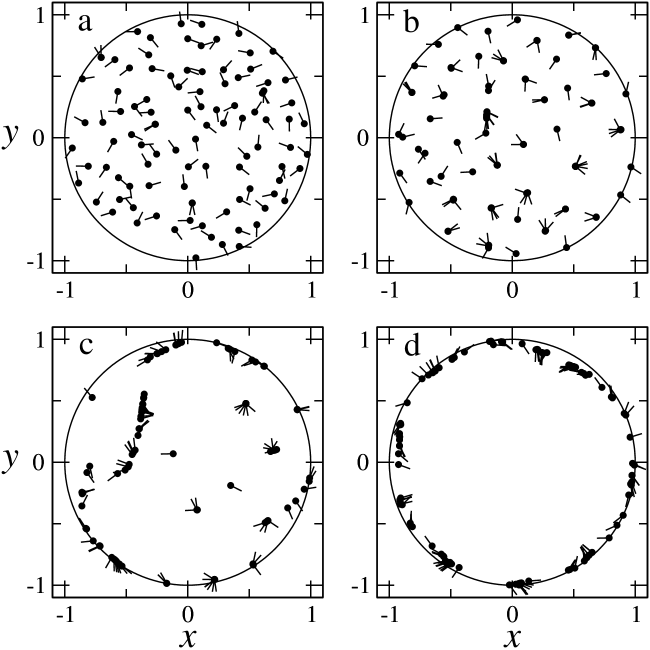
Figure 5: Four snapshots of an ensemble of size $N=100$ at times $t=10000$, with $\sigma=0.1$ and different interaction ranges: (a) $r_{0}=0.1$, (b) $r_{0}=0.2$, (c) $r_{0}=0.3$, and (d) $r_{0}=0.5$.

The change in the collective spatial distribution as the interaction range grows is also apparent in the distribution of pair distances $d_{ij}$. Figure 6 shows $200$-column normalized histograms of pair distances for the snapshots shown in Fig. 5. When the degree of clustering is small (Fig. 6a) the distribution of pair distances is rather smooth, and no significant contributions are present at $d\approx 0$. As the interaction range grows and clustering becomes more important, the distribution spreads and develops sharp spikes. Note, in particular, the high peak at $d\approx 0$ (Fig. 6b and c). For even larger $r_{0}$ the degree of clustering recedes, the peak at $d\approx 0$ becomes smaller, and other spikes are replaced by broader structures (Fig. 6d). The highest peak, centered at $d\approx 1.8$, is a direct byproduct of the concentration of elements in the boundary of the spatial domain.

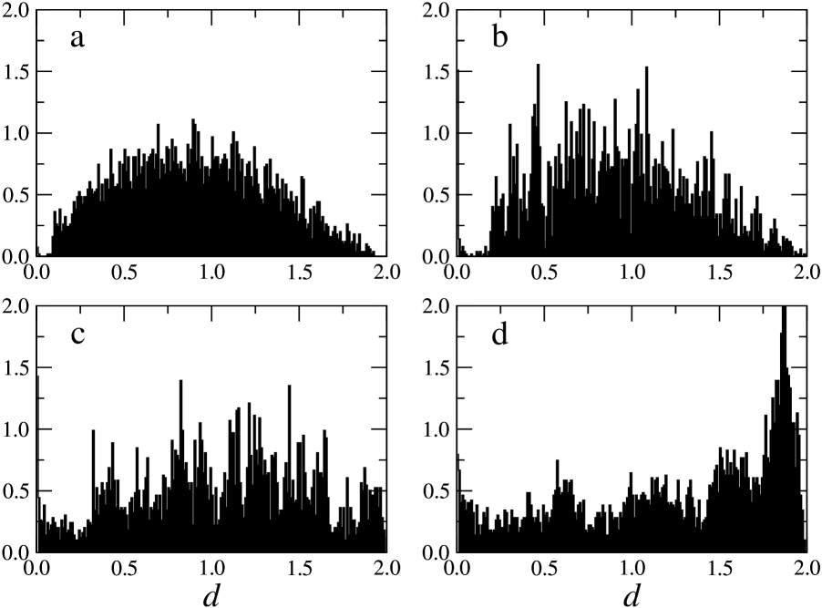
Figure 6: Normalized histograms of pair distances for the snapshots of Fig. 5. (a) $r_{0}=0.1$, (b) $r_{0}=0.2$, (c) $r_{0}=0.3$, and (d) $r_{0}=0.5$.

The fact that, in the limit of large interaction range, the ensemble is mainly concentrated in the boundary of the accessible domain suggest a reduced representation of the problem, where the position of each element is given by a linear coordinate along the boundary. In the case of the circular domain considered above, such approximation yields a set of dynamical equations which are formally equivalent to the model equations of coupled phase oscillators. As shown in the next section, this reduced representation admits to be studied analytically to a considerable extent.

3 Phase oscillators with time-dependent coupling

3.1 Reduction to phase variables

When the range of interactions is larger than the linear size of the system, all the elements are subject to the action of the whole ensemble at all times. As discussed in the preceding section, the regime of large $r_{0}$ is characterized by the repelling interaction of clusters, which drives the elements to the boundaries of the accessible spatial domain. For the case of the circular domain considered above, the position of an element at the boundary can be characterized by the angle $\phi_{i}$ defined by the element and an arbitrarily chosen origin, with vertex at the center of the circle. Assuming that the elements do not abandon the boundary at any time, the evolution of $\phi_{i}$ is governed by

$$\dot{\phi}_{i}=-\dot{x}_{i}\sin\phi_{i}+\dot{y}_{i}\cos\phi_{i}=\sum_{j\neq i}V(\theta_{i},\theta_{j})F_{ij}^{\parallel},$$ (10)

where $F_{ij}^{\parallel}$ is the projection of the pair force ${\bf F}({\bf r}_{i}-{\bf r}_{j})$ parallel the circular boundary [cf. Eq. (1)]. Figure 7 shows the geometry of the problem. With $r_{0}>2r_{\max}=2$, the modulus of the force (2) between any pair of elements is given by

$$F_{ij}=k\,d_{ij}=k\sqrt{2[1-\cos(\phi_{j}-\phi_{i})]}=2k\sin\left(\frac{\phi_{j}-\phi_{i}}{2}\right).$$ (11)

The angle between the force and the tangent to the circle at the position of element $i$ is $(\phi_{j}-\phi_{i})/2$. Therefore,

$$F_{ij}^{\parallel}=F_{ij}\cos\left(\frac{\phi_{j}-\phi_{i}}{2}\right)=k\sin(\phi_{j}-\phi_{i}).$$ (12)

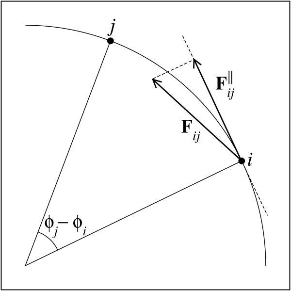
Figure 7: Reduction of the circular-domain problem to phase variables, in the limit of large interaction range.

The equation of motion for $\phi_{i}$ becomes

$$\dot{\phi}_{i}=k\sum_{j\neq i}V(\theta_{i},\theta_{j})\sin(\phi_{j}-\phi_{i}).$$ (13)

Remarkably, this equation is formally equivalent to the model equation for an ensemble of phase oscillators with identical natural frequencies $\omega=0$, where the state of each oscillator is characterized by its phase $\phi_{i}$. The collective behaviour of ensembles of phase oscillators has been thoroughly analyzed during the last two decades. With $V(\theta_{i},\theta_{j})\equiv 1$ for all $i,j$, Eq. (13) reduces to the Kuramoto model for globally coupled identical oscillators [17]. In this case, full synchronization ($\phi_{i}(t)=\phi_{j}(t)$ for all $i,j$) is a stable asymptotic state for any positive value of $k$. Time-independent interaction weights, where $V(\theta_{i},\theta_{j})\equiv V_{ij}$ is constant but can have different values for each oscillator pair, have been shown to induce typical features of disordered systems, such as glassy-like behaviour, frustration, and algebraic relaxation towards equilibrium [18, 19, 20]. As we show in the following, when the interaction between phase oscillators is modulated by the time-dependent interaction weight $V(\theta_{i},\theta_{j})$ defined by Eqs. (3) and (5), various forms of collective evolution –including dynamical clustering– emerge. The transition between these regimes is controlled by $\sigma$, the frequency dispersion of the internal phases $\theta_{i}$, which is now the only parameter left in the model.

3.2 Order-disorder critical transition

We begin our analysis of Eq. (13) by performing numerical simulations of the system for ensembles ranging from $N=10^{2}$ to $10^{6}$. As customary with coupled phase oscillators, we rescale the constant $k$ with the ensemble size as $k=K/N$, and fix $K=1$. The frequencies $\Omega_{i}$ of the internal phases are drawn from the distribution of Eq. (4). We fix $\Omega_{0}=0$, and consider various values of the frequency dispersion $\sigma$. Figure 8 shows snapshots of the ensemble taken at sufficiently long times, for three values of $\sigma$. For small $\sigma$ (Fig. 8a), the phases $\phi_{i}$ are homogeneously distributed around the circle, and a high degree of correlation between $\phi_{i}$ and the internal variables $\theta_{i}$ is apparent. For large frequency dispersion, the distribution of phases is also approximately homogeneous but, on the other hand, the correlation with the internal variables is lost (Fig. 8c). At intermediate values of $\sigma$, we find strongly heterogeneous distributions for the phases $\phi_{i}$. Figure 8b shows a state where most of the ensemble is split into two clusters with opposite phases.

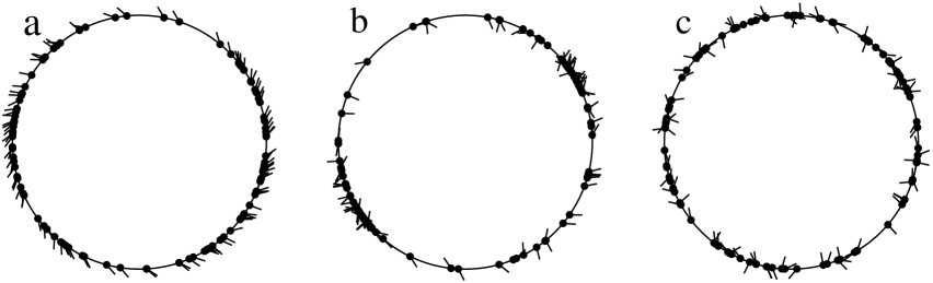
Figure 8: Long-time snapshots of an ensemble of $100$ phase oscillators, for different values of the frequency dispersion: (a) $\sigma=0.1$, (b) $\sigma=0.3$, and (c) $\sigma=0.5$.

To explain the appearance of these three regimes we first note that, for small $\sigma$, the internal variables –and, therefore, the interactions– evolve slowly. Over such long time scales, the phases $\phi_{i}$ are able to follow, almost adiabatically, the evolution of the interaction weights $V(\theta_{i},\theta_{j})$. Numerical results show that, in this situation, the phase $\phi_{i}$ and the internal variable $\theta_{i}$ of each oscillator are related according to

$$\phi_{i}=\pm\theta_{i}+\phi_{0}.$$ (14)

The sign factor of $\theta_{i}$ and the value of $\phi_{0}$ are the same for all the oscillators in the ensemble. They are determined by the initial condition, and $\phi_{0}$ may slowly change with time. In the limits $\sigma\to 0$ and $N\to\infty$, a homogeneous distribution of phases related to the internal variables as in Eq. (14) is a solution to Eq. (13). In fact, if such relation holds, we have

$$\dot{\theta}_{i}=\mp\dot{\phi}_{i} = \pm\frac{1}{N}\sum_{j}\cos(\theta_{i}-\theta_{j})\sin(\theta_{i}-\theta_{j})$$ (15)

$$\approx \pm\frac{1}{2\pi}\int_{0}^{2\pi}\cos(\theta_{i}-\theta)\sin(\theta_{i}-\theta)d\theta=0.$$

For finite values of $\sigma$, the relation between $\phi_{i}$ and $\theta_{i}$ is maintained as long as the frequency dispersion remains small. For large $\sigma$, on the other hand, most interaction weights show large changes over short times, and the phases are not able to adjust their values to such changes. In this situation, each oscillator is subject to rapidly fluctuating forces and, as a result, phases are homogeneously distributed, but no relation with the internal variables can persist.

The transition between the ordered and the disordered regime, respectively found for small and large frequency dispersion, can be characterized by means of a suitably defined order parameter. With this aim, we first introduce for each oscillator the two-dimensional complex vector ${\bf m}_{i}=(\exp[{\rm i}(\phi_{i}-\theta_{i})],\exp[{\rm i}(\phi_{i}+\theta_{i})])$, and define the average

$${\bf m}=\frac{1}{N}\sum_{i}{\bf m}_{i}\equiv(\mu_{+}\exp({\rm i}\psi_{+}),\mu_{-}\exp({\rm i}\psi_{-})).$$ (16)

The average of the modulus $\mu=|{\bf m}|=\sqrt{\mu_{+}^{2}+\mu_{-}^{2}}$ over sufficiently long times is an adequate order parameter. Indeed, if relation (14) is approximately verified, we have $\mu\approx 1$. If, on the other hand, the values of $\phi_{i}$ and $\theta_{i}$ are uncorrelated, we find $\mu\sim 1/\sqrt{N}$. Figure 9 shows the numerical evaluation of $\mu$ as a function of the frequency dispersion $\sigma$, for different values of $N$. We note that, as $N$ grows, the order parameter develops an abrupt inflection at $\sigma\approx 0.3$, which suggests the presence of a critical phenomenon. As we show in the following, this critical phenomenon can be described analytically if a few assumptions, supported by numerical results, are made.

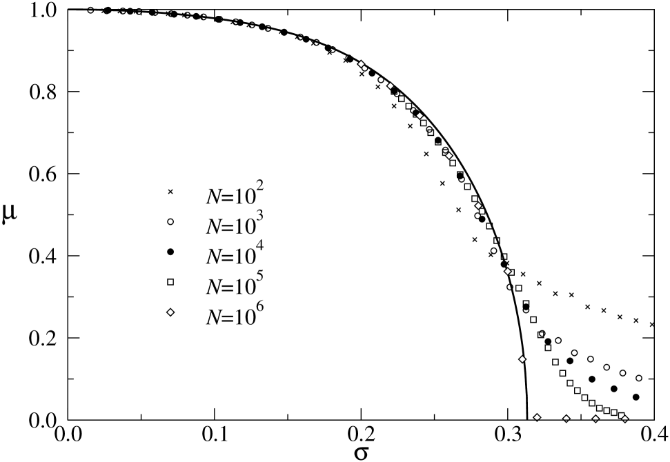
Figure 9: The order parameter $\mu$ as a function of the frequency dispersion $\sigma$, for ensembles of various sizes $N$. The curve corresponds to the analytical evaluation of $\mu$, from Eq. (21).

Taking into account that, in the limit $\sigma\to 0$, the relation (14) is equivalent to the stationarity condition for an ensemble with homogeneous phase distribution, for larger values of $\sigma$ we can write

$$\phi_{i}=\pm(\theta_{i}-\delta_{i})+\phi_{0},$$ (17)

where $\delta_{i}(t)$ measures the deviation of each oscillator with respect to the stationary state of small frequency dispersion. We assume that, for sufficiently large ensembles and long times, the distribution of these deviations is given by a well-defined function $p(\delta)$, satisfying $p(\delta)=p(-\delta)$. Implicitly, this also amounts to conjecture that the values of $\delta_{i}$ on the one hand, and $\phi_{i}$ and $\theta_{i}$ on the other, are not correlated. Replacing Eq. (17) into the definition of ${\bf m}_{i}$ and using Eq. (16) to calculate the order parameter $\mu$, we find

$$\mu=\int_{-\pi}^{\pi}p(\delta)\cos\delta d\delta.$$ (18)

Assuming that $\phi_{0}$ in Eq. (17) is independent of time, Eqs. (13) and (18) yield the following evolution equation for $\delta_{i}$:

$$\dot{\delta}_{i}=\Omega_{i}-\frac{\mu}{2}\sin\delta_{i}.$$ (19)

This equation has been extensively discussed in connection with the dynamics of globally coupled phase oscillators [21]. For $|\Omega_{i}|<\mu/2$, $\delta_{i}$ has two fixed points, at the solutions of

$$\sin\delta_{i}=\frac{2\Omega_{i}}{\mu}.$$ (20)

One of them is stable, and the other is unstable. On the other hand, for $|\Omega_{i}|>\mu/2$, there are no stable fixed points and $|\delta_{i}|$ grows indefinitely with time. We can therefore distinguish between two subpopulations in the ensemble, with qualitatively different behaviour. Those oscillators for which $|\Omega_{i}|<\mu/2$ reach, at asymptotically large times, a stationary deviation $\delta_{i}$. In contrast, for those oscillator with $|\Omega_{i}|>\mu/2$ the phase $\phi_{i}$ does not reach a stationary value with respect to the internal variable $\theta_{i}$. We refer to these two subpopulations as subensembles I and II, respectively. Whether a given oscillator belongs to one of the two subensembles depends on the value of $\mu$. According to Eq. (18), $\mu$ is given by the distribution of stationary deviations $\delta_{i}$, which in turn depend on $\mu$ through Eq. (20). Thus, the order parameter must be found self-consistently.

The distribution of deviations $p(\delta)$ consists of contributions from each subensemble $p=p_{\rm I}+p_{\rm II}$. Since the deviations $\delta_{i}$ for the oscillators of subensemble II are not stationary and move at different velocities, $p_{\rm II}(\delta)$ is a flat distribution and, thus, does not contribute to $\mu$ in Eq. (18). The contribution of subensemble I, on the other hand, can be found from the identity $p_{\rm I}(\delta)d\delta=g(\Omega)d\Omega$, taking into account the connection between the deviation and the internal frequency of each oscillator, given through $\mu$ by Eq. (20). Replacing $p(\delta)$ into Eq. (18) yields

$$\mu=\int_{-\mu/2}^{\mu/2}g(\Omega)\sqrt{1-\frac{4\Omega^{2}}{\mu^{2}}}d\Omega.$$ (21)

This is the self-consistency equation which makes it possible to find $\mu$, given the distribution of internal frequencies $g(\Omega)$. For our Gaussian distribution, Eq. (21) has a nontrivial solution $\mu>0$ if $\sigma<\sigma_{c}=\sqrt{\pi/32}\approx 0.313$. As the frequency dispersion approaches the critical value $\sigma_{c}$ from below, the order parameter vanishes as $\mu\sim|\sigma-\sigma_{c}|^{1/2}$. For $\sigma>\sigma_{c}$, the only solution is $\mu=0$. The curve in Fig. 9 shows the solution to Eq. (21) as a function of the frequency dispersion. The excellent agreement with numerical results validate our analytical approach. Remnant discrepancies can be ascribed to the enhancement of finite-size effects around the critical transition.

Note that the same singular dependence of the order parameter $\mu$ close to the order-disorder transition would be found for a broad class of frequency distributions $g(\Omega)$. In fact, since only small values of $\Omega$ contribute to the integral in Eq. (21) when $\mu$ is small, the critical behaviour is determined by the shape of the maximum of $g(\Omega)$ at $\Omega=0$. Suppose that, for $\Omega\approx 0$, we have $g(\Omega)\approx g(0)-\gamma\Omega^{2}$. Replacing into Eq. (21) we find

$$\mu=8\sqrt{\frac{1}{\pi\gamma}\left[1-\frac{\pi}{4}g(0)\right]}.$$ (22)

Consequently, the critical point is determined by the equation $g(0)=4/\pi$. If, sufficiently close to the point where this equation holds, $g(0)$ varies linearly with the control parameter $\sigma$, the order parameter will behave as $\mu\sim|\sigma-\sigma_{c}|^{1/2}$. The critical exponent, here equal to $1/2$, changes if the maximum of $g(\Omega)$ at $\Omega=0$ is not quadratic.

Using the complex vector $\bf m$ defined in Eq. (16), the equation of motion (13) for the phase of an individual oscillator can be recast as

$$\dot{\phi}_{i}=\frac{\mu_{+}}{2}\sin(\psi_{+}+\theta_{i}-\phi_{i})+\frac{\mu_{-}}{2}\sin(\psi_{-}-\theta_{i}-\phi_{i}).$$ (23)

The form of this equation emphasizes the mean-field nature of the interactions, as $\dot{\phi}_{i}$ depends only on the individual variables $\phi_{i}$ and $\theta_{i}$ and on the averages involved in the definition of $\bf m$. Since for asymptotically large ensembles, $N\to\infty$, $\mu=\sqrt{\mu_{+}^{2}+\mu_{-}^{2}}$ is zero for $\sigma>\sigma_{c}$, both $\mu_{+}$ and $\mu_{-}$ must also vanish beyond the transition. This implies that in the thermodynamical limit and for $\sigma>\sigma_{c}$, $\dot{\phi}_{i}=0$ and the dynamics is thus frozen. For finite systems, $\mu_{+}$ and $\mu_{-}$ are of order $N^{-1/2}$. The evolution of individual phases can therefore be thought as driven by random forces of that order. Below the transition, evolution becomes progressively slower as $\sigma$ approaches the critical point.

3.3 Dynamical clustering

As pointed out above, the dynamical regimes of small and large frequency dispersion are separated by a region, around $\sigma\approx 0.3$, where clustering is found (Fig. 8b). To disclose the properties of this intermediate regime, we have numerically studied the evolution of the distribution of phases $\phi_{i}$. Recording the evolution of each phase, we construct a histogram where the height of the column with base $(\phi,\phi+\Delta\phi)$ is proportional to the number of oscillators whose phases lie within that interval. Figure 10 shows a density plot of such histogram as a function of time, for $\sigma=0.3$.

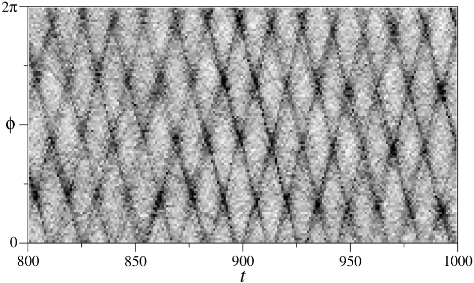
Figure 10: Density plot of the phase distribution ($100$-column histogram) as a function of time, for a system of $N=10^{3}$ oscillators with frequency dispersion $\sigma=0.3$, along $200$ time units. Darker tones correspond to higher concentrations.

We note that a fraction of the ensemble is entrained into four clusters. A close inspection of these clusters shows that they are formed by the oscillators of subensemble II (see Sect. 3.2) with internal frequencies just above their lowest value, $|\Omega_{i}|\gtrsim\mu/2$. Though the clusters are not sharply localized, it is still possible to define their phase by averaging $\phi_{i}$ over the oscillators belonging to each cluster. Two of these clusters, whose phases differ by $\pi$, move at a well defined velocity in one direction. The other two, whose phases also differ by $\pi$, move in the opposite direction and with the same speed. The two pairs of clusters are formed by oscillators whose internal frequencies have opposite signs. Figure 11a illustrates the situation. Due to their contrary motion, the two pairs of clusters cross each other recurrently. When these crossings happen, their populations are temporarily superimposed in phase. Consequently, two big clusters with opposite phases are recurrently built up (Figs. 10 and 11b). Figure 8b shows a $100$-oscillator ensemble at one of such events.

The recursive formation of the two anti-phase big clusters can be quantitatively characterized by an order parameter. The modulus of the complex quantity

$$z(t)=\frac{1}{N}\sum_{i}\exp(2{\rm i}\phi_{i})$$ (24)

is approximately equal to one if the whole ensemble splits into two anti-phase well-localized clusters of similar sizes, while for incoherent or higher-order clustered states we have $|z|\sim N^{-1/2}$. Figure 12a shows the evolution of $|z(t)|$ in the clustering regime, displaying its irregular oscillations between small and large values. For the same realization, Fig. 12b shows the phase difference $\Delta\phi=\phi_{a}-\phi_{b}$ for two oscillators $a$ and $b$ in subensemble II. Large positive values of $\cos\Delta\phi$ identify states where the two oscillators are part of the same cluster, while negative values correspond to the situation where they are in different clusters. The intermittent transitions of $\cos\Delta\phi$ between positive and negative values demonstrate the dynamical nature of clustering, where clusters maintain their identity but elements can migrate between them.

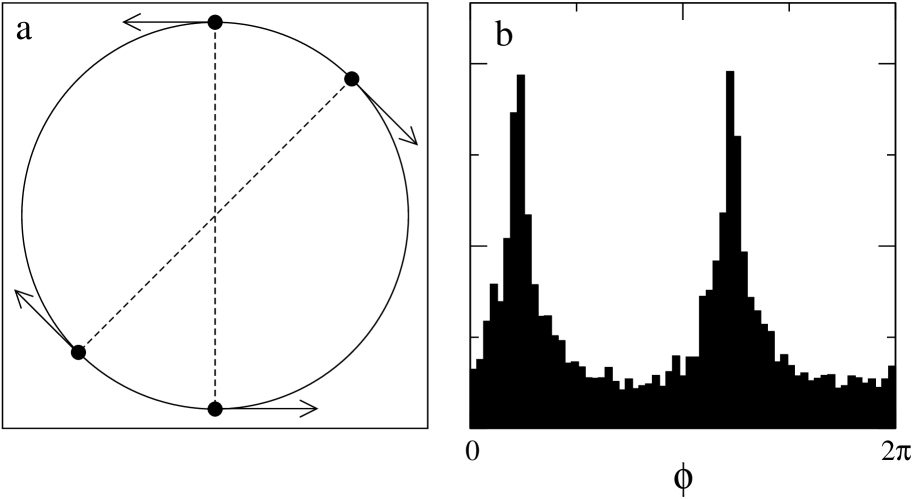
Figure 11: (a) Schematic representation of the relative position and motion of the two pair of clusters found in the clustering regime. (b) Histogram of the distribution of phases when the two cluster pairs cross each other, in a system of $N=10^{3}$ oscillators with frequency dispersion $\sigma=0.3$.

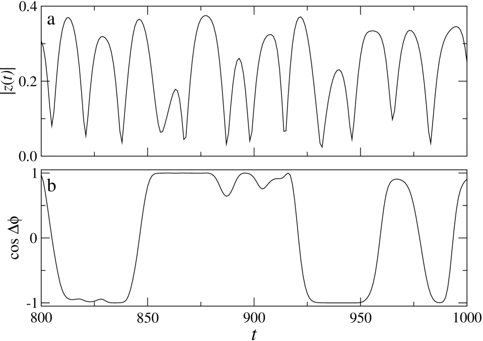
Figure 12: (a) Evolution of $|z(t)|$, Eq. (24), for a system of $N=10^{3}$ oscillators wit h frequency dispersion $\sigma=0.3$. (b) Phase difference of two oscillators of subensemble II with similar frequencies, in the same realization as in (a).

The average of $|z(t)|$ over long times provides a suitable order parameter, $\zeta$, for the detection of clustered states. Note that $\zeta$ and $\mu$ are independent order parameters, as they measure Fourier contributions of different order to the distribution of phases. Figure 13 shows numerical results for $\zeta$ as a function of the frequency dispersion. As $\sigma$ approaches the critical value $\sigma_{c}$ from below, $\zeta$ grows and exhibits a peak just at the left of the critical point. The profile of this peak becomes better defined as the ensemble size $N$ grows. The order parameter grows from zero at $\sigma\approx 0.2$ and reaches the maximum value $\zeta\approx 0.25$ for $\sigma\lesssim\sigma_{c}$. Beyond the transition, $\zeta$ drops abruptly. Results for the largest ensembles suggest that, in the thermodynamical limit, it vanishes for $\sigma>\sigma_{c}$. The suppression of clustering beyond the transition is a consequence of the fact that, as discussed in Sect. 3.2, the evolution of asymptotically large ensembles becomes frozen. As $\sigma$ approaches the critical point and the order parameter $\mu$ tends to vanish, the typical evolution time scales –which, according to Eq. (23), are of order $\mu^{-1}$– are increasingly large. Thus, the formation of clusters is progressively retarded and, finally, it is suppressed.

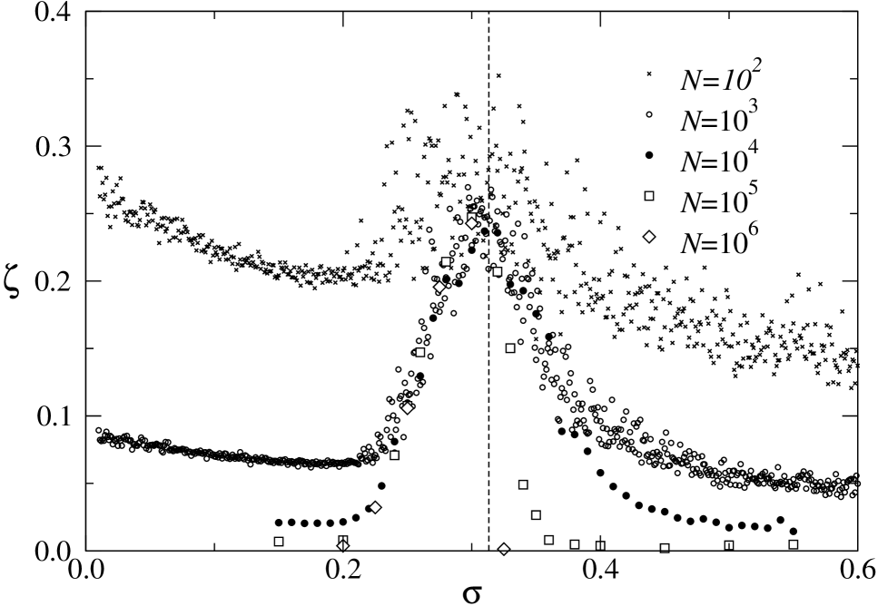
Figure 13: The order parameter $\zeta$ as a function of the frequency dispersion $\sigma$ for oscillator ensembles of various sizes. The vertical dashed line indicates the critical point of the order-disorder transition, $\sigma_{c}=\sqrt{\pi/32}$.

The appearance of the four clusters in the transition regime can be qualitatively understood taking into account that, for an oscillator with internal frequency $\Omega_{i}$, the most persistent interactions affecting its dynamics are due to oscillators with similar frequencies, $\Omega_{j}\approx\Omega_{i}$. In such case, in fact, the interaction weight $V(\theta_{i},\theta_{j})$ remains almost constant over very long time scales, of order $|\Omega_{i}-\Omega_{j}|^{-1}$. Fixing the attention on a group of oscillators with similar frequencies, we realize that their interactions are weighted by almost time-independent factors which, however, can take a different value for each oscillator pair. We can have both positive and negative interaction weights. Now, it is known that an ensemble of coupled oscillators with disordered interactions forms, if the level of frustration is moderate, two anti-phase localized clusters [18]. In our system, triggering the formation of these two clusters requires moreover that the phases $\phi_{i}$ are not pinned to the internal variables $\theta_{i}$, and that a sufficiently large population with similar frequencies actually exist. These two conditions are met by the oscillators of subensemble II with frequencies close to the limit $|\Omega|=\mu/2$, where the density is larger. We expect that two clusters form in the region of positive frequencies, and other two clusters appear for $\Omega<0$. The symmetry of this configuration insures that the two pairs of clusters will move in opposite direction and with the same speed. As far as $\sigma$ remains below the transition point, increasing the frequency dispersion contributes in two cooperating ways to the growth of the population of these clusters: larger values of $\sigma$ imply more oscillators with higher internal frequencies and, at the same time, a larger fraction in subensemble II, as $\mu$ decreases.

4 Conclusion

We have studied, both numerically and analytically, the dynamical regimes of an ensemble of coupled motile elements whose interactions are determined by the evolution of their internal states. The interaction of each pair of elements is alternatively attractive or repulsive, changing its sign within time scales associated with the relative variation of the respective internal variables. Though in our study we have considered specific forms both for the spatial dependence of the interactions and for their modulation by the internal state, our main results are expected to hold for a broad class of similar models. The following summary is focused on such generic conclusions.

Transitions between different dynamical regimes are controlled by two parameters: the range of interactions and the typical evolution time of the internal variables. The latter determines, in turn, the time scales within which interactions change their sign. The simultaneous presence of both positive and negative pair interactions induces the formation of localized clusters of mutually attracting elements. The remnant repulsion drives clusters away from each other, a tendency to expansion that must be counteracted by suitable boundary conditions. Due to the change of the sign of interactions, clustering is dynamical, as elements intermittently aggregate, disperse, and migrate between clusters. The actual development of localized clusters, however, requires that the interaction range is neither too small nor too large. Clusters are practically not formed if that range is smaller than the average distance between elements, while for large interaction ranges other kinds of spatial organization, such as “strings” of elements and condensation in the boundaries, become more frequent.

When the range of interactions is large as compared with the spatial size of the system, interactions act in conditions similar to those of global coupling [17], though different interaction weights are still possible between different element pairs. In such conditions, the spatial distribution of the ensemble becomes less relevant to the collective dynamics, because interactions are now independent of the relative position of elements. Yet, their individual positions are still determined by their interactions, which are now mainly driven by the internal variables. When the evolution of the internal variables is sufficiently slow, the spatial distribution can follow it almost adiabatically, and the relative position of the elements adjusts to their instantaneous internal state. As a result, a state of high correlation between spatial and internal variables develops. Due to the autonomous internal evolution of each element, this ordered state is dynamical, and the spatial distribution keeps varying with time. On the other hand, if the internal variables change too fast, the spatial coordinates fail to follow their evolution, and correlation between them breaks down. If the internal evolution is sufficiently fast and the time average of pair interactions is zero, the spatial distribution of the ensemble becomes frozen. In our specific model, the transition between the ordered and the disordered state has the properties of a critical phenomenon. In the disordered state, evolution is frozen in the limit of an infinitely large ensemble. The transition is mediated by a regime of dynamical clustering, induced by the persistent interaction between elements whose internal variables change within similar time scales, and whose positions and internal states are not strongly correlated.

The dynamics of internal states is expected to be an essential ingredient in the description of systems whose collective evolution resembles the complex collective dynamics of biological and social populations [14]. Spontaneous development of coherent behaviour may be enhanced if individual internal variables are allowed to interact with each other. In fact, the organization of the ensemble at the level of the individual internal states, due to their mutual interaction, would imply coherence also at the level of other variables, such as the spatial position. These processes are expected to be relevant to the modeling of social-like mechanisms, of the type of imitation, social influence, and formation of coalitions and hierarchical structures. The investigation of their role in the emergence of order has already been initiated in the literature [15], also in connection with evolutionary adaptive phenomena [22, 23, 24].

References

- [1] A. S. Mikhailov and V. Calenbuhr, From Cells to Societies. Models of Complex Coherent Action, Springer, Berlin, 2002.
- [2] A. Pikovsky, M. Rosemblum and J. Kurths, Synchronization. A Universal Concept in Nonlinear Sciences, Cambridge University Press, 2001.
- [3] J. Buck and E. Buck, Synchronous fireflies, Sci. Am. 234 (1976) 74.
- [4] E. Sismondo, Synchronous, alternating, and phase-locked stridulation by a tropical katydid, Science 249 (1990) 55.
- [5] K. Kaneko, Clustering, coding, switching, hierarchical ordering, and control in a network of chaotic elements, Physica D 41 (1990) 137.
- [6] D. H. Zanette and A. S. Mikhailov, Condensation in globally coupled populations of chaotic dynamical systems, Phys. Rev. E 57 (1998) 276.
- [7] D. H. Zanette and A. S. Mikhailov, Mutual synchronization of globally coupled neural networks, Phys. Rev. E 58 (1998) 872.
- [8] D. Golomb, D. Hansel, B. Shraiman and H. Sompolinsky, Clustering in globally coupled phase oscillators, Phys. Rev. A 45 (1992) 3516.
- [9] K. Okuda, Variety and generality of clustering in globally coupled oscillators, Physica D 63 (1993) 424.
- [10] D. Hansel, G. Mato and C. Meunier, Clustering and slow switching in globally coupled phase oscillators, Phys. Rev. E 48 (1993) 3470.
- [11] D. H. Zanette and A. S. Mikhailov, Dynamical clustering in large populations of Rössler oscillators under the action of noise, Phys. Rev. E 62 (2000) R7571.
- [12] H. Kori and Y. Kuramoto, Slow switching in globally coupled oscillators: robustness and occurrence through delayed coupling, Phys. Rev. E 63 (2001) 046214.
- [13] P. Stange, D. H. Zanette, A. Mikhailov and B. Hess, Self-organizing molecular networks, Biophys. Chem. 72 (1998) 73.
- [14] R. Axelrod, The Complexity of Cooperation. Agent-Based Models of Competition and Collaboration, Princeton, Princeton University Press, 1997.
- [15] T. Shibata and K. Kaneko, Coupled map gas: structure formation and dynamics of interacting elements with internal dynamics, Physica D 181 (2003) 197.
- [16] A. T. Winfree, The Geometry of Biological Time, Springer, Berlin, 1980.
- [17] Y. Kuramoto, Chemical Oscillations, Waves, and Turbulence, Springer, Berlin, 1984.
- [18] H. Daido, Population dynamics of randomly interacting self-oscillators, Prog. Theor. Phys. 77 (1987) 622.
- [19] H. Daido, Quasientrainment and slow relaxation in a population of oscillators with random and frustrated interactions, Phys. Rev. Lett. 68 (1992) 1073.
- [20] H. Daido, Algebraic relaxation of an order parameter in randomply coupled limit-cycle oscillators, Phys. Rev. E 61 (2000) 2145.
- [21] H. Sakaguchi and Y. Kuramoto, A soluble active rotator model showing phase transitions via mutual entrainment, Prog. Theor. Phys. 76 (1986) 576.
- [22] P. Seliger, S. C. Young and L. S. Tsimring, Plasticity and learning in a network of coupled phase oscillators, Phys. Rev. E 65 (2002) 041906.
- [23] J. Ito and K. Kaneko, Spontaneous structure formation in a network of chaotic units with variable connection strengths, Phys. Rev. Lett. 88 (2002) 028701.
- [24] J. Ito and K. Kaneko, Spontaneous structure formation in a network of dynamical elements, Phys. Rev. E 67 (2003) 046226.