Excitons dressed by a sea of excitons

Abstract

We here consider an exciton $i$ embedded in a sea of $N$ identical excitons $0$. If the excitons are bosonized, a bosonic enhancement factor, proportional to $N$, is found for $i=0$. If the exciton composite nature is kept, this enhancement not only exists for $i=0$, but also for any exciton having a center of mass momentum equal to the sea exciton momentum. This physically comes from the fact that an exciton with such a momentum can be transformed into a sea exciton by “Pauli scattering”, i. e., carrier exchange with the sea, making this $i$ exciton not so much different from a $0$ exciton. This possible scattering, directly linked to the composite nature of the excitons, is irretrievably lost when the excitons are bosonized.

This work in fact deals with the quite tricky scalar products of $N$-exciton states. It actually constitutes a crucial piece of our new many-body theory for interacting composite bosons, because all physical effects involving these composite bosons ultimately end by calculating such scalar products. The “Pauli diagrams” we here introduce to represent them, allow to visualize many-body effects linked to carrier exchange in an easy way. They are conceptually different from Feynman diagrams, because of the special feature of the “Pauli scatterings”: These scatterings, which originate from the departure from boson statistics, do not have their equivalent in Feynman diagrams, the commutation rules for exact bosons (or fermions) being included in the first line of the usual many-body theories.

PACS.: 71.35.-y Excitons and related phenomena

1 Introduction

We are presently developing a new many-body theory [1-7] able to handle interactions between composite bosons — like the semiconductor excitons. The development of such a theory is in fact highly desirable, because, in the low density limit, electron-hole pairs are known to form bound excitons, so that, in this limit, to manipulate excitons is surely a better idea than to manipulate free carriers. However, the interaction between excitons is not an easy concept due to carrier indistinguishability: Indeed, the excitons, being made of two charged particles, of course interact through Coulomb interactions. However, this Coulomb interaction can be $(V_{ee^{\prime}}+V_{hh^{\prime}}-V_{eh^{\prime}}-V_{e^{\prime}h})$ or $(V_{ee^{\prime}}+V_{hh^{\prime}}-V_{eh}-V_{e^{\prime}h^{\prime}})$ depending if we see the excitons as $(e,h)$ and $(e^{\prime},h^{\prime})$, or $(e,h^{\prime})$ and $(e^{\prime},h)$. In addition, excitons interact in a far more subtle manner through Pauli exclusion between their indistinguishable components, in the absence of any Coulomb process. This “Pauli interaction” is actually the novel and interesting part of our new many-body theory for composite bosons. It basically comes from the departure from boson statistics, all previous theories, designed for true bosons or true fermions, having the corresponding commutation rules set up in the first line [8]. In our theory, the fact that the excitons are not exact bosons appears through “Pauli scatterings” $\lambda_{mnij}$ between the “in” excitons $(i,j)$ and the “out” excitons $(m,n)$. Their link to boson departure is obvious from their definition. Indeed, these Pauli scatterings appear through [2,3]

$$[B_{m},B_{i}^{\dagger}]=\delta_{mi}-D_{mi}\ ,$$ (1)

$$[D_{mi},B_{j}^{\dagger}]=2\sum_{n}\lambda_{mnij}\,B_{n}^{\dagger}\ ,$$ (2)

$B_{i}^{\dagger}$ being the $i$ exciton creation operator. It precisely reads in terms of the exciton wave function $\phi_{i}(\mathbf{r}_{e},\mathbf{r}_{h})=\langle\mathbf{r}_{e},\mathbf{r}_{h}|B_{i}^{\dagger}|v\rangle$ as

$$\lambda_{mnij}=\frac{1}{2}\int d\mathbf{r}_{e}\,d\mathbf{r}_{e^{\prime}}\,d\mathbf{r}_{h}\,d\mathbf{r}_{h^{\prime}}\,\phi_{m}^{\ast}(\mathbf{r}_{e},\mathbf{r}_{h})\,\phi_{n}^{\ast}(\mathbf{r}_{e^{\prime}},\mathbf{r}_{h^{\prime}})\,\phi_{i}(\mathbf{r}_{e},\mathbf{r}_{h^{\prime}})\,\phi_{j}(\mathbf{r}_{e^{\prime}},\mathbf{r}_{h})\ +\ (m\leftrightarrow n)\ .$$ (3)

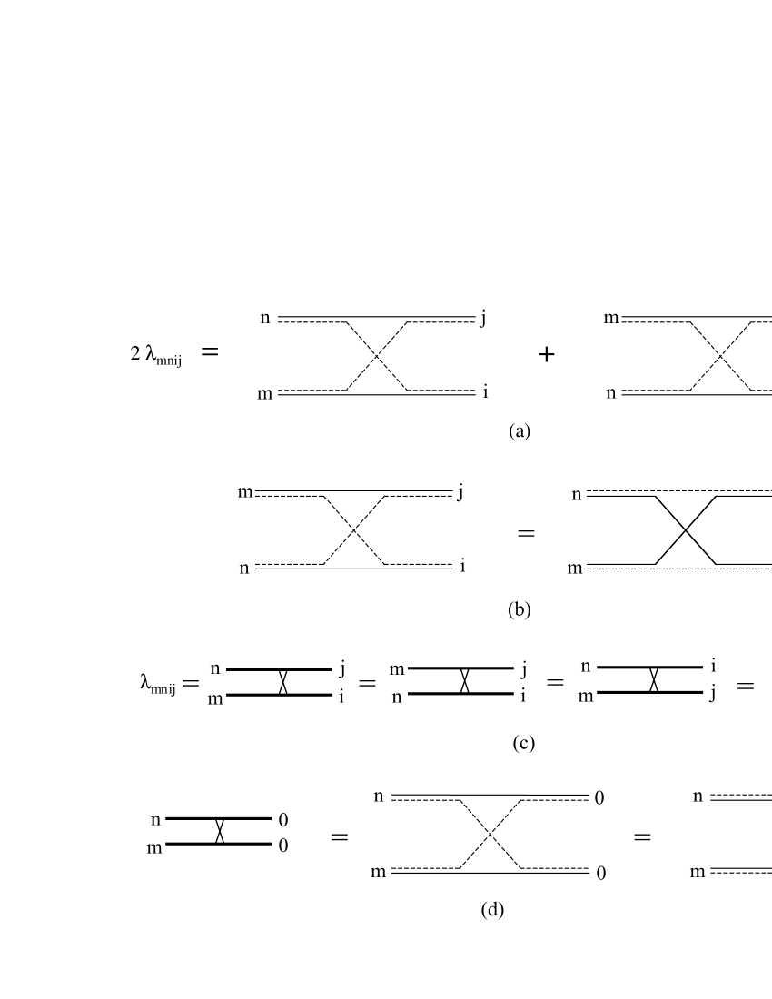
Figure 1: Pauli scattering $\lambda_{mnij}$ between the “in” excitons $(i,j)$ and the “out” excitons $(m,n)$. Solid line: electron; dashed line: hole; heavy solid line: exciton. (a): As defined in eq. (3), $\lambda_{mnij}$ is composed of two hole exchanges, with the exciton indices $(m,n)$ inverted, so that $\lambda_{mnij}=\lambda_{nmij}=\lambda_{mnji}$. (b): A hole exchange between $(i,j)$ and $(n,m)$ corresponds to an electron exchange between $(i,j)$ and $(m,n)$. (c): In the Pauli diagrams of the following figures, the Pauli scatterings $\lambda_{mnij}$ will be represented by crosses. (d) and (e): When the two indices on one side are equal, the two processes of $\lambda_{mnij}$ are identical: $\lambda_{mnij}$ either corresponds to a hole exchange as in (d) or an electron exchange as in (e).

The above expression makes clear the fact that $\lambda_{mnij}$ just corresponds to a carrier exchange between two excitons (see fig. 1a) without any Coulomb process, so that $\lambda_{mnij}$ is actually a dimensionless “scattering”. It is possible to show that for bound states, $\lambda_{mnij}$ is of the order of $\mathcal{V}_{X}/\mathcal{V}$, with $\mathcal{V}_{X}$ being the exciton volume and $\mathcal{V}$ the sample volume [6].

All physical quantities involving excitons can be written as matrix elements of an Hamiltonian dependent operator $f(H)$ between $N$-exciton states, with usually most of them in the ground state $0$. These matrix elements formally read

$$\langle v|B_{m_{1}}\cdots B_{m_{n}}B_{0}^{N-n}\,f(H)\,B_{0}^{{\dagger}N-n^{\prime}}B_{i_{1}}^{\dagger}\cdots B_{i_{n^{\prime}}}^{\dagger}|v\rangle\ .$$ (4)

They can be calculated by “pushing” $f(H)$ to the right in order to end with $f(H)|v\rangle$, which is just $f(0)|v\rangle$ if the vacuum is taken as the energy origin. This push is done through a set of commutations. In the simplest case, $f(H)=H$, we have

$$HB_{i}^{\dagger}=B_{i}^{\dagger}(H+E_{i})+V_{i}^{\dagger}\ ,$$ (5)

which just results from [2,3]

$$[H,B_{i}^{\dagger}]=E_{i}B_{i}^{\dagger}+V_{i}^{\dagger}\ .$$ (6)

We then push $V_{i}^{\dagger}$ to the right according to

$$[V_{i}^{\dagger},B_{j}^{\dagger}]=\sum_{mn}\xi_{mnij}^{\mathrm{dir}}\,B_{m}^{\dagger}B_{n}^{\dagger}\ ,$$ (7)

to end with $V_{i}^{\dagger}|v\rangle$ which is just $0$ due to eq. (6) applied to $|v\rangle$.

Equations (6,7), along with eqs. (1,2), form the four key equations of our many-body theory for interacting composite excitons. $\xi_{mnij}^{\mathrm{dir}}$ is the second scattering of this theory. It transforms the $(i,j)$ excitons into $(m,n)$ states, due to Coulomb processes between them, as obvious from its explicit expression:

$$\xi_{mnij}^{\mathrm{dir}}=\frac{1}{2}\int d\mathbf{r}_{e}\,d\mathbf{r}_{e^{\prime}}\,d\mathbf{r}_{h}\,d\mathbf{r}_{h^{\prime}}\,\phi_{m}^{\ast}(\mathbf{r}_{e},\mathbf{r}_{h})\,\phi_{n}^{\ast}(\mathbf{r}_{e^{\prime}},\mathbf{r}_{h^{\prime}})\hskip 113.81102pt$$

$$\times(V_{ee^{\prime}}+V_{hh^{\prime}}-V_{eh^{\prime}}-V_{e^{\prime}h})\,\phi_{i}(\mathbf{r}_{e},\mathbf{r}_{h})\,\phi_{j}(\mathbf{r}_{e^{\prime}},\mathbf{r}_{h^{\prime}})\ +(m\leftrightarrow n)\ .$$ (8)

Note that, in $\xi_{mnij}^{\mathrm{dir}}$, the “in” and “out” excitons are made with the same pairs, while, in $\lambda_{mnij}$, they have exchanged their carriers. Due to dimensional arguments, these $\xi_{mnij}^{\mathrm{dir}}$ for bound states are of the order of $R_{X}\mathcal{V}_{X}/\mathcal{V}$, with $R_{X}$ being the exciton Rydberg [6].

Another $f(H)$ of interest can be $1/(a-H)$, with $a$ possibly equal to $(\omega+i\eta)$ as in problems involving photons. In order to push $1/(a-H)$ to the right, we can use [4]

$$\frac{1}{a-H}\,B_{i}^{\dagger}=B_{i}^{\dagger}\,\frac{1}{a-H-E_{i}}+\frac{1}{a-H}\,V_{i}^{\dagger}\,\frac{1}{a-H-E_{i}}\ ,$$ (9)

which follows from eq. (5). In pushing $1/(a-H)$ to the right, we generate Coulomb terms through the $V_{i}^{\dagger}$ part of eq. (9). Due to dimensional arguments, these terms ultimately read as an expansion in $\xi_{mnij}^{\mathrm{dir}}$ over an energy denominator which can be either a detuning or just a difference between exciton energies, depending on the problem at hand.

A last $f(H)$ of interest is $e^{-iHt}$ which appears in problems involving time evolution. In order to push $e^{-iHt}$ to the right, we can use [7]

$$e^{-iHt}\,B_{i}^{\dagger}=B_{i}^{\dagger}\,e^{-i(H+E_{i})t}+W_{i}^{\dagger}(t)\ ,$$ (10)

$$W_{i}^{\dagger}(t)=-\int_{-\infty}^{+\infty}\frac{dx}{2i\pi}\,\frac{e^{-i(x+i\eta)t}}{x-H+i\eta}\,V_{i}^{\dagger}\,\frac{1}{x-H-E_{i}+i\eta}\ .$$ (11)

Equations (10,11) result from the integral representation of the exponential, namely

$$e^{-iHt}=-\int_{-\infty}^{+\infty}\frac{dx}{2i\pi}\,\frac{e^{-i(x+i\eta)t}}{x-H+i\eta}\ ,$$ (12)

valid for $t$ and $\eta$ positive, combined with eq. (9). Again additional Coulomb terms appear in passing $e^{-iHt}$ over $B_{i}^{\dagger}$.

By comparing eqs. (5,9,10), we see that, when we pass $f(H)$ over $B_{i}^{\dagger}$, we essentially replace it by $f(H+E_{i})$, as if the $i$ exciton was not interacting with the other excitons, within a Coulomb term which takes care of these interactions, $f(H+E_{i})$ being in some sense the zero order contribution of $f(H)$.

Once we have pushed all the $H$’s up to $|v\rangle$ and generated very many Coulomb scatterings $\xi_{mnij}^{\mathrm{dir}}$, we end with scalar products of $N$-exciton states which look like eq. (4) with $f(H)=1$. Then, we start to push the $B$’s to the right according to eqs. (1,2), to end with $B|v\rangle$ which is just zero. This set of pushes now makes appearing the Pauli scatterings $\lambda_{mnij}$.

In the case of $N=2$, eqs. (1,2) readily give the scalar product of two-exciton states as [2]

$$\langle v|B_{m}\,B_{n}\,B_{i}^{\dagger}\,B_{j}^{\dagger}|v\rangle=\delta_{mi}\,\delta_{nj}+\delta_{mj}\,\delta_{ni}-2\lambda_{mnij}\ .$$ (13)

For large $N$, the calculation of similar scalar products is actually very tricky. We expect them to depend on $N$ and to contain many $\lambda_{mnij}$’s.

The $N$ dependence of these scalar products is in fact crucial because physical quantities must ultimately depend on $\eta=N\mathcal{V}_{X}/\mathcal{V}$, with $\mathcal{V}_{X}/\mathcal{V}$ coming either from Pauli scatterings or from Coulomb scatterings — with possibly an additional factor $N$, if we look for something extensive. However, as the scalar products of $N$-exciton states are not physical quantities, they can very well contain superextensive terms in $N^{p}\eta^{n}$ which ultimately disappear from the final expressions of the physical quantities. To handle these factors $N$ properly — and their possible cancellations — is thus crucial.

In previous works [1,5], we have calculated the simplest of these scalar products of $N$-exciton states, namely $\langle v|B_{0}^{N}B_{0}^{{\dagger}N}|v\rangle$. We found it equal to $N!$, as for exact bosons, multiplied by a corrective factor $F_{N}$ which comes from the fact that excitons are composite bosons,

$$\langle v|B_{0}^{N}\,B_{0}^{{\dagger}N}|v\rangle=N!\,F_{N}\ .$$ (14)

This $F_{N}$ factor is actually superextensive, since it behaves as $e^{-N\,O(\eta)}$ (see ref. [5]). In large enough samples, $N\eta$ can be extremely large even for $\eta$ small, which makes $F_{N}$ exponentially small. In physical quantities however, $F_{N}$ never appears alone, but through ratios like $F_{N-p}/F_{N}$ which actually read as $1+O(\eta)$ for $p\ll N$. This restores the expected $\eta$ dependence of these physical quantities.

The present paper in fact deals with determining the interplay between the possible factors $N$ and the various $\lambda$’s which appear in scalar products of $N$-exciton states. These Pauli scatterings $\lambda$ being the original part of our many-body theory for interacting composite bosons, the understanding of this interplay is actually fundamental to master many-body effects between excitons at any order in $\eta=N\mathcal{V}_{X}/\mathcal{V}$. This will in particular allow us to cleanly show the cancellation of superextensive terms which can possibly appear in the intermediate stages of the theory [7].

This paper can appear as somewhat formal. It however constitutes one very important piece of this new many-body theory, because all physical effects between $N$ interacting excitons ultimately end with calculating such scalar products. Problems involving two excitons only[7] are in fact rather simple to solve because they only need the scalar product of two-exciton states given in eq. (13). The real challenging difficulty which actually remains in order to handle many-body effects between $N$ excitons at any order in $\eta$, is to produce the equivalent of eq. (13) for large $N$.

In usual many-body effects, Feynman diagrams [8] have been proved to be quite convenient to understand the physics of interacting fermions or bosons. We can expect the introduction of diagrams to be also quite convenient to understand the physics of interacting composite bosons. It is however clear that diagrams representing carrier exchange between $N$ excitons have to be conceptually new: In them, must enter the Pauli scatterings which take care of the departure from boson statistics. As the fermion or boson statistics is included in the first lines of the usual many-body theories, the Pauli scatterings do not have their equivalent in Feynman diagrams. Another important part of the present paper is thus to present these new “Pauli diagrams” and to derive some of their specific rules. As we will show, these Pauli diagrams are in fact rather tricky because they can look rather differently although they represent exactly the same quantity. To understand why these different diagrams are indeed equivalent, is actually crucial to master these Pauli diagrams. This is the subject of the last section of this paper. It goes through the introduction of “exchange skeletons” which are the basic quantities for carrier exchanges between more than two excitons. Their appearance is physically reasonable because Pauli exclusion is $N$-body “at once”, so that, when it plays a role, it in fact correlates all the carriers of the involved excitons through a unique process, even if this process can be decomposed into exchanges between two excitons only, as in the Pauli scatterings $\lambda_{mnij}$.

From a technical point of view, it is of course possible to calculate the scalar products of $N$-exciton states, just through blind algebra based on eqs. (1,2), and to get the right answer. However, in order to understand the appearance of the extra factors $N$ which go in front of the ones in $N\lambda\simeq N\mathcal{V}_{X}/\mathcal{V}=\eta$ and which are crucial to ultimately withdraw superextensive terms from physical quantities, it is in fact convenient to introduce the concept of “excitons dressed by a sea of excitons”, because these extra factors $N$ are physically linked to the underlying bosonic character of the excitons which is enhanced by the presence of an exciton sea. We will show that these extra factors $N$ are linked to the topology of the diagrammatic representation of these scalar products, which appears as “disconnected” when these extra $N$’s exist. This is after all not very astonishing because disconnected Feynman diagrams are known to also generate superextensive terms.

Let us introduce the exciton $i$ dressed by a sea of $N$ excitons $0$ as

$$|\psi_{i}^{(N)}\rangle=\frac{B_{0}^{N}B_{0}^{{\dagger}N}}{\langle v|B_{0}^{N}B_{0}^{{\dagger}N}|v\rangle}\ B_{i}^{\dagger}|v\rangle\ ,$$ (15)

The denominator $\langle v|B_{0}^{N}B_{0}^{{\dagger}N}|v\rangle$ is a normalization factor which makes the operator in front of $B_{i}^{\dagger}$ appearing as an identity in the absence of Pauli interactions with the exciton sea. Indeed, we can check that the vacuum state, dressed in the same way as

$$|\psi^{(N)}\rangle=\frac{B_{0}^{N}B_{0}^{{\dagger}N}}{\langle v|B_{0}^{N}B_{0}^{{\dagger}N}|v\rangle}\ |v\rangle\ ,$$ (16)

is just $|v\rangle$, as expected because no interaction can exist with the vacuum. On the opposite, subtle Pauli interactions take place between the exciton sea and an additional exciton $i$. As the dressed exciton $i$ contains one more $B^{\dagger}$ than the number of $B$’s, it is essentially a one-pair state. It can be written either in terms of free electrons and holes, or better in terms of one-exciton states. Since these states are the one-pair eigenstates of the semiconductor Hamiltonian $H$, they obey the closure relation $1=\sum_{m}B_{m}^{\dagger}|v\rangle\langle v|B_{m}$. So that $|\psi_{i}^{(N)}\rangle$ can be written as

$$|\psi_{i}^{(N)}\rangle=\sum_{m}A_{N}(m,i)\,B_{m}^{\dagger}|v\rangle\ ,$$ (17)

$$A_{N}(m,i)=\frac{\langle v|B_{m}\,B_{0}^{N}\,B_{0}^{{\dagger}N}\,B_{i}^{\dagger}|v\rangle}{\langle v|B_{0}^{N}\,B_{0}^{{\dagger}N}|v\rangle}\ .$$ (18)

This decomposition of $|\psi_{i}^{(N)}\rangle$ on one-exiton states makes appearing the scalar product of $(N+1)$-exciton states with $N$ of them in the exciton sea.

As the physics which controls the extra factors $N$ in these scalar products, is actually linked to the underlying bosonic character of the excitons, let us first consider boson-excitons in order to see how a sea of $N$ boson-excitons $0$ affects them.

2 Boson-excitons dressed by a sea of excitons

Instead of eq. (1), the commutation rule for boson-excitons is $[\bar{B}_{m},\bar{B}_{i}^{\dagger}]=\delta_{mi}$, so that the deviation-from-boson operator $D_{mi}$ for boson-excitons is zero, as the Pauli scatterings $\lambda_{mnij}$. From this boson commutator, we get by induction

$$[\bar{B}_{0}^{N},\bar{B}_{i}^{\dagger}]=\bar{B}_{0}^{N-1}[\bar{B}_{0},\bar{B}_{i}^{\dagger}]+[\bar{B}_{0}^{N-1},\bar{B}_{i}^{\dagger}]\bar{B}_{0}=N\delta_{0i}\,\bar{B}_{0}^{N-1}\ .$$ (19)

So that $\bar{B}_{0}^{N}\bar{B}_{0}^{{\dagger}N}|v\rangle=N!\,|v\rangle$, which shows that the normalization factor $F_{N}$ is just 1 for boson-excitons, while $|\bar{\psi}_{0}^{(N)}\rangle=(N+1)\bar{B}_{0}^{\dagger}|v\rangle$ and $|\bar{\psi}_{i\neq 0}^{(N)}\rangle=\bar{B}_{i}^{\dagger}|v\rangle$. So that, we do have

$$|\bar{\psi}_{i}^{(N)}\rangle=(N\delta_{i0}+1)\,\bar{B}_{i}^{\dagger}|v\rangle\ .$$ (20)

The factor $N$ which appears in this equation is physically linked to the well known bosonic enhancemen [9]. The memory of such an effect must a priori exist for composite bosons, such as the excitons. However, subtle changes are expected due to their underlying fermionic character. Let us now see how this bosonic enhancement, obvious for boson-excitons, does appear for exact excitons.

3 Exact excitons dressed by a sea of excitons

The commutation rule for exact excitons is given in eq. (1). By taking another commutation, we generate eq. (2) which defines the Pauli scattering $\lambda_{mnij}$. From it, we easily get by induction

$$[D_{mi},B_{0}^{{\dagger}N}]=2N\sum_{n}\lambda_{mn0i}\,B_{n}^{\dagger}B_{0}^{{\dagger}N-1}\ ,$$ (21)

its conjugate leading to

$$[B_{0}^{N},D_{mi}]=2N\sum_{j}\lambda_{m0ji}\,B_{0}^{N-1}B_{j}\ ,$$ (22)

since $D_{mi}^{\dagger}=D_{im}$, while $\lambda_{mnij}^{\ast}=\lambda_{ijmn}$. Equation (21) allows to generalize eq. (1) as

$$[B_{m},B_{0}^{{\dagger}N}]=NB_{0}^{{\dagger}N-1}(\delta_{m0}-D_{m0})-N(N-1)\sum_{n}\lambda_{mn00}B_{n}^{\dagger}B_{0}^{{\dagger}N-2}\ ,$$ (23)

its conjugate leading to

$$[B_{0}^{N},B_{i}^{\dagger}]=N(\delta_{0i}-D_{0i})B_{0}^{N-1}-N(N-1)\sum_{j}\lambda_{00ij}B_{j}B_{0}^{N-2}\ .$$ (24)

(We can note that eq. (19) for bosons just follows from eq. (24), since the deviation-from-boson operator $D_{mi}$ and the Pauli scattering $\lambda_{mnij}$ are equal to zero in the case of boson-excitons).

In order to grasp the bosonic enhancement for exact excitons, let us start with the “best case” for such an enhancement, namely an exciton $0$ dressed by a sea of $N$ excitons $0$.

3.1 Exciton $0$ dressed by $N$ excitons $0$

According to eq. (17), this dressed exciton can be writen as

$$|\psi_{0}^{(N)}\rangle=(N+1)\sum_{m}\zeta_{N}(m)B_{m}^{\dagger}|v\rangle\,$$ (25)

in which we have set

$$\zeta_{N}(m)=\frac{A_{N}(m,0)}{N+1}=\frac{\langle v|B_{0}^{N}B_{m}B_{0}^{{\dagger}N+1}|v\rangle}{(N+1)!F_{N}}\ .$$ (26)

This $\zeta_{N}(m)$, which is just $F_{N+1}/F_{N}\simeq 1+O(\eta)$ for $m=0$, will appear to be a quite useful quantity in the following. To calculate it, we rewrite $B_{m}B_{0}^{{\dagger}N+1}$ according to eq. (23). Since $D_{m0}|v\rangle=0$, which follows from eq. (1) applied to $|v\rangle$, this readily gives the recursion relation between the $\zeta_{N}(m)$’s as

$$\zeta_{N}(m)=\delta_{m0}-\frac{F_{N-1}}{F_{N}}\,N\sum_{n}\lambda_{mn00}\,\zeta_{N-1}^{\ast}(n)\ .$$ (27)

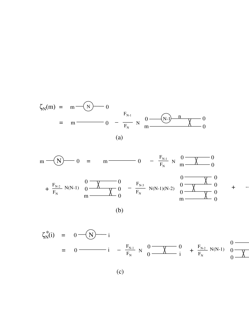
Figure 2: (a): Recursion relation for the matrix element $\zeta_{N}(m)$ defined in eq. (26). The $(m,0)$ line represents $\delta_{m0}$, while the cross represents the Pauli scattering $\lambda_{mn00}$ (see fig. 1). Sum is taken over the intermediate $n$ exciton. (b): Pauli diagrams for $\zeta_{N}(m)$ obtained by iteration of fig. 2a. They allow to visualize eq. (28) in a simple way. Sums are taken over the (unlabelled) exciton lines. (c): The complex conjugate of $\zeta_{N}(i)$ is represented by similar zigzag diagrams; the relative position of the crosses are just changed, being alternatively left, right, left,…, instead of right, left, right,…as in (b).

Its diagrammatic representation is shown in fig. 2a as well as its iteration (fig. 2b). Its solution is

$$\zeta_{N}(m)=\sum_{p=0}^{N}(-1)^{p}\frac{F_{N-p}}{F_{N}}\,\frac{N!}{(N-p)!}\,z^{(p)}(m,0)\ ,$$ (28)

with $z^{(0)}(m,0)=\delta_{m0}$, while

$$z^{(p)}(m,0)=\sum_{n}\lambda_{mn00}\,\left[z^{(p-1)}(n,0)\right]^{\ast}\ .$$ (29)

$z^{(p)}(m,0)$ can be represented by a diagram with $(p+1)$ lines, the lowest one being $(m,0)$, while the $p$ other lines are $(0,0)$. These lines are connected by $p$ Pauli scatterings which are in zigzag, alternatively right, left, right…(see fig. 2b). For $p=1$, $z^{(p)}(m,0)$ is just $\lambda_{m000}$, while for $p=2$, it reads $\sum_{n}\lambda_{mn00}\lambda_{00n0}$ and so on …Fig. 2c also shows $\zeta_{N}^{\ast}(i)$, easy to obtain from $\zeta_{N}(m)$ by noting that $\lambda_{mnij}^{\ast}=\lambda_{ijmn}$, so that $\zeta_{N}^{\ast}(i)$ is just obtained from $\zeta_{N}(i)$ by a symmetry right-left: In $\zeta_{N}^{\ast}(i)$, the zigzag in fact appears as left, right, left,…

Since we are ultimately interested in possible extra factors $N$, it can be of interest to understand the appearance of $N$’s in $\zeta_{N}(m)$. If we forget about the composite nature of the exciton, i. e., if we drop all carrier exchanges with the exciton sea, the electron and hole of the exciton $0$ are tight for ever as for boson-excitons, so that we should have for $|\psi_{0}^{(N)}\rangle$ the same result as the one for boson-excitons, namely $|\psi_{0}^{(N)}\rangle\simeq(N+1)B_{0}^{\dagger}|v\rangle$. This leads to $\zeta_{N}(m)\simeq\delta_{m0}$ at lowest order in $\lambda$. The composite exciton $0$ can however exchange its electron or its hole with one sea exciton to become an $m$ exciton. Since there are $N$ possible excitons in the sea for such an exchange, the first order term in exchange scattering must appear with a factor $N$. Another exciton, among the $(N-1)$ left in the sea, can also participate to these carrier exchanges so that the second order term in Pauli scattering must appear with a $N(N-1)$ prefactor; and so on …

From this iteration, we thus conclude that $\zeta_{N}(m)$ contains the same number of factors $N$ as the number of $\lambda$’s. Since, for $0$ and $m$ being bound states, these $\lambda$’s are in $\mathcal{V}_{X}/\mathcal{V}$, while $F_{N-p}/F_{N}$ reads as an expansion in $\eta$ (see ref. [5]), we thus find that, in the large $N$ limit, $\zeta_{N}(m)$ can be written as an expansion in $\eta$, without any extra factor $N$ in front. This thus shows that $|\psi_{0}^{(N)}\rangle$ contains the same bosonic enhancement factor $(N+1)$ as the one of dressed boson-excitons $|\bar{\psi}_{0}^{(N)}\rangle$. Let us however stress that the relative weight of the $B_{0}^{\dagger}|v\rangle$ state in $|\psi_{0}^{(N)}\rangle$, namely $\zeta_{N}(0)$, which is exactly 1 in the case of boson-excitons, is somewhat smaller than 1 due to possible carrier exchanges with the exciton sea. From the iteration of $\zeta_{N}(0)$, we find that this weight reads $\zeta_{N}(0)=1-(F_{N-1}/F_{N})N\lambda_{0000}+\cdots$, which is nothing but $F_{N+1}/F_{N}$ as can be directly seen from eq. (26).

To compensate this decrease of the $B_{0}^{\dagger}|v\rangle$ state weight, $|\psi_{0}^{(N)}\rangle$ has non-zero components on the other exciton states $B_{m\neq 0}^{\dagger}|v\rangle$, in contrast with the boson-exciton case. We can however note that, since $\zeta_{N}(m)=0$ for $\mathbf{Q}_{m}\neq\mathbf{Q}_{0}$, due to momentum conservation in Pauli scatterings, the other exciton states making $|\psi_{0}^{(N)}\rangle$ must have the same momentum $\mathbf{Q}_{0}$ as the one of the $0$ excitons.

We thus conclude that one exciton $0$ dressed by a sea of $N$ excitons $0$, exhibits the same enhancement factor $(N+1)$ as the one which appears for boson-excitons. This dressed exciton however has additional components on other exciton states which have a momentum equal to the $0$ exciton momentum $\mathbf{Q}_{0}$.

The existence of such a bosonic enhancement for the exciton $0$ can appear as somewhat normal because excitons are, after all, not so far from real bosons. We will now show that a similar enhancement, i. e., an additional prefactor $N$, also exists for excitons different from $0$ but having a center of mass momentum equal to $\mathbf{Q}_{0}$. Before showing it from hard algebra, let us physically explain why this has to be expected: From the two possible ways to form two excitons out of two electron-hole pairs, we have shown that

$$B_{i}^{\dagger}B_{j}^{\dagger}=-\sum_{mn}\lambda_{mnij}\,B_{m}^{\dagger}B_{n}^{\dagger}\ .$$ (30)

$B_{i\neq 0}^{\dagger}B_{0}^{\dagger}$ can thus be written as a sum of an exciton $m$ and an exciton $n$ with $\mathbf{Q}_{m}+\mathbf{Q}_{n}=\mathbf{Q}_{i}+\mathbf{Q}_{0}$ due to momentum conservation included in the Pauli scatterings $\lambda_{mnij}$. This shows that, for an exciton $i$ with $\mathbf{Q}_{i}=\mathbf{Q}_{0}$, $B_{i\neq 0}^{\dagger}B_{0}^{\dagger}$ has a non-zero contribution on $B_{0}^{{\dagger}2}$, so that this $i\neq 0$ exciton, in the presence of other excitons $0$, is partly a $0$ exciton. A bosonic enhancement has thus to exist for any exciton $i$ with $\mathbf{Q}_{i}=\mathbf{Q}_{0}$.

3.2 Exciton $i$ dressed by $N$ excitons $0$

Let us now consider an exciton with arbitrary $i$. We will show that there are essentially two kinds of such excitons, the ones with $\mathbf{Q}_{i}=\mathbf{Q}_{0}$ and the ones with $\mathbf{Q}_{i}\neq\mathbf{Q}_{0}$: Since a $\mathbf{Q}_{i}=\mathbf{Q}_{0}$ exciton can be transformed into an $i=0$ exciton by carrier exchange with the exciton sea, it is clear that the excitons with $\mathbf{Q}_{i}\neq\mathbf{Q}_{0}$ are in fact the only ones definitely different from $0$ excitons; this is why they should be dressed differently.

The exciton $i$ dressed by $N$ excitons $0$ reads as eq. (17). From eq. (26), we already know that $A_{N}(0,i)$ is just $(N+1)\zeta_{N}(i)$, so that we are left with determining the scalar product $A_{N}(m,i)$ for $(m,i)\neq 0$.

There are many ways to calculate $A_{N}(m,i)$: We can for example start with $[B_{m},B_{i}^{\dagger}]$ given in eq. (1), or with $[B_{m},B_{0}^{{\dagger}N}]$ given in eq. (23), or even with $[B_{0}^{N},B_{i}^{\dagger}]$ given in eq. (24). While these last two commutators lead to calculations essentially equivalent, the first one may appear somewhat better at first, because it does not destroy the intrinsic $(m,i)$ symmetry of the $A_{N}(m,i)$ matrix element. These various ways to calculate $A_{N}(m,i)$ must of course end by giving exactly the same result. However, it turns out that the diagrammatic representations of $A_{N}(m,i)$ these various ways generate, look at first rather different. We will, in this section, present the calculation of $A_{N}(m,i)$ which leads to the “nicest” diagrams, i. e., the ones which are the easiest to memorize. We leave the discussion of the other diagrammatic representations of $A_{N}(m,i)$ and their equivalences for the last part of this work.

3.2.1 Recursion relation between $A_{N}(m,i)$ and $A_{N-2}(n,i)$

We start with $[B_{m},B_{i}^{\dagger}]$ given in eq. (1). This leads to write $A_{N}(m,i)$ as

$$A_{N}(m,i)=a_{N}(m,i)+\hat{A}_{N}(i,m)\ ,$$ (31)

in which we have set

$$a_{N}(m,i)=\delta_{mi}-\langle v|B_{0}^{N}\,D_{mi}\,B_{0}^{{\dagger}N}|v\rangle/N!F_{N}\ ,$$ (32)

$$\hat{A}_{N}(i,m)=\langle v|B_{0}^{N}B_{i}^{\dagger}B_{m}B_{0}^{{\dagger}N}|v\rangle/N!F_{N}\ .$$ (33)

To calculate the matrix element appearing in $a_{N}(m,i)$, we can either use $[D_{mi},B_{0}^{{\dagger}N}]$ given in eq. (21), or $[B_{o}^{N},D_{mi}]$ given in eq. (22). With the first choice, we find

$$a_{N}(m,i)=\delta_{mi}-2\frac{F_{N-1}}{F_{N}}\,N\sum_{j}\lambda_{mj0i}\,\zeta_{N-1}^{\ast}(j)\ .$$ (34)

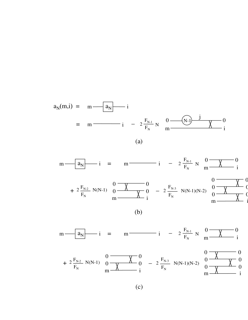
Figure 3: (a): Diagrammatic representation of eq. (34), which gives the quantity $a_{N}(m,i)$ defined in eq. (32). (b): Pauli diagrams for this $a_{N}(m,i)$. They are obtained by inserting diagrams of fig. 2c for $\zeta^{\ast}$ into fig. 3a. They contain 0,1,2,3,…Pauli scatterings represented by crosses, put in zigzag, alternatively right, left, right,…. $m$ and $i$ stay on the bottom line. Fig. 3b is just a visualization of eq. (35). Here again, as in all the Pauli diagrams, sums are taken over the intermediate (unlabelled) exciton lines. (c): Same $a_{N}(m,i)$ obtained by using $[B_{0}^{N},D_{mi}]$, instead of $[D_{mi},B_{0}^{{\dagger}N}]$, in eq. (32). This other diagrammatic representation of $a_{N}(m,i)$, in which the relative position of the crosses is just changed compared to fig. 3b, is the one useful to get $A_{N}(m,i)$ in terms of $A_{N-2}(m,j)$, as done in the last part of this work.

Fig. 3a shows the diagrammatic representation of eq. (34), while fig. 3b shows the corresponding expansion of $a_{N}(m,i)$ deduced from the diagrammatic expansion of $\zeta_{N}^{\ast}(i)$ given in fig. 2c. By injecting eq. (28) giving $\zeta_{N}(m)$ into eq. (34), we find

$$a_{N}(m,i)=\delta_{mi}+2\sum_{p=1}^{N}(-1)^{p}\,\frac{F_{N-p}}{F_{N}}\,\frac{N!}{(N-p)!}\,z^{(p)}(m,i)\ ,$$ (35)

where $z^{(p)}(m,i)$ is such that

$$z^{(p)}(m,i)=\sum_{j}\lambda_{mj0i}\,z^{(p-1)\ast}(j,0)\ .$$ (36)

As shown in fig. 3b, $z^{(p)}(m,i)$ is a zigzag diagram like $z^{(p)}(m,0)$, with the lowest line $(m,0)$ replaced by $(m,i)$.

If we now turn to $\hat{A}_{N}(i,m)$, there are a priori two ways to calculate it: Either we use $[B_{m},B_{0}^{{\dagger}N}]$, or we use $[B_{0}^{N},B_{i}^{\dagger}]$. However, if we want to write $\hat{A}_{N}(i,m)$ in terms of $A_{N-2}(n,i)$, we must keep $B_{i}^{\dagger}$ so that $[B_{0}^{N},B_{i}^{\dagger}]$ is not appropriate. Equation (23) then leads to

$$\hat{A}_{N}(i,m)=\frac{F_{N-1}}{F_{N}}\,N\,\delta_{m0}\,\zeta_{N-1}^{\ast}(i)-\frac{N(N-1)}{N!F_{N}}\sum_{j}\lambda_{mj00}\,\langle v|B_{0}^{N}B_{i}^{\dagger}B_{j}^{\dagger}B_{0}^{{\dagger}N-2}|v\rangle\ .$$ (37)

The above matrix element can be calculated either with $[B_{0}^{N},B_{j}^{\dagger}]$ or with $[B_{0}^{N},B_{i}^{\dagger}]$. From the first commutator — which is the one which allows to keep $B_{i}^{\dagger}$ — we get

$$\hat{A}_{N}(i,m)=N\,b_{N}(m,i)+\frac{F_{N-2}}{F_{N}}\,N(N-1)\sum_{nj}\lambda_{mj00}\lambda_{00nj}\,A_{N-2}(n,i)\ ,$$ (38)

in which we have set

$$b_{N}(m,i)=\frac{F_{N-1}}{F_{N}}\,\delta_{m0}\,\zeta_{N-1}^{\ast}(i)-\frac{F_{N-2}}{F_{N}}\,(N-1)\,\lambda_{m000}\,\zeta_{N-2}^{\ast}(i)\ .$$ (39)

By using the expansion of $\zeta_{N}(m)$ given in eq. (28), this equation leads to write $b_{N}(m,i)$ as

$$b_{N}(m,i)=\frac{F_{N-1}}{F_{N}}\,\delta_{m0}\,\delta_{0i}+\sum_{p=1}^{N-1}(-1)^{p}\,\frac{(N-1)!}{(N-1-p)!}\,\frac{F_{N-1-p}}{F_{N}}\hskip 85.35826pt$$

$$\times\left[z^{(0)}(m,0)\,z^{(p)\ast}(i,0)+z^{(1)}(m,0)\,z^{(p-1)\ast}(i,0)\right]\ .$$ (40)

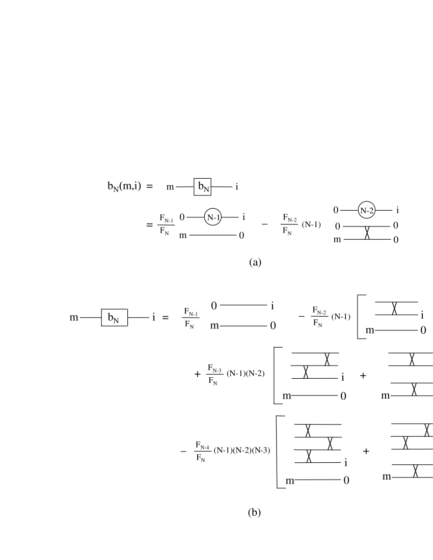
Figure 4: (a): Diagrammatic representation of eq. (39) which defines the quantity $b_{N}(m,i)$. (b): Pauli diagrams for this $b_{N}(m,i)$ obtained by inserting the diagrams of fig. 2c for $\zeta^{\ast}$ into fig. 4a. $b_{N}(m,i)$ is made of a set of disconnected diagrams, with 0,1,2,3,…Pauli scatterings represented by crosses. At each order, it contains two terms, one with a $\delta_{m0}$ factor, the other with a $\lambda_{m000}$ factor. As in the following Pauli diagrams, we have omitted the final exciton indices $0$ to simplify the figures. Fig. 4b is a simple visualization of eq. (40).

The diagrammatic representation of eq. (39) is shown in fig. 4a. From it and the diagrams of fig. 2c for $\zeta_{N}^{\ast}(i)$, we obtain the Pauli expansion of $b_{N}(m,i)$ shown in fig. 4b. It is just the diagrammatic representation of eq. (40). We see that $b_{N}(m,i)$ is made of diagrams which can be cut into two pieces. We also see that, while $a_{N}(m,i)$ differs from 0 for $\mathbf{Q}_{m}=\mathbf{Q}_{i}$ only, due to momentum conservation included in the Pauli scatterings, we must have $\mathbf{Q}_{m}=\mathbf{Q}_{i}=\mathbf{Q}_{0}$ to have $b_{N}(m,i)\neq 0$, since $\zeta_{N}(m)$ is 0 for $\mathbf{Q}_{m}\neq\mathbf{Q}_{0}$, as previously shown.

From eqs. (31) and (38), we thus find that $A_{N}(m,i)$ obeys the recursion relation

$$A_{N}(m,i)=a_{N}(m,i)+N\,b_{N}(m,i)+\frac{F_{N-2}}{F_{N}}\,N(N-1)\sum_{nj}\lambda_{mj00}\lambda_{00nj}\,A_{N-2}(n,i)\ ,$$ (41)

with $b_{N}(m,i)=0$ if $\mathbf{Q}_{m}=\mathbf{Q}_{i}\neq\mathbf{Q}_{0}$.

3.2.2 Determination of $A_{N}(m,i)$ using $A_{N-2}(n,i)$

From the fact that we just need to have $\mathbf{Q}_{m}=\mathbf{Q}_{i}$ for $a_{N}(m,i)\neq 0$, while $b_{N}(m,i)\neq 0$ imposes $\mathbf{Q}_{m}=\mathbf{Q}_{i}=\mathbf{Q}_{0}$, we are led to divide $A_{N}(m,i)$ into a contribution which exists whatever the $i$ exciton momentum is and a contribution which only exists when $\mathbf{Q}_{i}$ is equal to the sea exciton momentum $\mathbf{Q}_{0}$. This gives

$$A_{N}(m,i)=\alpha_{N}(m,i)+N\,\beta_{N}(m,i)\ ,$$ (42)

where $\alpha_{N}(m,i)$ and $\beta_{N}(m,i)$ obey the two recursion relations

$$\alpha_{N}(m,i)=a_{N}(m,i)+\frac{F_{N-2}}{F_{N}}\,N(N-1)\sum_{nj}\lambda_{mj00}\lambda_{00nj}\,\alpha_{N-2}(n,i)\ ,$$ (43)

$$\beta_{N}(m,i)=b_{N}(m,i)+\frac{F_{N-2}}{F_{N}}\,(N-1)(N-2)\sum_{nj}\lambda_{mj00}\lambda_{00nj}\,\beta_{N-2}(n,i)\ .$$ (44)

a) Part of $A_{N}(m,i)$ which exists whatever $\mathbf{Q}_{i}(=\mathbf{Q}_{m})$ is

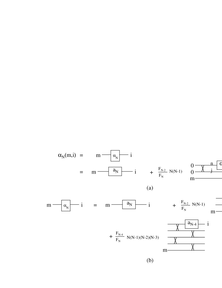
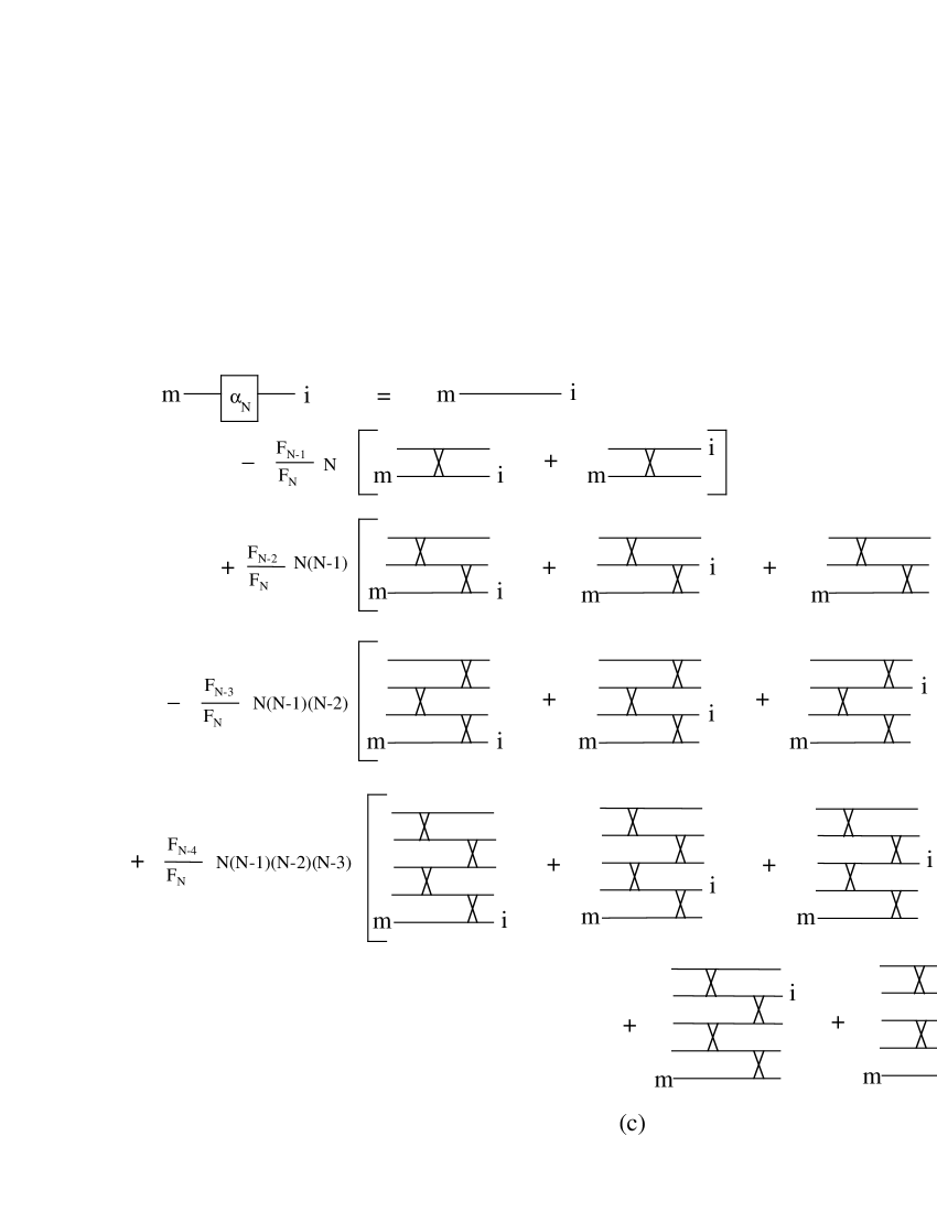
Figure 5: (a): Recursion relation (43) for the part $\alpha_{N}(m,i)$ of the scalar product $A_{N}(m,i)$ which exists even if $\mathbf{Q}_{m}=\mathbf{Q}_{i}\neq\mathbf{Q}_{0}$. (b): Iterative expansion of $\alpha_{N}(m,i)$ in terms of $a_{N}(m,i)$. (c):The Pauli diagrams for $\alpha_{N}(m,i)$, obtained by inserting the diagrammatic representation of $a_{N}(m,i)$ shown in fig. 3b, into fig. 5b, are made of zigzag diagrams with Pauli scatterings put alternatively right, left, right,…The index $m$ stays at the left bottom, while $i$ moves at all possible positions on the right. Fig. 5c is just a visualization of eq. (45).

The part of $A_{N}(m,i)$ which exists for any exciton $i$ is $\alpha_{N}(m,i)$. The diagrammatic representation of its recursion relation (43) is shown in fig. 5a, as well as its iteration (fig. 5b). If, in it, we insert the diagrammatic representation of $a_{N}(m,i)$ given in fig. 3b, we end with the diagrammatic representation of $\alpha_{N}(m,i)$ shown in fig. 5c. Note that we have used $\lambda_{mn0i}=\lambda_{mni0}$ in order to get rid of the factor 2 appearing in $a_{N}(m,i)$. Using eq. (35) for $a_{N}(m,i)$, it is easy to check that the solution of eq. (43) reads

$$\alpha_{N}(m,i)=\sum_{p=0}^{N}(-1)^{p}\,\frac{F_{N-p}}{F_{N}}\,\frac{N!}{(N-p)!}\,Z^{(p)}(m,i)\ ,$$ (45)

where $Z^{(p)}(m,i)$ obeys the recursion relation

$$Z^{(p)}(m,i)=\hat{z}^{(p)}(m,i)+\sum_{nj}\lambda_{mj00}\,\lambda_{00nj}\,Z^{(p-2)}(n,i)\ ,$$ (46)

with $\hat{z}^{(0)}=\delta_{mi}$, while $\hat{z}^{(p\neq 0)}(m,i)=2z^{(p)}(m,i)$. In agreement with fig. 5c, this leads to represent $Z^{(p)}(m,i)$ as a sum of zigzag diagrams with $p$ Pauli scatterings, located alternatively right, left, right,…, the index $m$ being always at the left bottom, while $i$ can be at all possible places on the right. $Z^{(p)}(m,i)$ thus contains $(p+1)$ diagrams which reduce to one, namely $Z^{(0)}(m,i)=\delta_{mi}$, when $p=0$.

From fig. 5c, we also see that $\alpha_{N}(m,i)$ contains as many $N$’s as $\lambda$’s so that it ultimately depends on $(N,\lambda)$’s through $\eta$.

b) Part of $A_{N}(m,i)$ which exists for $\mathbf{Q}_{i}(=\mathbf{Q}_{m})=\mathbf{Q}_{0}$ only

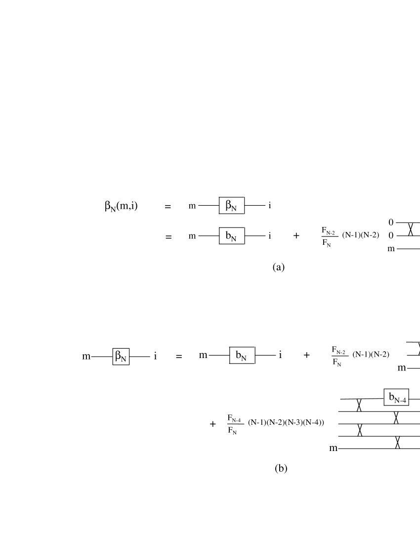
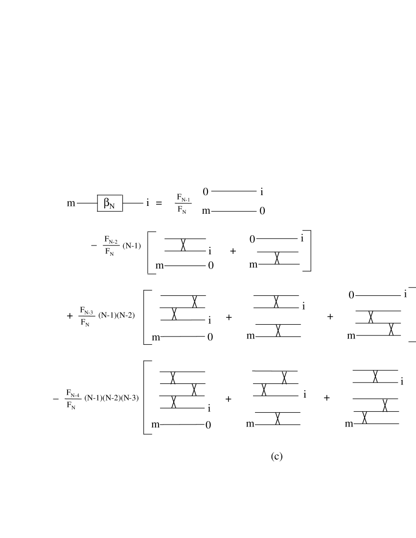
Figure 6: (a): Recursion relation (44) for the part $\beta_{N}(m,i)$ of the scalar product $A_{N}(m,i)$ which exists for $\mathbf{Q}_{m}=\mathbf{Q}_{i}=\mathbf{Q}_{0}$ only. (b): Iterative expansion of $\beta_{N}(m,i)$ in terms of $b_{N}(m,i)$. (c): Pauli diagrams for $\beta_{N}(m,i)$ obtained by inserting the diagrammatic representation of $b_{N}(m,i)$ shown in fig. 4b, into fig. 6b. $\beta_{N}(m,i)$ is made of disconnected diagrams, the two pieces being zigzag diagrams right, left, right,…for the part with $m$ at the left bottom, and left, right, left,…for the part with $i$ at the right bottom. Fig. 6c is just a visualization of eq. (47).

The part of $A_{N}(m,i)$ which only exists when the $i$ and $m$ excitons have the same momentum as the sea exciton one, is $N\,\beta_{N}(m,i)$. The diagrammatic representation of the recursion relation (44) for $\beta_{N}$ is shown in fig. 6a, as well as its iteration (fig. 6b). Using eq. (40) for $b_{N}(m,i)$ and eq. (29), it is easy to check that the solution of the recursion relation (44) reads

$$\beta_{N}(m,i)=\sum_{p=0}^{N-1}(-1)^{p}\,\frac{F_{N-1-p}}{F_{N}}\,\frac{(N-1)!}{(N-1-p)!}\,\sum_{q=0}^{p}z^{(q)}(m,0)\,z^{(p-q)\ast}(i,0)\ .$$ (47)

This is exactly what we get if, in the expansion of $\beta_{N}(m,i)$ in terms of $b_{N}(n,i)$ shown in fig. 6b, we insert the expansion of $b_{N}(n,i)$ in terms of Pauli scatterings shown in fig. 4b, (see fig. 6c): The diagrams making $\beta_{N}(m,i)$ are thus made of two pieces, in agreement with eq. (47). We also see that $\beta_{N}(m,i)$ contains as many $N$’s as $\lambda$’s so that $\beta_{N}(m,i)$, like $\alpha_{N}(m,i)$, is an $\eta$ function.

c) $N$ dependence of $A_{N}(m,i)$

If we now come back to the expression (41) for $A_{N}(m,i)$, we see that when $\beta_{N}(m,i)=0$, i. e., when $\mathbf{Q}_{m}=\mathbf{Q}_{i}\neq\mathbf{Q}_{0}$, the $N$’s in $A_{N}(m,i)$ simply appear through products $N\lambda$. On the opposite, $A_{N}(m,i)$ contains an extra prefactor $N$ when $\beta_{N}(m,i)\neq 0$, i. e., when $\mathbf{Q}_{m}=\mathbf{Q}_{i}=\mathbf{Q}_{0}$: This extra $N$ is the memory of the bosonic enhancement found for the dressed exciton $i=0$. As already explained above, this bosonic enhancement exists not only for the exciton $i=0$, but also for any exciton which can be transformed into a $0$ exciton by Pauli scatterings with the sea excitons.

From a mathematical point of view, this extra $N$ is linked to the topology of the diagrams representing $A_{N}(m,i)$. As in the case of the well known Feynman diagrams for which superextensive terms are linked to disconnected diagrams, we here see that an extra factor $N$ appears in the part of $A_{N}(m,i)$ corresponding to diagrams which are made of two pieces.

To conclude, we can say that the procedure we have used to calculate $A_{N}(m,i)$ led us to represent this scalar product by Pauli diagrams which are actually quite simple: The part of $A_{N}(m,i)$ which exists for any $\mathbf{Q}_{m}=\mathbf{Q}_{i}$ is made of all connected diagrams with $m$ at the left bottom and $i$ at all possible places on the right, the exciton lines being connected by Pauli scatterings put in zigzag right, left, right…(see fig. 5c). $A_{N}(m,i)$ has an additional part when the $m$ and $i$ excitons have a momentum equal to the sea exciton momentum $\mathbf{Q}_{0}$. This additional part is made of all possible Pauli diagrams which can be cut into two pieces, $m$ staying at the left bottom of one piece, while $i$ stays at the right bottom of the other piece, the exciton lines being connected by Pauli scatterings in zigzag right, left, right…for the $m$ piece, and left, right, left…for the $i$ piece (see fig. 6c). As a direct consequence of the topology of these diconnected diagrams, an extra factor $N$ appears in this part of $A_{N}(m,i)$. This factor $N$ is physically linked to the well known bosonic enhancement which, for composite excitons, exists not only for an exciton identical to a sea exciton, but also for any exciton which can be transformed into a sea exciton by Pauli scatterings with the sea.

Although this result for the scalar product of $(N+1)$-exciton states, with $N$ of them in the same state $0$, is nicely simple at any order in Pauli interaction, it does not leave us completely happy. Indeed, while in the diagrams which exist for $\mathbf{Q}_{i}=\mathbf{Q}_{m}=\mathbf{Q}_{0}$, the $m$ and $i$ indices play similar roles, their roles in the diagrams which exist even if $\mathbf{Q}_{i}\neq\mathbf{Q}_{0}$ are dissymmetric, which is not at all satisfactory. This dissymmetry can be traced back to the way we calculated $A_{N}(m,i)$. It is clear that equivalences between Pauli diagrams have to exist in order to restore the intrinsic $(m,i)$ symmetry of $A_{N}(m,i)$. In the last part of this work, we are going to discuss some of these equivalences between Pauli diagrams.

However, the reader, not as picky as us, may just drop this last part since, after all, the quite simple, although dissymmetric, Pauli diagrams obtained above are enough to get the correct answer for $A_{N}(m,i)$ at any order in the Pauli interactions.

4 Equivalence between Pauli diagrams

In order to have some ideas about which kinds of Pauli diagrams can be equivalent, let us first derive the other possible diagrammatic representations of $A_{N}(m,i)$. They use the recursion relations between $A_{N}(m,i)$ and $A_{N-2}(m,j)$ or $A_{N-2}(n,j)$, instead of $A_{N-2}(n,i)$.

4.1 Pauli diagrams for $A_{N}(m,i)$ using $A_{N-2}(m,j)$

To get this recursion relation, we must keep $B_{m}$ in the calculation of $\hat{A}_{N}(m,i)$ defined in eq. (33). This leads us to use $[B_{0}^{N},B_{i}^{\dagger}]$ instead of $[B_{m},B_{0}^{{\dagger}N}]$; equation (38) is then replaced by

$$\hat{A}_{N}(m,i)=N\,c_{N}(m,i)+\frac{F_{N-2}}{F_{N}}\,N(N-1)\,\sum_{nj}\lambda_{nj00}\,\lambda_{00in}\,A_{N-2}(m,j)\ ,$$ (48)

in which we have set

$$c_{N}(m,i)=\frac{F_{N-1}}{F_{N}}\,\delta_{0i}\,\zeta_{N-1}(m)-\frac{F_{N-2}}{F_{N}}\,(N-1)\lambda_{000i}\,\zeta_{N-2}(m)\ .$$ (49)

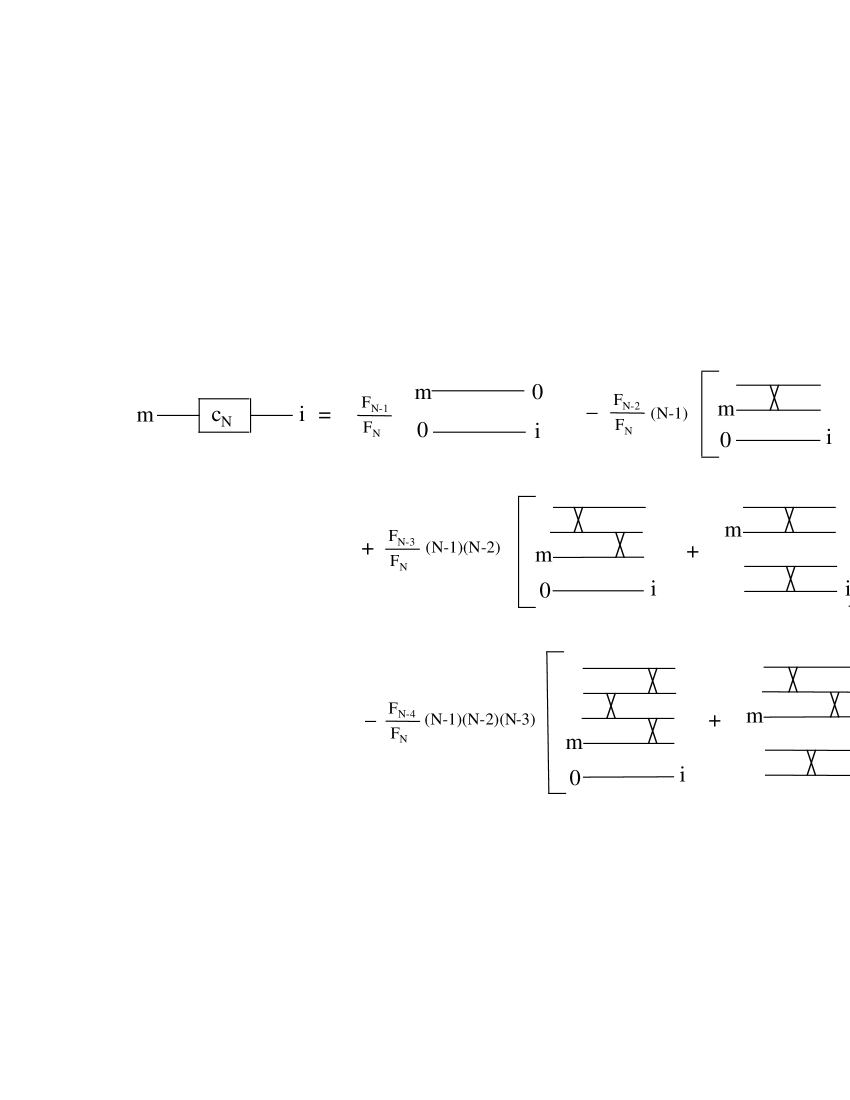
Figure 7: Pauli diagrams for $c_{N}(m,i)$ defined in eq. (49). This $c_{N}(m,i)$ appears instead of $b_{N}(m,i)$ when we want to write $A_{N}(m,i)$ in terms of $A_{N-2}(m,j)$ and not in terms of $A_{N-2}(n,i)$. As $b_{N}(m,i)$, $c_{N}(m,i)$ is made of disconnected diagrams. At each order, it contains two terms, one with a $\delta_{i0}$ factor, the other with a $\lambda_{000i}$ factor.

Using fig. 2b for $\zeta_{N}(m)$, we easily obtain the diagrams for $c_{N}(m,i)$ shown in fig. 7. When compared to $b_{N}(m,i)$, we see that the roles played by $m$ and $i$ are exchanged as well as the relative position of the crosses.

Equation (48) leads to write $A_{N}(m,i)$ as

$$A_{N}(m,i)=\overline{\alpha}_{N}(m,i)+N\,\overline{\beta}_{N}(m,i)\ ,$$ (50)

where $\overline{\alpha}_{N}(m,i)$ and $\overline{\beta}_{N}(m,i)$ obey the recursion relations

$$\overline{\alpha}_{N}(m,i)=a_{N}(m,i)+\frac{F_{N-2}}{F_{N}}\,N(N-1)\,\sum_{nj}\lambda_{nj00}\,\lambda_{00in}\,\overline{\alpha}_{N-2}(m,j)\ ,$$ (51)

$$\overline{\beta}_{N}(m,i)=c_{N}(m,i)+\frac{F_{N-2}}{F_{N}}\,(N-1)(N-2)\,\sum_{nj}\lambda_{nj00}\,\lambda_{00in}\,\overline{\beta}_{N-2}(m,j)\ .$$ (52)

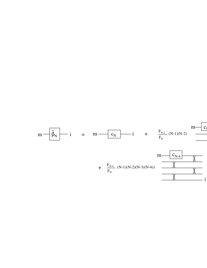
Figure 8: Diagrammatic representation of the $\overline{\beta}_{N}(m,i)$ part of $A_{N}(m,i)$ which exists for $\mathbf{Q}_{m}=\mathbf{Q}_{i}=\mathbf{Q}_{0}$ only, as it appears when we use the recursion relation between $A_{N}(m,i)$ and $A_{N-2}(m,j)$, instead of $A_{N-2}(n,i)$. This diagrammatic representation corresponds to the iteration of eq. (52). By inserting the diagrams for $c_{N}(m,i)$, shown in fig. 7, in this fig. 8, it is straightforward to see that the Pauli diagrams for $\overline{\beta}_{N}(m,i)$ are identical to the ones for $\beta_{N}(m,i)$ at any order in Pauli scatterings, so that $\overline{\beta}_{N}(m,i)=\beta_{N}(m,i)$.

Let us first consider $\overline{\beta}_{N}(m,i)$. As $\beta_{N}(m,i)$, it differs from zero for $\mathbf{Q}_{m}=\mathbf{Q}_{i}=\mathbf{Q}_{0}$ only. Its recursion relation leads to expand it in terms of $c$’s as shown in fig. 8. If we now replace the $c$’s by their expansion shown in fig. 7, we immediately find that $\overline{\beta}_{N}(m,i)$ is represented by the same Pauli diagrams as the ones for $\beta_{N}(m,i)$, so that $\overline{\beta}_{N}(m,i)=\beta_{N}(m,i)$. This is after all not surprising because, in them, the roles played by $m$ and $i$ are symmetrical.

From this result, we immediately conclude that the parts of $A_{N}(m,i)$ which exist even if $\mathbf{Q}_{i}=\mathbf{Q}_{m}\neq\mathbf{Q}_{0}$ have also to be equal, i. e., we must have $\overline{\alpha}_{N}(m,i)=\alpha_{N}(m,i)$. Let us now see how this $\overline{\alpha}_{N}(m,i)$ appears, using eq. (51).

If we calculate $a_{N}(m,i)$ not with $[D_{mi},B_{0}^{{\dagger}N}]$ but with $[B_{0}^{N},D_{mi}]$, we find that $a_{N}(m,i)$ can be represented, not only by the diagrams of fig. 3b, but also by those of fig. 3c. These diagrams look very similar, except that the crosses are now in zigzag left, right, left…Since these two sets of diagrams (3b) and (3c) represent the same $a_{N}(m,i)$, while they have to be valid for $N=2,3,\cdots$, the relative positions of the crosses have to be unimportant in these Pauli diagrams. We will come back to this equivalence at the end of this part.

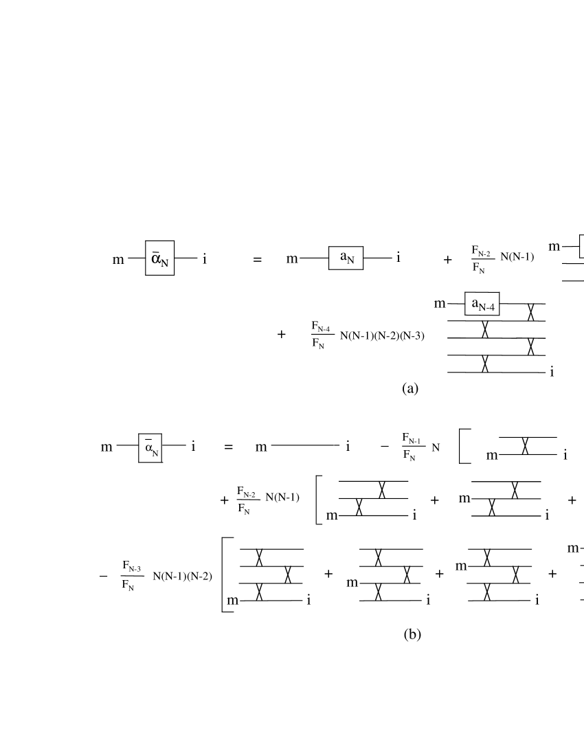
Figure 9: (a): Diagrammatic representation of the $\overline{\alpha}_{N}(m,i)$ part of $A_{N}(m,i)$ which exists even if $\mathbf{Q}_{m}=\mathbf{Q}_{i}\neq\mathbf{Q}_{0}$, as it appears when we use the recursion relation between $A_{N}(m,i)$ and $A_{N-2}(m,j)$. This diagrammatic representation corresponds to the iteration of eq. (51). (b): Pauli diagrams for this $\overline{\alpha}_{N}(m,i)$ as obtained by inserting the diagrams of fig. 3c for $a_{N}(m,i)$ into fig. 9a. These diagrams look like the ones for $\alpha_{N}(m,i)$, shown in fig. 5c, except that the zigzags are now left, right, left, …, with $i$ staying at the right bottom and $m$ moving at all possible positions on the left. Since $\overline{\beta}_{N}(m,i)=\beta_{N}(m,i)$, we do have $\overline{\alpha}_{N}(m,i)=\alpha_{N}(m,i)$ for any $N$; so that the two sets of Pauli diagrams for $\overline{\alpha}_{N}(m,i)$ and $\alpha_{N}(m,i)$ must actually correspond to the same quantity, at any order in Pauli scatterings. This will be proved later on.

The iteration of the recursion relation for $\overline{\alpha}_{N}(m,i)$ leads to the diagrams of fig. 9a. If in them, we insert the diagrams of fig. 3c for $a_{N}(m,i)$, we get the diagrams of fig. 9b. They look like the ones for $\alpha_{N}(m,i)$, except that $i$ now stays at the right bottom while $m$ moves to all possible positions on the left, the zigzag for the Pauli scatterings being now left, right, left…This leads to write $\overline{\alpha}_{N}(m,i)$ as

$$\overline{\alpha}_{N}(m,i)=\sum_{p=0}^{N}(-1)^{p}\,\frac{F_{N-p}}{F_{N}}\,\frac{N!}{(N-p)!}\,\overline{Z}^{(p)}(m,i)\ ,$$ (53)

where $\overline{Z}^{(p)}(m,i)$ represents the set of zigzag diagrams of fig. 9b, with $p$ crosses.

Since $\overline{\alpha}_{N}(m,i)=\alpha_{N}(m,i)$, we conclude from the validity of their expansions for $N=2,3,\cdots$, that the zigzag diagrams $Z^{(p)}(m,i)$ and $\overline{Z}^{(p)}(m,i)$ must correspond to identical quantities, which is not obvious at first.

4.2 Pauli diagrams for $A_{N}(m,i)$ using $A_{N-2}(n,j)$

To get this recursion relation, we start as for the one between $A_{N}(m,i)$ and $A_{N-2}(n,i)$, but we use $[B_{0}^{N},B_{i}^{\dagger}]$ instead of $[B_{0}^{N},B_{j}^{\dagger}]$ to calculate the matrix element appearing in eq. (37). This leads to

$$\hat{A}_{N}(m,i)=N\,d_{N}(m,i)+\frac{F_{N-2}}{F_{N}}\,N(N-1)\,\sum_{nj}\lambda_{mj00}\,\lambda_{00ni}\,A_{N-2}(n,j)\ ,$$ (54)

in which we have set

$$d_{N}(m,i)=\frac{F_{N-1}}{F_{N}}\,\delta_{m0}\,\zeta_{N-1}^{\ast}(i)-\frac{F_{N-2}}{F_{N}}\,(N-1)\,\delta_{0i}\,\sum_{j}\lambda_{mj00}\,\zeta_{N-2}^{\ast}(j)\ .$$ (55)

Using the diagrams of fig. 2c for $\zeta_{N}^{\ast}(i)$, it is easy to show that $d_{N}(m,i)$ is represented by the diagrams of fig. 10. Note that they are different from the ones for $b_{N}(m,i)$ and $c_{N}(m,i)$ shown in fig. 4b and fig. 7. This is actually normal because, as seen from eq. (55), $d_{N}(m,i)$ is equal to zero when both $m\neq 0$ and $i\neq 0$, while $b_{N}(m,i)$ and $c_{N}(m,i)$ differ from zero provided that $\mathbf{Q}_{m}(=\mathbf{Q}_{i})$ is equal to $\mathbf{Q}_{0}$.

Equation (54) leads to write $A_{N}(m,i)$ as

$$A_{N}(m,i)=\overline{\overline{\alpha}}_{N}(m,i)+N\,\overline{\overline{\beta}}_{N}(m,i)\ ,$$ (56)

where $\overline{\overline{\alpha}}_{N}(m,i)$ and $\overline{\overline{\beta}}_{N}(m,i)$ now obey

$$\overline{\overline{\alpha}}_{N}(m,i)=a_{N}(m,i)+\frac{F_{N-2}}{F_{N}}\,N(N-1)\,\sum_{nj}\lambda_{mj00}\,\lambda_{00ni}\,\overline{\overline{\alpha}}_{N-2}(n,j)\ ,$$ (57)

$$\overline{\overline{\beta}}_{N}(m,i)=d_{N}(m,i)+\frac{F_{N-2}}{F_{N}}\,(N-1)(N-2)\,\sum_{nj}\lambda_{mj00}\,\lambda_{00ni}\,\overline{\overline{\beta}}_{N-2}(n,j)\ .$$ (58)

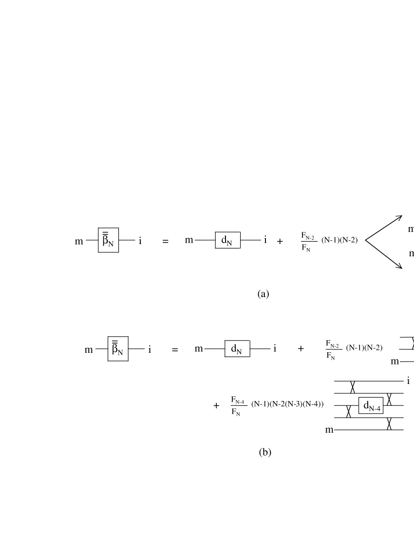
Figure 11: (a): The two possible representations of the same recursion relation (58) for the $\overline{\overline{\beta}}_{N}(m,i)$ part of $A_{N}(m,i)$ which exists for $\mathbf{Q}_{m}=\mathbf{Q}_{i}=\mathbf{Q}_{0}$ only, as it appears when we use the recursion relation between $A_{N}(m,i)$ and $A_{N-2}(n,j)$ instead of $A_{N-2}(n,i)$. These two representations just result from a symmetry up-down which follows from fig. 1c, since $\lambda_{mnij}=\lambda_{nmji}$. (b): Iteration of this recursion relation. The two representations of $\overline{\overline{\beta}}_{N}(m,i)$ shown in fig. 11a have been alternatively used in order to avoid the crossings of the exciton lines. If, in this fig. 11b, we insert the diagrams of fig. 10 for $d_{N}(m,i)$, we immediately find that the Pauli diagrams for $\overline{\overline{\beta}}_{N}(m,i)$ are exactly those of $\beta_{N}(m,i)$, so that $\overline{\overline{\beta}}_{N}(m,i)=\beta_{N}(m,i)$.

Let us start with $\overline{\overline{\beta}}_{N}(m,i)$. Its recursion relation is shown in fig. 11a, as well as its iteration (fig. 11b). (In it, we have used the two equivalent forms of this recursion relation given in fig. 11a). If, in these diagrams, we now insert the diagrammatic representation of $d_{N}(m,i)$ shown in fig. 10, with the $m$ part alternatively below and above the $i$ part, we find that $\overline{\overline{\beta}}_{N}(m,i)$ is represented by exactly the same diagrams as the ones for $\beta_{N}(m,i)$, so that $\overline{\overline{\beta}}_{N}(m,i)=\beta_{N}(m,i)$. As a consequence, we must have $\overline{\overline{\alpha}}_{N}(m,i)=\alpha_{N}(m,i)$.

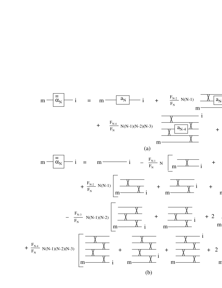
Figure 12: (a): Diagrammatic representation of the $\overline{\overline{\alpha}}_{N}(m,i)$ part of $A_{N}(m,i)$ which exists even if $\mathbf{Q}_{m}=\mathbf{Q}_{i}\neq\mathbf{Q}_{0}$, as it appears when we use the recursion relation between $A_{N}(m,i)$ and $A_{N-2}(n,j)$. This diagrammatic representation corresponds to the iteration of eq. (57). (b): Pauli diagrams for this $\overline{\overline{\alpha}}_{N}(m,i)$ as obtained by inserting the diagrams of fig. 3b for $a_{N}(m,i)$ into fig. 12a. The zeroth, first and second order Pauli diagrams of $\overline{\overline{\alpha}}_{N}(m,i)$ are identical to the ones of $\alpha_{N}(m,i)$ shown in fig. 5c. On the opposite, at higher orders, these Pauli diagrams become more and more different. They however have to represent exactly the same quantity, since $\overline{\overline{\beta}}_{N}(m,i)=\beta_{N}(m,i)$, so that we do have $\overline{\overline{\alpha}}_{N}(m,i)=\alpha_{N}(m,i)$ for any $N$.

Let us now consider the recursion relation between $\overline{\overline{\alpha}}_{N}(m,i)$ and $\overline{\overline{\alpha}}_{N-2}(n,j)$. The iteration of this recursion relation leads to the diagrams of fig. 12a. If in it, we insert the diagrammatic representation of $a_{N}(m,i)$ shown in fig. 3b, we get the diagrams of fig. 12b. We can note that it is not enough to use $\lambda_{0n00}=\lambda_{n000}$ to transform the last third order diagram into the two last third order zigzag diagrams left, right, left of $\alpha_{N}(m,i)$. At fourth order, the situation is even worse, the last fourth order Pauli diagram for $\overline{\overline{\alpha}}_{N}(m,i)$ being totally different from a zigzag diagram. They however have to represent the same quantity because $\overline{\overline{\alpha}}_{N}(m,i)=\alpha_{N}(m,i)$ for any $N$.

Let us now identify the underlying reason for the equivalence of Pauli diagrams like the ones of figs. 3b and 3c which represent the same $a_{N}(m,i)$, or the ones of figs. 5c, 9b and 12b which represent the part of the same $A_{N}(m,i)$ which exists even if $\mathbf{Q}_{m}(=\mathbf{Q}_{i})\neq\mathbf{Q}_{0}$. This will help us to understand how these Pauli diagrams really work.

4.3 “Exchange skeletons”

All the Pauli diagrams we found in the preceding sections, are made of a certain number of exciton lines connected by Pauli scatterings between two excitons, put in various orders. It is clear that the value of these diagrams can depend on the “in” and “out” exciton states, i. e., the indices which appear at the right and the left of these diagrams, but not on the intermediate exciton states over which sums are taken. Between these “in” and “out” excitons, a lot of carrier exchanges take place through the various Pauli scatterings represented by crosses in the Pauli diagrams. It is actually reasonable to think that these Pauli diagrams have to ultimately read in terms of “exchange skeletons” between the “in” and “out” excitons of these diagrams. For $N=2,3,4,$…excitons, these “exchange skeletons” should appear as

$$L^{(2)}(m_{1},m_{2};i_{1},i_{2})=\int d\mathbf{r}_{e_{1}}\cdots d\mathbf{r}_{h_{2}}\phi_{m_{1}}^{\ast}(\mathbf{r}_{e_{1}},\mathbf{r}_{h_{1}})\phi_{m_{2}}^{\ast}(\mathbf{r}_{e_{2}},\mathbf{r}_{h_{2}})\phi_{i_{1}}(\mathbf{r}_{e_{1}},\mathbf{r}_{h_{2}})\phi_{i_{2}}(\mathbf{r}_{e_{2}},\mathbf{r}_{h_{1}}),$$ (59)

$$L^{(3)}(m_{1},m_{2},m_{3};i_{1},i_{2},i_{3})=\int d\mathbf{r}_{e_{1}}\cdots d\mathbf{r}_{h_{3}}\phi_{m_{1}}^{\ast}(\mathbf{r}_{e_{1}},\mathbf{r}_{h_{1}})\phi_{m_{2}}^{\ast}(\mathbf{r}_{e_{2}},\mathbf{r}_{h_{2}})\phi_{m_{3}}^{\ast}(\mathbf{r}_{e_{3}},\mathbf{r}_{h_{3}})$$

$$\times\phi_{i_{1}}(\mathbf{r}_{e_{1}},\mathbf{r}_{h_{2}})\phi_{i_{2}}(\mathbf{r}_{e_{3}},\mathbf{r}_{h_{1}})\phi_{i_{3}}(\mathbf{r}_{e_{2}},\mathbf{r}_{h_{3}}),$$ (60)

$$L^{(4)}(m_{1},m_{2},m_{3},m_{4};i_{1},i_{2},i_{3},i_{4})=\int d\mathbf{r}_{e_{1}}\cdots d\mathbf{r}_{h_{4}}\phi_{m_{1}}^{\ast}(\mathbf{r}_{e_{1}},\mathbf{r}_{h_{1}})\phi_{m_{2}}^{\ast}(\mathbf{r}_{e_{2}},\mathbf{r}_{h_{2}})\hskip 56.9055pt$$

$$\times\phi_{m_{3}}^{\ast}(\mathbf{r}_{e_{3}},\mathbf{r}_{h_{3}})\phi_{m_{4}}^{\ast}(\mathbf{r}_{e_{4}},\mathbf{r}_{h_{4}})\phi_{i_{1}}(\mathbf{r}_{e_{1}},\mathbf{r}_{h_{2}})\phi_{i_{2}}(\mathbf{r}_{e_{3}},\mathbf{r}_{h_{1}})\phi_{i_{3}}(\mathbf{r}_{e_{2}},\mathbf{r}_{h_{4}})\phi_{i_{4}}(\mathbf{r}_{e_{4}},\mathbf{r}_{h_{3}}),$$ (61)

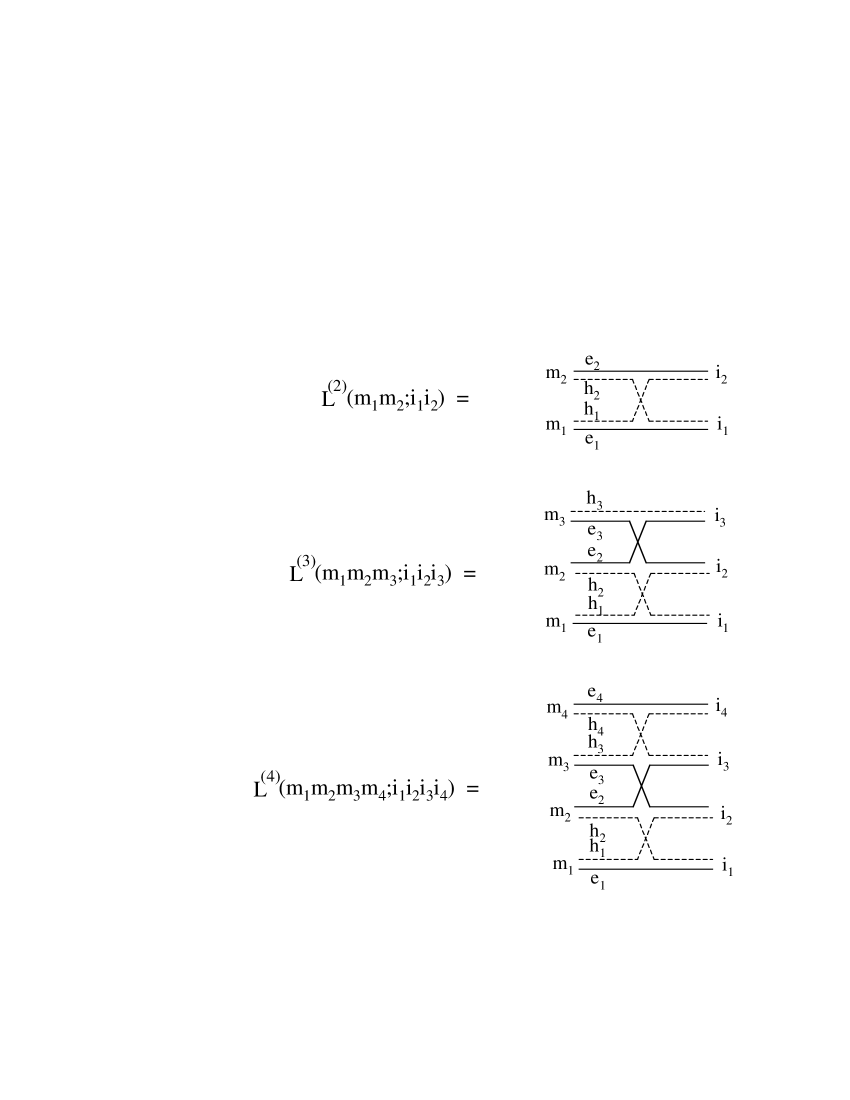
Figure 13: “Exchange skeletons” between 2,3 and 4 excitons, as defined in eqs. (59-61).

and so on…These definitions are actually transparent once we look at the diagrammatic representations of these exchange skeletons shown in fig. 13.

There are in fact various equivalent ways to represent these exchange skeletons, as can be seen from fig. 14 in the case of three excitons. These equivalent representations simply say that the $i_{1}$ exciton has the same electron as the $m_{1}$ exciton and the same hole as the $m_{2}$ exciton, so that $i_{1}$ and $m_{1}$ must be connected by an electron line while $i_{1}$ and $m_{2}$ must be connected by a hole line.

All possible carrier exchanges between $N$ excitons can be expressed in terms of these exchange skeletons.

• In the case of two excitons, the Pauli scattering which appears in the Pauli diagrams, is just $\lambda_{mnij}=\left(L^{(2)}(m,n;i,j)+L^{(2)}(n,m;i,j)\right)/2$ (see fig. 1a). In our many-body theory for interacting composite bosons, this $\lambda_{mnij}$ appears as composed of processes in which the indices $m$ and $n$ are exchanged. This is actually equivalent to say that the excitons exchange their electrons instead of their holes (see fig. 1b). We can also note that, when the two indices on one side are equal, like in $\lambda_{mn00}$, to exchange an electron or to exchange a hole is just the same (see figs. 1d and 1e).

• For three excitons, we could think of a carrier exchange between the $(i,j,k)$ and $(m,n,p)$ excitons, different from the one corresponding to $L^{(3)}(m,n,p;i,j,k)$. Let us, for example, consider the one which would read like eq. (60), with $(m_{1},m_{2},m_{3},i_{1})$ respectively replaced by $(m,n,p,i)$, while $\phi_{i_{2}}(\mathbf{r}_{e_{3}},\mathbf{r}_{h_{1}})\phi_{i_{3}}(\mathbf{r}_{e_{2}},\mathbf{r}_{h_{3}})$ is replaced by $\phi_{j}(\mathbf{r}_{e_{2}},\mathbf{r}_{h_{3}})\phi_{k}(\mathbf{r}_{e_{3}},\mathbf{r}_{h_{1}})$. This carrier exchange, shown in fig. 15, indeed reads as an exchange skeleton, being simply $L^{(3)}(m,n,p;i,k,j)$.

  And so on, for any other carrier exchange we could think of.

Let us now consider the various diagrams we have found in calculating $A_{N}(m,i)$ and understand why they are indeed equivalent, in the light of these exchange skeletons.

4.4 Pauli diagrams with one exciton only different from 0

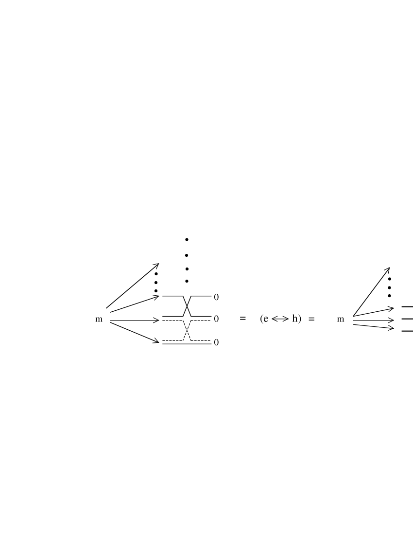
Figure 16: When all the indices of an exchange skeleton are equal, except one, the position of this $m$ index can be in any place. This exchange skeleton actually represents all Pauli diagrams with $m$ at any place on the left. The relative positions of the crosses are also unimportant, due to possible “slidings” of the carrier exchanges, as shown in the next fig. 17 for the particular case of three excitons.

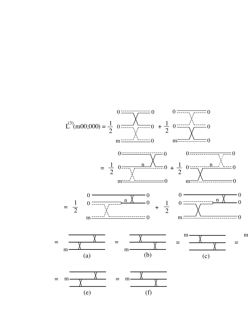
Figure 17: The exchange skeleton for three excitons $L^{(3)}(m00;000)$, with all excitons except one in the same state, corresponds to one of the two equivalent diagrams of the first line, so that it is also half their sum. In the second line, we have just “slided” the carrier exchanges. We then use the fact that, when the two indices on one side of a Pauli scattering are equal, this Pauli scattering, here $\lambda_{n000}$, corresponds either to an electron exchange or to a hole exchange. Finally, we use the representation of fig. 1a for $\lambda_{m00n}$ to get the Pauli diagram shown in (a). If we slide the carrier exchanges the other way, we get the Pauli diagram (b). The diagram (c) is obtained from (a) by a symmetry up-down which follows from $\lambda_{mnij}=\lambda_{nmji}$; and similarly for diagram (d) starting from (b). In the same way, the diagram (e) follows from (a) due to $\lambda_{m00n}=\lambda_{0m0n}$, while the diagram (f) follows from (c) for the same reason. All this shows that the Pauli diagrams with only one index different from $0$, correspond to the same exchange skeleton, whatever the positions of $m$ and the Pauli scatterings are.

We first take the simplest of these Pauli diagrams, namely the zigzag diagram $z^{(p)}(m,0)$ entering $\zeta_{N}(m)$, shown in fig. 2. On its left, this zigzag diagram has $p$ excitons $0$ and one exciton $m$, while on its right, the $(p+1)$ excitons are all $0$ excitons. After summation over the intermediate exciton indices, the final expression of this Pauli diagram must read as an integral of $\phi_{m}^{\ast}(\mathbf{r}_{e_{1}},\mathbf{r}_{h_{1}})\phi_{0}^{\ast}(\mathbf{r}_{e_{2}},\mathbf{r}_{h_{2}})$ …$\phi_{0}^{\ast}(\mathbf{r}_{e_{p+1}},\mathbf{r}_{h_{p+1}})$ multiplied by $(p+1)$ wave functions $\phi_{0}$ with the $(\mathbf{r}_{e_{i}},\mathbf{r}_{h_{i}})$’s mixed in such a way that the integral cannot be cut into two independent integrals (otherwise the Pauli diagram would be topologically disconnected). This is exactly what the exchange skeleton $L^{(p+1)}(m,0\cdots,0;0,\cdots,0)$ does.The possible permutations of the various $(\mathbf{r}_{e},\mathbf{r}_{h})$’s in the definition of this $L^{(p+1)}$, actually show that the $m$ index in the diagrammatic representation of this exchange skeleton can be in any possible place on the left. This is also true for the $m$ position in the Pauli diagrams with all the indices equal to $0$ except one. Moreover, the relative position of the crosses in these diagrams are unimportant (see fig. 16). This is easy to show, just by “sliding” the carrier exchanges, as explicitly shown in the case of three excitons (see fig. 17). In this figure, we have also used the fact that the Pauli scatterings reduce to one diagram when the two indices on one side are equal (see figs. 1d and 1e). This possibility to “slide” the carrier exchange, mathematically comes from the fact that $\sum_{q}\phi_{q}^{\ast}(\mathbf{r}_{e},\mathbf{r}_{h})\phi_{q}(\mathbf{r}_{e^{\prime}},\mathbf{r}_{h^{\prime}})$ is nothing but $\delta(\mathbf{r}_{e}-\mathbf{r}_{e^{\prime}})\delta(\mathbf{r}_{h}-\mathbf{r}_{h^{\prime}})$.

4.5 Pauli diagrams with one exciton on each side different from 0

There are essentially two kinds of such diagrams: Either the two excitons $(m,i)$ different from $0$ have no common carrier, or they have one. Let us start with this second case.

4.5.1 $m$ and $i$ have one common carrier

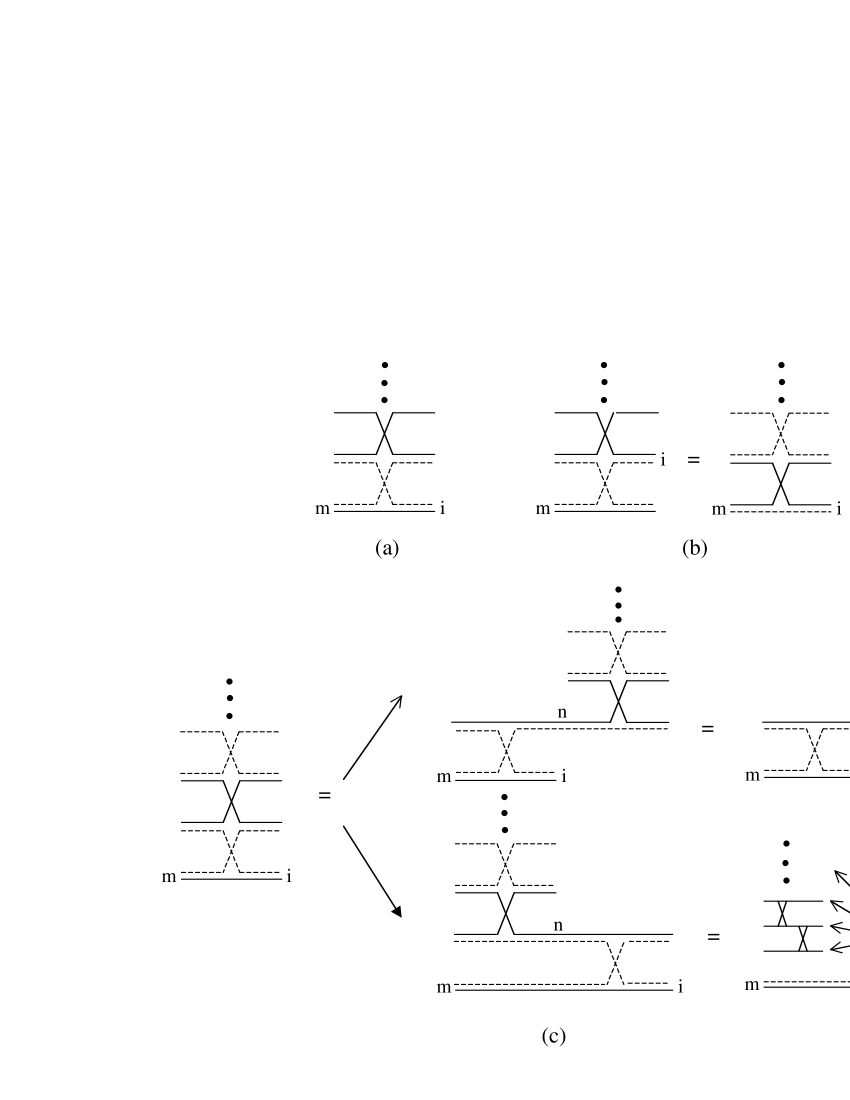
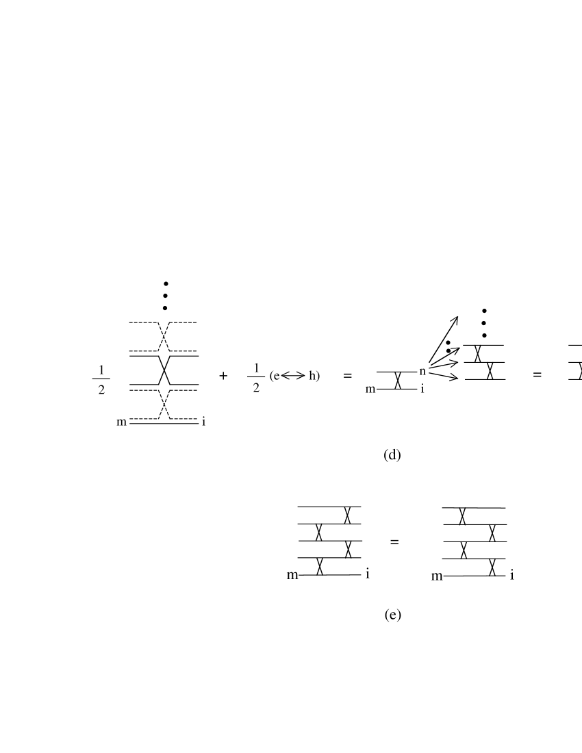
Figure 18: (a,b): Exchange skeletons for which the $m$ and $i$ excitons have the same electron (a) and the same hole (b). (c): When all the other indices are $0$, we can slide the carrier exchange one way or the other to identify an exchange skeleton for which all the indices are $0$ except one; so that it represents Pauli diagrams with the $n$ index and the crosses for Pauli scatterings at any place, as shown in fig. 16. (d,e): If we now add the electron exchange and the hole exchange to restore a full $\lambda_{m0in}$ or $\lambda_{mni0}$ Pauli scattering, we easily identify the set of Pauli diagrams which represent the same quantity. This in particular shows that the two Pauli diagrams shown in (e), which appear in the two possible ways to calculate $a_{N}(m,i)$, namely the diagrams of figs. 3b and 3c, are indeed equal.

Two different exchange skeletons exist in this case, depending if the common carrier is an electron or a hole. They are shown in figs. 18a and 18b. By “sliding” the carrier exchanges as done in fig. 18c, it is easy to identify the set of Pauli diagrams which correspond to the sum of these two exchange skeletons (see fig. 18d). This in particular shows the identity of the Pauli diagrams of fig. 18e which enter the two diagrammatic representations of $a_{N}(m,i)$ shown in figs. 3b and 3c.

4.5.2 $m$ and $i$ do not have a common carrier

In this case, the number of different exchange skeletons depends on the number of $0$ excitons involved.

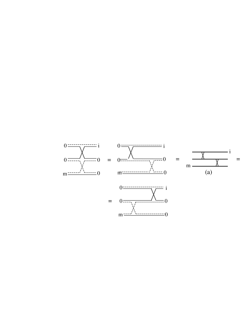
Figure 19: In the case of three excitons, there is only one exchange skeleton in which $m$ and $i$ have no common carrier. If the other excitons are $0$ excitons, we can slide the electron exchange to the left to make appearing two Pauli scatterings with two equal indices on one side. Using figs. 1d and 1e, we then find that this exchange skeleton corresponds to the Pauli diagram (a). A symmetry up-down leads to the Pauli diagram (b). Note that sliding the electron exchange to the right would be of no help.

• For two $0$ excitons, there is one exchange skeleton only (see fig. 19). By “sliding” the carrier exchanges, we get the two equivalent Pauli diagrams shown in fig. 19. They can actually be deduced from one another just by symmetry up/down, which results from $\lambda_{mnij}=\lambda_{nmji}$.

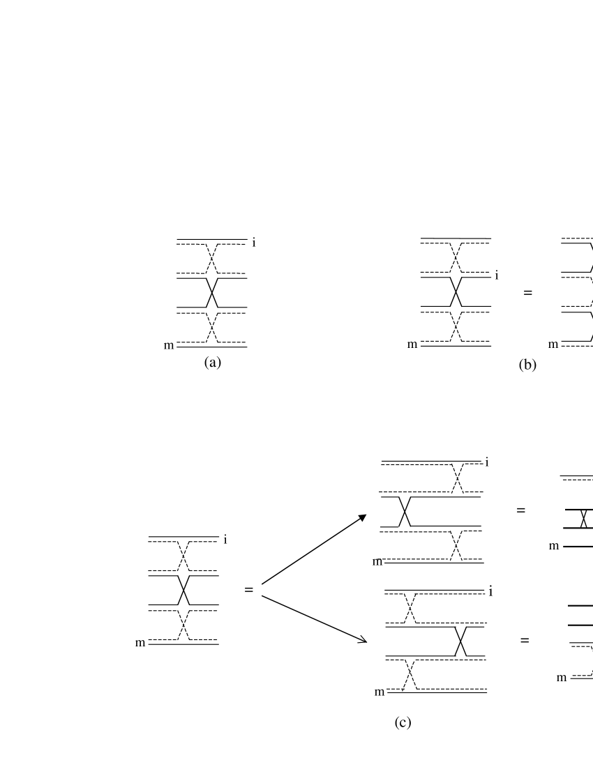
Figure 20: (a,b): In the case of four excitons, there are two different exchange skeletons in which the $m$ and $i$ excitons have no common carrier, as shown in (a) and (b). They correspond to exchange the role played by the electrons and holes. (c): Starting from the exchange skeleton (a), we can slide the carrier exchanges one way or the other, to make appearing Pauli scatterings with two identical excitons $0$ on one side. (d): By combining the two exchange skeletons (a) and (b), we can restore a full $\lambda_{n00i}$ or $\lambda_{m00n}$ to get the two Pauli diagrams (d). They just differ by the order of the zigzags, right, left, right or left, right, left.

• For three $0$ excitons, there are two possible exchange skeletons which are actually related by electron-hole exchange (see figs. 20a and 20b). By sliding the carrier exchanges, we get the two diagrams of fig. 20c, so that, by combining these two exchange skeletons, we find the two Pauli diagrams of fig. 20d.

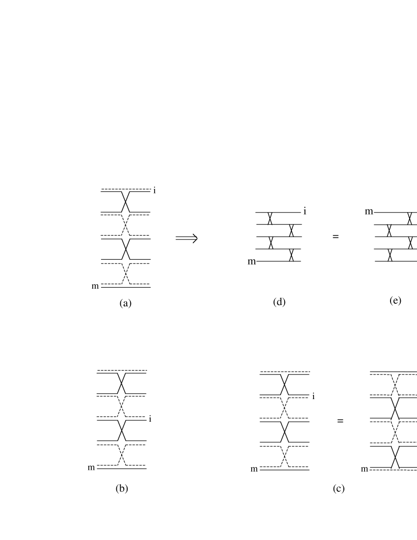
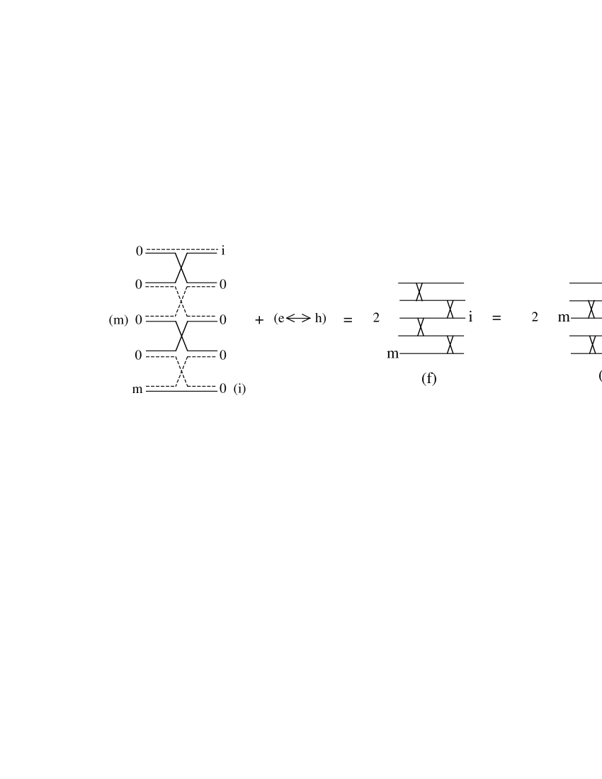
Figure 21: In the case of five excitons, there are three exchange skeletons in which $m$ and have no common carrier. They are shown in figures (a,b,c). By sliding the carrier exchanges of the exchange skeleton (a) with all the other indices equal to $0$, we immediately get the Pauli diagram (d). The diagram (e) follows from an up-down symmetry. If we now add the exchange skeletons (b) and (c) — which just correspond to exchange the roles played by the electrons and holes — and we again slide the carrier exchanges to make appearing Pauli scatterings with two indices on one side equal to $0$, we get the Pauli diagram (f). In the same way, it is possible to obtain the diagram (g) from the same exchange skeletons, by noting that, when all the other indices are equal, it is possible to exchange the positions of the $m$ and $i$ indices in these skeletons.

• In the same way, for four $0$ excitons, there are three possible exchange skeletons, two of them being related by electron-hole exchange (see figs. 21a,21b,21c). By sliding the carrier exchanges, it is again possible to find the Pauli diagrams corresponding to these exchange skeletons as shown in fig. 21.

4.6 Equivalent representations of the diagrams appearing in $A_{N}(m,i)$

By expressing the various Pauli diagrams entering the expansion of $A_{N}(m,i)$ in terms of these exchange skeletons, as shown in figs. (16-21), it is now possible to directly prove their equivalence.

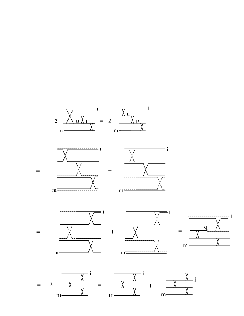
Figure 22: In this figure, we show how to transform the last third order Pauli diagram of $\overline{\overline{\alpha}}_{N}(m,i)$ appearing in fig. 12b, into the two missing zigzag diagrams of fig. 5c which enter $\alpha_{N}(m,i)$, as reproduced at the bottom of this figure. We first use the fact that $\lambda_{n0p0}=\lambda_{0np0}$ to get an equivalent representation of this diagram. We then note that the upper and lower crosses have two identical excitons on one side. By using figs. 1d and 1e for the two upper crosses, and fig. 1a and 1b for the middle cross, we get the two diagrams of the second line of this fig. 22. The diagrams of the next line just follow by sliding the carrier exchanges. In them, we now identify other Pauli scatterings with two identical excitons on one side. These two diagrams can be used to restore the full Pauli scattering $\lambda_{q00i}$. The sum of the last two zigzag diagrams simply results from $\lambda_{q00i}=\lambda_{q0i0}$.

Fig. 22 shows the set of transformations which allows to go from the last third order diagrams of $\overline{\overline{\alpha}}_{N}(m,i)$ to the zigzag Pauli diagrams of $\alpha_{N}(m,i)$, with $i$ at the two upper positions.

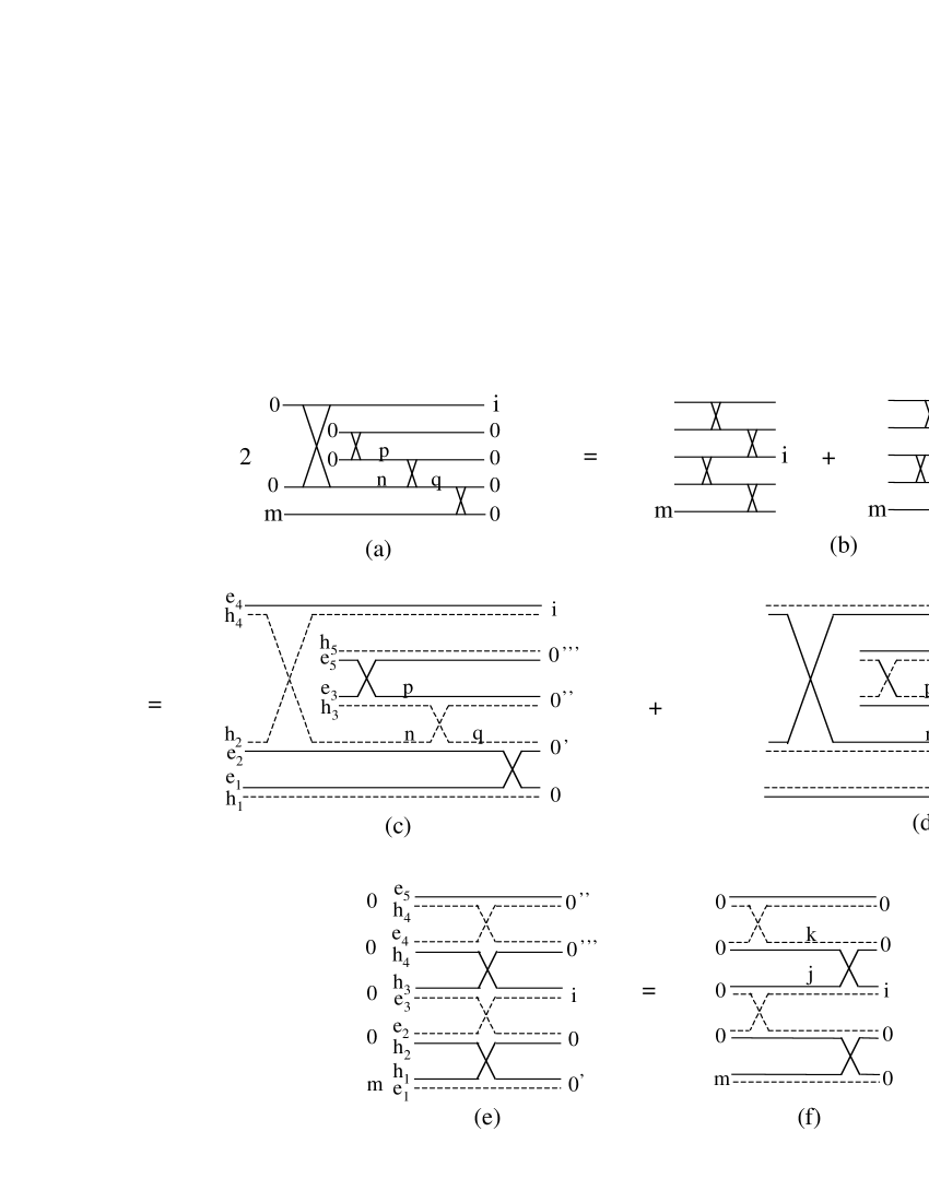
Figure 23: The transformation of the ugly fourth order Pauli diagrams appearing in $\overline{\overline{\alpha}}_{N}(m,i)$ and reproduced in (a), into the two missing zigzag diagrams of $\alpha_{N}(m,i)$ reproduced in (b), is actually quite subtle. In diagram (a), all the Pauli scatterings except $\lambda_{npq0}$ have two $0$ indices on one side. This allows to transform twice the diagram (a) into the sum of diagrams (c) and (d), using figs. 1a,1b and figs. 1d,1e. Diagram (c) is nothing but diagram (e) as easy to see by following the electron and hole lines, in order to check that the excitons with identical electrons or holes are indeed connected. We then slide the carrier exchange to make appearing a Pauli scattering with two excitons $0$ on one side. They are all of this type except the one between $(j,k)$ and $(i,0)$. Using diagram (d), we can restore the full Pauli scattering $\lambda_{jk0i}$. The two diagrams shown in (b) simply result from $\lambda_{jk0i}=\lambda_{jki0}$.

The transformation of the last fourth order diagram for $\overline{\overline{\alpha}}_{N}(m,i)$ into the two missing zigzag diagrams of $\alpha_{N}(m,i)$ is somewhat more subtle. For the interested reader, let us describe in details how this can be done. We have reproduced in fig. 23, the last fourth order diagram of $\overline{\overline{\alpha}}_{N}(m,i)$, as it appears in fig. 12b. We see that all Pauli scatterings have two $0$ indices on one side, except $\lambda_{npq0}$. According to figs. 1a,1b, this $\lambda_{npq0}$ can be represented by the sum of an electron exchange plus a hole exchange between the $(q,0)$ excitons. By continuity, we represent each of the other Pauli scatterings which have two $0$ excitons on one side, either by fig. 1d or by fig. 1e, the choice between these two equivalent representations being driven by avoiding the crossings of electron and hole lines. This leads to the two diagrams of figs. 23b and 23c: They just correspond to exchange the role played by the electrons and the holes.

We now consider one of these two diagrams, namely the one of fig. 23b. Let us call $0$, $0^{\prime}$, $0^{\prime\prime}$ and $0^{\prime\prime\prime}$ the four identical $0$ excitons on the right, in order to recognize them more easily when we will redraw this diagram. To help visualizing this redrawing, we have also given names to the various carriers. It is then straightforward to check that the diagram of fig. 23b corresponds to the samecarrier exchanges as the ones of fig. 23d. Since the diagram of fig. 23c is the same as the one of fig. 23b, with the electrons replaced by holes, we conclude that twice the ugly diagram of fig. 23a is indeed equal to the two missing zigzag diagrams of $\alpha_{N}(m,i)$ reproduced in the top of this figure.

5 Conclusion

In this paper, we have essentially calculated the scalar product of $(N+1)$-exciton states with $N$ of them in the same state $0$. This scalar product is far from trivial due to many-body effects induced by “Pauli scatterings” which originate from the composite nature of excitons. As a result, these scalar products appear as expansions in $\eta=N\mathcal{V}_{X}/\mathcal{V}$, where $\mathcal{V}_{X}$ and $\mathcal{V}$ are the exciton and sample volumes, with possibly some additional factors $N$.

In order to understand the physical origin of these additional $N$’s — which will ultimately differentiate superextensive from regular terms — we have introduced the concept of exciton dressed by a sea of excitons,

$$|\psi_{i}^{(N)}\rangle=\frac{B_{0}^{N}B_{0}^{{\dagger}N}}{\langle v|B_{0}^{N}B_{0}^{{\dagger}N}|v\rangle}\ B_{i}^{\dagger}|v\rangle\ .$$

In the absence of Pauli interaction between the exciton $i$ and the sea of $N$ excitons $0$, the operator in front of $B_{i}^{\dagger}$ reduces to an identity. Due to Pauli interaction, contributions on other exciton states $B_{m\neq i}^{\dagger}|v\rangle$ appear in $|\psi_{i}^{(N)}\rangle$, which originate from possible carrier exchanges between the $i$ exciton and the sea. We moreover find that a bosonic enhancement, which gives rise to an extra factor $N$, — reasonable for the exciton $i=0$, since after all, excitons are not so far from bosons — also exists when the $i$ exciton can be transformed by carrier exchanges into a sea exciton. This happens for any exciton $i$ having the same center of mass momentum as the sea exciton.

In order to understand the carrier exchanges between $N$ excitons, which make the scalar products of $N$-exciton states so tricky, we have introduced “Pauli diagrams”. They read in terms of Pauli scatterings between two excitons. With them, we have shown how to generate a diagrammatic representation of the scalar products of $(N+1)$-exciton states with $N$ of them in the same state $0$, at any order in Pauli interaction.

This diagrammatic representation is actually not unique. Although the one we first give, is nicely simple to memorize, more complicated ones, obtained from other procedures to calculate the same scalar product, are equally good in the sense that they lead to the same correct result.

In order to understand the equivalence between these various Pauli diagrams, we have introduced “exchange skeletons” which correspond to carrier exchanges between more than two excitons. Their appearance in the scalar products of $N$-exciton states is actually quite reasonable because, even if we can calculate these scalar products in terms of Pauli scatterings between two excitons only, Pauli exclusion is originally $N$-body “at once”: When a new exciton is added, its carriers must be in states different from the ones of all the previous excitons. The Pauli scatterings between two excitons generated by our many-body theory for interacting composite bosons, are actually quite convenient to calculate many-body effects between excitons at any order in the interactions. It is however reasonable to find that a set of such Pauli scatterings, which in fact correspond to carrier exchanges between more than two excitons, finally read in terms of these “exchange skeletons”.

The present work is restricted to scalar products of $N$-exciton states in which all of them, except one, are in the same $0$ state. In physical effects involving $N$ excitons, of course enter more complicated scalar products. Such scalar products will be presented in a forthcoming publication. The detailed study presented here, is however all the more useful, because it allows to identify the main characteristics of these scalar products, which are actually present in more complicated situations: As an example, in the case of two dressed excitons $(i,j)$, a bosonic enhancement is found not only for $\mathbf{Q}_{i}$ or $\mathbf{Q}_{j}$ equal to $\mathbf{Q}_{0}$, but also for $\mathbf{Q}_{i}+\mathbf{Q}_{j}=2\mathbf{Q}_{0}$, because these $(i,j)$ excitons can transform themselves into two $0$ excitons by carrier exchanges. The corresponding processes are represented by topologically disconnected Pauli diagrams, and extra factors $N$ appear as a signature of this topology.

REFERENCES

[1] M. Combescot, C. Tanguy, Europhys. Lett. 55, 390 (2001).

[2] M. Combescot, O. Betbeder-Matibet, Europhys. Lett. 58, 87 (2002).

[3] O. Betbeder-Matibet, M. Combescot, Eur. Phys. J. B 27, 505 (2002).

[4] M. Combescot, O. Betbeder-Matibet, Europhys. Lett. 59, 579 (2002).

[5] M. Combescot, X. Leyronas, C. Tanguy, Eur. Phys. J. B 31, 17 (2003).

[6] O. Betbeder-Matibet, M. Combescot, Eur. Phys. J. B 31, 517 (2003).

[7] M. Combescot, O. Betbeder-Matibet, K. Cho, H. Ajiki, Cond-mat/0311387.

[8] A.A. Abrikosov, L.P. Gorkov, I.E. Dzyaloshinski, Methods of quantum field theory in statistical physics, Prentice-hall, inc. Englewood cliffs N.J. (1964).

[9] C. Cohen-Tannoudji, B. Diu, F. Laloë, Mécanique Quantique, Hermann, Paris (1973).

Figure 10: Pauli diagrams for $d_{N}(m,i)$ defined in eq. (55). This $d_{N}(m,i)$ appears instead of $b_{N}(m,i)$ when we write $A_{N}(m,i)$ in terms of $A_{N-2}(n,j)$ and not in terms of $A_{N-2}(n,i)$. As $b_{N}(m,i)$, $d_{N}(m,i)$ is made of disconnected diagrams, with two terms at each order, one with a $\delta_{m0}$ factor, the other with a $\delta_{0i}$ factor.

Figure 14: Various possible representations of the “exchange skeleton” between three excitons. Note that, in all of them, the $m_{1}$ exciton is connected to the $i_{1}$ exciton by an electron line, because these excitons have the same electron, while it is connected to the $i_{2}$ exciton by a hole line, because they have the same hole. And similarly for the other excitons.

Figure 15: A possible carrier exchange between the $(m,n,p)$ and $(i,j,k)$ excitons redrawn using an “exchange skeleton” between three excitons.