Relations between a typical scale and averages
in the breaking of fractal distribution

Abstract

We study distributions which have both fractal and non-fractal scale regions by introducing a typical scale into a scale invariant system. As one of models in which distributions follow power law in the large scale region and deviate further from the power law in the smaller scale region, we employ 2-dim quantum gravity modified by the $R^{2}$ term. As examples of distributions in the real world which have similar property to this model, we consider those of personal income in Japan over latest twenty fiscal years. We find relations between the typical scale and several kinds of averages in this model, and observe that these relations are also valid in recent personal income distributions in Japan with sufficient accuracy. We show the existence of the fiscal years so called bubble term in which the gap has arisen in power law, by observing that the data are away from one of these relations. We confirm, therefore, that the distribution of this model has close similarity to those of personal income. In addition, we can estimate the value of Pareto index and whether a big gap exists in power law by using only these relations. As a result, we point out that the typical scale is an useful concept different from average value and that the distribution function derived in this model is an effective tool to investigate these kinds of distributions.

1 Introduction

Not only in nature but also in social phenomena, various kinds of fractal structures are observed [1]. In a complete self-similar fractal system, similar patterns are repeated in all scales of the system. Even if we gaze a certain part of the system, therefore, we cannot recognize the scale of the part. Fractal is the system without a typical scale and the system is invariant under scale transformation. This is equivalent to that the distribution of the system follows power law.

On the other hand, many fractal structures appear in some restricted scales. In these distributions, the scale exists at which the fractal power law breaks. The study for the breaking of fractal is as important as the study for fractal. Because most elements which constitute such distribution belong to a non-fractal region. There are various distributions which have both fractal and non-fractal scale regions in phenomena which have no relation each other apparently. If these distributions can be understood through some universality which does not depend on the details of an individual system, it may be possible that we can explain those in a unified way by using an appropriate model. For instance, Lévy’s stable distribution [2] and Tsallis’s $q$-Gaussian distribution [3] can explain the distribution which follows power law in the large scale region and deviates from the power law in the other region.

In this paper, we take a following strategy. It is mathematically simple to treat scale free theory. One of the simplest methods to deal with the distribution which has fractal and non-fractal scale regions systematically, therefore, is to introduce a scale into the model, which is originally scale free, by adding an interaction term with a scale:

$$S_{total}=S_{free}+S_{scale}~{}.$$ (1)

Here, $S_{free}$ is the scale free action, $S_{scale}$ is the interaction term with a scale and $S_{total}$ is the total action.

There might be various candidates for $S_{free}$ and $S_{scale}$. As one of kinds of the breaking of fractal, there is the distribution which follows power law in the large scale region and deviates further from the power law in the smaller scale region. We employ 2-dim quantum gravity coupled with conformal matter field as a model which can describe such distribution. We take the standard scale invariant 2-dim action and the $R^{2}$ term with a scale as $S_{free}$ and $S_{scale}$, respectively. Here, the $R^{2}$ term is non-trivial and simplest interaction term with a scale. Because the geometric characters of $S_{free}$ and $S_{scale}$ are known in 2-dim quantum gravity, we can intuitively understand the behavior of fractal and the breaking of fractal.

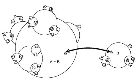
Figure 2: A 2-dim surface is divided into two MINBs.

In this model, the scale free action $S_{free}$ leads the locality that local structure of 2-dim surface does not affect the 2-dim structure away from that place. From this property, it is well known that a typical 2-dim surface has self-similar structure (Fig. 2) [4, 5]. On the other hand, the scale variant action $S_{scale}$ has the effect to let 2-dim surface flat. When this effect cannot be ignored, local structure of 2-dim surface does affect the 2-dim structure away from that place. The locality of 2-dim surface breaks down, therefore, some kind of constraint is imposed on 2-dim surface. As a result, the fractal structure in the small area region breaks down and the typical scale with which fractal collapses is introduced into the system [6, 7].

In Ref. [8], we examined whether the distribution functions obtained in this model could be applied to the distributions in nature or social phenomena. As examples of those which follow power law in the large scale region and deviate further from the power law in the smaller scale region, we considered two distributions of personal income [9, 10, 11] and citation number of scientific papers [12] respectively. We showed that these distributions were fitted fairly well by the distribution derived analytically in this model. We also found that the values of the typical scales were comparable with the average values of the distributions, and concluded that this model worked consistently. Because the quantity which has a scale in the whole distribution does not exist except the average value. This result might show the possibility that we can explain these kinds of distributions universally by using an appropriate model which has similar macroscopic characteristics, not depending on the details of the model. We cannot deny, however, the possibility that the distribution derived in this model are superficially similar to those of personal income and there is no meaning beyond it.

In order to investigate this similarity of distributions more precisely, in this paper, we analyze the personal income distributions in Japan over recent twenty fiscal years. We find relations between the typical scale and several kinds of averages of the distribution in this model. We observe that these relations are also valid with sufficient accuracy in the latest personal income distributions in Japan over two decades years. We also show, in the intelligible form, the existence of the fiscal years in the bubble term, the data of which are thought to be away from one of these relations by the gap arisen in power law. We insist, therefore, that this similarity between the distribution obtained in this model and the personal income distribution is very strict. In addition, even if we do not have detailed distributions in power law, we can guess the value of Pareto index and whether a big gap exists in power law by using only these relations. As a result, we point out that the typical scale is an useful concept, which is different from average value, and the distribution function derived in this model is an effective tool to investigate the distributions which have the similar property to this model.

2 2-dim quantum $R^{2}$ gravity and dynamical triangulation

As mentioned in Sec. 1, we take the standard 2-dim quantum gravity action and the scale variant $R^{2}$ term as a scale free action $S_{free}$ and a scale dependent action $S_{scale}$, respectively;

$$S_{free}(X^{i};g) = \frac{1}{8\pi}\int{\rm d^{2}}x\sqrt{g}g^{\mu\nu}\partial_{\mu}X^{i}\partial_{\nu}X^{i}~{},$$ (2)

$$S_{scale}(X^{i};g) = \frac{w}{64\pi^{2}}\int{\rm d^{2}}x\sqrt{g}\,R^{2}~{}.$$ (3)

Here $X^{i}(i=1,2,\cdots,c)$ are conformal scalar matter fields coupled with gravity, $g_{\mu\nu}(\mu,\nu=0,1)$ is the metric of 2-dim surface, $R$ is the scalar curvature and $w$ is a coupling constant of length dimension $2$. The partition function for fixed area $A$ of 2-dim surface is given by

$$Z(A)=\int\frac{{\cal D}g{\cal D}X}{\rm vol(Diff)}{\rm e}^{-S_{total}(X^{i};g)}~{}\delta(\int d^{2}x\sqrt{g}-A)~{},$$ (4)

where $\rm vol(Diff)$ is the volume of 2-dim diffeomorphisms under which the action and the integration measure ${\cal D}g{\cal D}X$ are invariant. The asymptotic forms of the partition function are evaluated as [6]

$$Z(A) \sim C_{0}~{}A^{\gamma_{0}-3}~{}\exp\biggl{[}-\frac{w}{A}(1-h)^{2}\biggr{]}~{}~{}~{}~{}~{}~{}~{}~{}~{}~{}{\rm for}~{}~{}A\ll w~{},$$ (5)

$$\sim C_{\infty}~{}A^{\gamma_{\infty}-3}~{}~{}~{}~{}~{}~{}~{}~{}~{}~{}~{}~{}~{}~{}~{}~{}~{}~{}~{}~{}~{}~{}~{}~{}~{}~{}~{}~{}~{}~{}~{}~{}~{}{\rm for}~{}~{}A\gg w~{},$$ (6)

where $C_{0}$ and $C_{\infty}$ are proportional constants, and $\gamma_{0}$ and $\gamma_{\infty}$ are constants determined by the central charge $c$ and the number of handles of the 2-dim surface $h$,

$$\gamma_{0}(c,h) = \frac{(c-12)}{6}(1-h)+2~{},$$ (7)

$$\gamma_{\infty}(c,h) = \frac{c-25-\sqrt{(25-c)(1-c)}}{12}(1-h)+2~{}.$$ (8)

Form these expressions of the asymptotic forms (5) and (6), we can observe that fractal power law is broken in the region $A\leq w$. If we take only the standard scale free 2-dim action (2) without the scale variant $R^{2}$ term (3), the theory does not contain the scale $w$, and the partition function follows the fractal power law (6) in all scale regions [4].

In 2-dim quantum gravity, the method is established to observe this phenomenon in numerical simulation. It is known as MINBU analysis [13] in dynamical triangulation (DT) [5]. In DT, 2-dim surface is discretized using small equilateral triangles, where each triangle has the same size. The evaluation of the partition function is performed by replacing the path integral over the metric with the sum over possible triangulations of 2-dim surface. From various evidences, DT is thought to be equivalent to the continuum theory of 2-dim gravity if there are sufficient triangles [14].

A MINBU (minimum-neck baby universe) is defined as a simply connected area region of 2-dim surface whose neck is composed of three sides of triangles, where the neck is closed and non-self intersecting. In MINBU analysis , by dividing a closed 2-dim surface into two MINBUs at a minimum neck (Fig. 2) the statistical average number of finding a MINBU of area $B$ on a closed surface of area $A$, $n_{A}(B)$, can be expressed as

$$n_{A}(B)\sim\frac{B(A-B)Z(B)Z(A-B)}{Z(A)}~{}.$$ (9)

Here we set the area of a triangle $a^{2}=1$ for simplicity. Using the asymptotic forms of the partition functions (5) and (6) in the continuum theory, we obtain the asymptotic expressions of $n_{A}(B)$

$$n_{A}(B) \sim C_{0}~{}A~{}B^{\gamma_{0}-2}\exp\biggl{[}-\frac{w}{B}(1-h)^{2}\biggr{]}\qquad\qquad{\rm for}~{}~{}1\ll B\ll w~{},$$ (10)

$$\sim C_{\infty}~{}A~{}\biggl{[}(1-\frac{B}{A})B\biggl{]}^{\gamma_{\infty}-2}\qquad\qquad\qquad~{}~{}{\rm for}~{}~{}w\ll B<A/2~{}.$$ (11)

These MINBU distributions (10) and (11) keep same properties which partition functions (5) and (6) possess. As for the case $w\ll B$, the asymptotic form (11) follows power law. In this range, even if the model contains the scale $w$, at an area scale much larger than $w$, the surfaces are fractal. On the other hand, as for the case $B\ll w$, the asymptotic form (10) is highly suppressed by the exponential factor $\exp\bigl{[}-\frac{w}{B}(1-h)^{2}\bigr{]}$. In this range, at an area scale much smaller than $w$, the surfaces are affected by the typical length scale $w$. The distribution of smaller MINBUs are, therefore, is apart further from power law. In this paper, we call the distribution (10) and the scale $w$ as Weibull distribution and Weibull scale, respectively.

In DT, the $R^{2}$ term (3) is expressed by

$$\int d^{2}x\sqrt{g}R^{2}\cong\frac{4\pi^{2}}{3}\sum_{i}\frac{(6-q_{i})^{2}}{q_{i}}~{}.$$ (12)

Here $q_{i}$ is the number of triangles sharing the vertex $i$. From Eq. (12), we can recognize that the $R^{2}$ term has the effect to make 2-dim surface flat ($q_{i}=6$) and suppress the possibility that the small MINBUs exist. This effect is parameterized by the coefficient of the $R^{2}$ term. The method to measure MINBU distributions is well known in DT. We can observe the breaking of the fractal by the typical scale in the numerical way.

3 Numerical analysis of DT

The asymptotic forms of MINBU distributions (10) and (11) are analytically obtained in Sec. 2. They can be also confirmed in the simulation of DT for the simple case that 2-dim surface is sphere ($h=0$) and there is no matter field on it ($c=0$) [7]. For example, two simulation results are represented in Figs. 3 and 4, where the total number of triangles is 100,000. We plot MINBU distributions, $n_{A}(B)$ versus $(1-B/A)B$ with a log-log scale for $\beta_{L}=50$ and $100$, which are coefficients of the discretized $R^{2}$ term (12). Here, we can replace $B$ with $(1-B/A)B$ in Eq. (10), because $B\ll w\ll A$. These MINBU distributions can be well explained by the asymptotic formulae (10) and (11) with $\gamma_{0}=0$ and $\gamma_{\infty}=-1/2$ ($h=c=0$). The data fittings for $\beta_{L}=50$ and $100$ are also expressed in Figs. 3 and 4, respectively . From Figs. 3 and 4, we observe that the asymptotic forms (10) and (11) can be applicable to almost all regions of MINBU distributions. These asymptotic representations, therefore, might be used as the approximations of MINBU distributions. In next Sec. 4, we examine this possibility.

4 Approximation of MINBU distributions

In this section, first we postulate the approximation forms of MINBU distributions, and derive relations between Weibull scale $w$ and several kinds of averages by using them. Next, we examine whether these relations are valid in DT simulations. After here, we set $h=0$ for simplicity.

From the asymptotic formulae (10) and (11), we assume that the approximations of MINBU distributions are

$$n_{W}(x) \sim N_{W}~{}x^{\gamma_{0}-2}~{}\exp\biggl{[}-\frac{w}{x}\biggr{]}~{}~{}~{}~{}~{}~{}{\rm for}~{}~{}~{}~{}0\leq x\leq w,$$ (13)

$$n_{P}(x) \sim N_{P}~{}x^{\gamma_{\infty}-2}~{}~{}~{}~{}~{}~{}~{}~{}~{}~{}~{}~{}~{}~{}~{}~{}~{}~{}~{}~{}{\rm for}~{}~{}~{}~{}w\leq x<\infty~{},$$ (14)

where $x=(1-B/A)B$ and $N_{W}$ and $N_{P}$ are normalization constants. Using these forms, we calculate an average of the distribution in power law region $\left\langle(x_{m}\leq)~{}x~{}(\leq x_{M})\right\rangle_{P}$, one in Weibull range $\left\langle x~{}(\leq x_{M})\right\rangle_{W}$ and one in all regions $\left\langle(x_{m}\leq)~{}x\right\rangle_{W+P}$ as follows, respectively:

$$\left\langle(x_{m}\leq)~{}x~{}(\leq x_{M})\right\rangle_{P} \equiv \frac{\int_{x_{m}}^{x_{M}}dx~{}n_{P}(x)~{}x}{\int_{x_{m}}^{x_{M}}dx~{}n_{P}(x)}$$ (15)

$$\sim \frac{1-\gamma_{\infty}}{-\gamma_{\infty}}\left\{1-\left(\frac{x_{m}}{x_{M}}\right)^{-\gamma_{\infty}}\right\}x_{m}~{}~{}~{}{\rm for}~{}~{}~{}\frac{x_{m}}{x_{M}}\ll 1~{},$$

$$\left\langle x~{}(\leq x_{M})\right\rangle_{W} \equiv \frac{\int_{0}^{x_{M}}dx~{}n_{W}(x)~{}x}{\int_{0}^{x_{M}}dx~{}n_{W}(x)}=\frac{\Gamma(-\gamma_{0},\frac{w}{x_{M}})}{\Gamma(1-\gamma_{0},\frac{w}{x_{M}})}w,$$ (16)

$$\left\langle(x_{m}\leq)~{}x\right\rangle_{W+P} \equiv \frac{\int_{x_{m}}^{w}dx~{}n_{W}(x)~{}x+\int_{w}^{\infty}dx~{}n_{P}(x)~{}x}{\int_{x_{m}}^{w}dx~{}n_{W}(x)+\int_{w}^{\infty}dx~{}n_{P}(x)}$$ (17)

$$= \frac{e~{}\Gamma(-\gamma_{0},1)+\frac{1}{-\gamma_{0}}}{e~{}\Gamma(1-\gamma_{0},1)+\frac{1}{1-\gamma_{0}}}w+\frac{1-\gamma_{\infty}}{-\gamma_{\infty}}x_{m}~{}.$$

Here, $\Gamma(z,p)$ is incomplete gamma function defined by $\Gamma(z,p)=\int^{\infty}_{p}dt~{}e^{-t}~{}t^{z-1}$. We used the continuous condition $n_{W}(w)=n_{P}(w)$ to calculate Eq. (17).

In the simulation of DT for the simple case that 2-dim surface is sphere and there is no matter field on it ($\gamma_{0}=0$, $\gamma_{\infty}=-1/2$), these relations can be represented as

$$\left\langle(x_{m}\leq)~{}x\right\rangle_{W+P} \sim \frac{3}{5}\left(e\Gamma(0,1)+2\right)w+3x_{m}~{}~{}~{}~{}~{}~{}~{}~{}~{}~{}~{}~{}~{}~{}~{}~{}~{}~{}~{}~{}~{}{\rm for}~{}~{}~{}\frac{w}{x_{M}}\ll 1$$ (18)

$$\sim 1.56~{}w+3~{}x_{m}~{},$$

$$\left\langle x~{}(\leq x_{M})\right\rangle_{W} \sim e~{}\Gamma(0,1)~{}w-\left\{1-e~{}\Gamma(0,1)\right\}(w-x_{M})~{}~{}~{}{\rm for}~{}~{}~{}1-\frac{x_{M}}{w}\ll 1$$ (19)

$$\sim 0.596~{}w-0.404(w-x_{M})$$

$$= 0.192~{}w+0.404~{}x_{M}~{}.$$ (20)

Analyzing results of DT simulations, we confirm that these relations, which are obtained by using the approximations (13) and (14), are well accurate. First, we express the simulation results and the theoretical line with respect to Eq. (18) in Fig. 5. The horizontal axis indicates Weibull scale and the vertical axis indicates the average. Second, Weibull scale $w$ correlates with $\left\langle x~{}(\leq w)\right\rangle_{W}$ for the case $x_{M}=w$ in Eq. (19). We represent the simulation results and the theoretical line with respect to this correlation $\left\langle x~{}(\leq w)\right\rangle_{W}\sim 0.596~{}w$ in Fig. 6. We also use 100,000 triangles, and plot simulation data for $\beta_{L}=50$, $60$, $70$, $\cdots$, $230$ in these two kinds of simulations. Third, the simulation results and the theoretical line with respect to Eq. (20) are expressed in Fig. 7. We fix $x_{M}=50$ and use the values of $w$ near the $x_{M}$ for $\beta_{L}=98$, $99$, $100$, $101$, $102$.

In every cases, the theoretical lines with respect to Eq. (18), (19) and (20) explain the simulation data with sufficient accuracy. As a result, we recognize Eqs. (13) and (14) as good approximations to calculate the relations between these averages and Weibull scale.

5 Personal Income Distributions

In this section, we point out that the relations in this model are also valid in the personal income distributions interested in Econophysics [15]. We analyze the fiscal years 1980 - 2000.

In Japan, persons who paid the income tax more than 10 million yen are announced publicly as ”high income taxpayers” every year. It is difficult to get the complete data, but we can procure some data from some company. It is possible to estimate the personal income distribution of ”high income taxpayers” by using the method in Ref. [16]. ”The rough distributions of less than 50 million yen income earners” are also released by the National Tax Administration Agency in Japan. These are comparatively easy to get and we can download latest data from web page [17]. We can obtain the distribution of all income earners combining these two kinds of data.

In Ref. [8], we examined whether the distributions derived in this model could be applicable to the personal income distributions in 1997 and 1998 Japan in which we procured ”high income taxpayers” data from Ref. [18]. We observed that $\gamma_{\infty}-2=-3$ in the power law region (11), then we decided that $\gamma_{0}-2=-7/3$ in Weibull region (10). These parameters are realized by setting that $c=-2$ and $h=0$. We showed that the personal income distributions were also fitted fairly well by the distributions (10) and (11), and the typical scales could be read consistently (Figs. 8 and 9). In these Figs, the horizontal axis indicates the income $x$ in units of 10 thousand yen and the vertical axis indicates the number density of persons per a period of 100 thousand yen.

Recently, in Ref. [19], it is reported that the value $\gamma_{\infty}-2$ is almost $-3$ (Pareto Index $\alpha=2$) in 1987 - 2000 Japan. Combining this report and ”the rough distribution” released by the National Tax Administration Agency, we can calculate Weibull scales in these fiscal years in a same mannar in 1997 or 1998 Japan. We can also estimate income average values by using the data with respect to the sum of income and the total number of income earners which the National Tax Administration Agency has also announced (Fig. 10). We examine whether the relations between Weibull scale and several kinds of averages, which is verified in Sec. 4, are valid in these data of the personal income distributions in recent Japan. In order to consider fiscal years before, in and after bubble term in Japan continuously, we analyze the fiscal years 1980 - 2000 assuming that the value $\gamma_{\infty}-2$ is almost $-3$ in 1980 - 1986 likely in 1987 - 2000.

Using the approximate distribution functions (13) and (14), from Eqs. (16) and (17) for the case that $\gamma_{0}=-1/3$ and $\gamma_{\infty}=-1$ we obtain the average in all regions $\left\langle(x_{m}\leq)~{}x\right\rangle_{W+P}$ and one in Weibull range $\left\langle x~{}(\leq x_{M})\right\rangle_{W}$ as follows, respectively:

$$\left\langle(x_{m}\leq)~{}x\right\rangle_{W+P} \sim 0.980~{}w+2~{}x_{m}~{},$$ (21)

$$\left\langle x~{}(\leq x_{M})\right\rangle_{W} = \frac{\Gamma(\frac{1}{3},\frac{w}{x_{M}})}{\Gamma(\frac{4}{3},\frac{w}{x_{M}})}~{}w$$ (22)

$$\sim 0.566~{}w-0.353(w-x_{M})~{}~{}~{}{\rm for}~{}~{}~{}1-\frac{x_{M}}{w}\ll 1$$

$$= 0.213~{}w+0.353~{}x_{M}~{}.$$ (23)

We show average values in whole distribution and Weibull scales, and also express the theoretical lines (21) in Fig. 11. Because classification of data in 1980 - 1988 is different from one in 1989 - 2000, there are two theoretical lines corresponding to two different values of $x_{m}$. These values are represented in units of 10 thousand yen. It turns out that the data of 1980 - 1986 and 1992 - 2000 fiscal years agree with each theoretical line respectively, and that those of 1987 - 1991 fiscal years disagree with either. In Ref. [19] Cit is also reported that the gap, which cannot be disregarded, in power law has arisen in the 1987 - 1991 fiscal years, so called bubble term. Error bars in Fig. 1 in Ref. [19] indicate the gaps. Our model presupposes the power law in the large scale region. The distribution function in this model, therefore, cannot be applicable to the distributions in this term strictly and the relation between average values in whole distribution and Weibull scales (21) is not maintained. Moreover, from the result that this relation keeps in 1980 - 1986, we guess that there are not big gaps in the power law and the value $\gamma_{\infty}-2$ is almost $-3$ in this term.

On the other hand, we cannot examine the relation $\left\langle x~{}(\leq w)\right\rangle_{W}\sim 0.566~{}w$ in Eq. (22) for the case $x_{M}=w$, because we have no data in which the value $x_{M}$ can be finely moved according to the change of the value of $w$. It is possible, however, to examine the relation (23) between Weibull scale $w$ and $\left\langle x~{}(\leq x_{M})\right\rangle_{W}$ by fixing the value of $x_{M}$. In Fig. 12, the relation (23) for the case $x_{M}=400$ is confirmed in 1988 - 1997, 1999, 2000 fiscal years where Weibull scales are almost 4 million yen. In Fig. 13, the relation (23) for the case $x_{M}=300$ is also confirmed in 1980 - 1988 fiscal years where Weibull scales are almost 3 million yen. The data in 1987 - 1991 fiscal years, where the gap has arisen in power law, are not away from this relation (23). It can be understood that the distribution in power law does not have great influence on the average in Weibull region.

We find that the relation (21) is also valid in the distributions of personal income. This means that the position of the typical scale in the whole distribution in our model is very similar to the position in the personal income distributions. We also find that the relation (23) keeps in the personal income distributions. This means that the two kinds of distributions in the region where variables are smaller than the typical scale is also very alike. From these observations, we conclude that there is high similarity between the distribution derived in our model and those of personal income in latest Japan, and that our distribution function can be applicable to the personal income distribution.

6 Summary and discussion

We studied the breaking of fractal distribution by introducing a typical scale into a scale invariant system in which the distribution is fractal. We employed 2-dim quantum gravity modified by the $R^{2}$ term as the model which can describe the distribution which follows power law in the large scale region and deviates further from the power law in the smaller scale region. We concentrated ourselves on considering the personal income distribution which has similar property to this model in the real world. In Ref. [8], we only pointed out that the distribution derived in this model can fit those of personal income in 1997 and 1998 Japan. In this paper, we found relations between the typical scale and several kinds of averages of the distribution in this model. We observe that these relations are also valid with sufficient accuracy in the personal income distributions in 1980 - 2000 Japan. We also showed that the data in 1987 - 1991 fiscal years are apart from one of these relations. This reason can be thought to be that gaps have arisen in the power law in these years. This phenomenon is reported in Ref. [19]. We also estimated that there are not big gaps in the power law in 1980 - 1986 fiscal years and the values of Pareto index in these years are almost $2$. This is concluded by the agreement of this relation with data in these years. In this analysis, we do not need the details of the distribution of high income earners. As a result, we consider that the typical scale is an useful concept and that the distribution function in this model is an effective tool to investigate the distributions which have the similar property to this model.

We do not understand that this coincidence of the distributions can be thought to be an universal property. In other words, we cannot refer to any physical connection between 2-dim $R^{2}$ gravity and personal income. The following speculations, however, might give some insight. Fractal is observed in the system described by only independent variables. This is realized in 2-dim gravity. This situation is also expected to be realized in free competition which leads the distribution of high income earners. On the other hand, the breaking of fractal is observed in the system with some kind of constraint. This is realized in 2-dim gravity with the $R^{2}$ term in which this constraint is induced by the interaction with 2-dim surface. We expect that there is also some kind of interaction in middle income earners [20]. These way of thinking might be clear by investigating the company’s income distributions which have more informations than those of personal income.

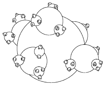
Figure 1: A fractal 2-dim surface.

Figure 3: The simulation data and the fitting of $\beta_{L}=50$.

Figure 4: The simulation data and the fitting of $\beta_{L}=100$.

Figure 5: The relation between Weibull scales $w$ and average values of the whole distribution $\left\langle(x_{m}\leq)~{}x\right\rangle_{W+P}$ in DT simulations.

Figure 6: The relation between Weibull scales $w$ and average values below the Weibull scale $\left\langle x~{}(\leq w)\right\rangle_{W}$ in DT simulations.

Figure 7: The relation between Weibull scales $w$ and average values below MINBU area $50$ $\left\langle x~{}(\leq 50)\right\rangle_{W}$ in DT simulations.

Figure 8: The personal income distribution and the data fitting in 1997 Japan.

Figure 9: The personal income distribution and the data fitting in 1998 Japan.

Figure 10: Weibull scales and average values of the personal income in 1980 - 2000 Japan.

Figure 11: The relation between Weibull scales $w$ and average values of the whole personal income $\left\langle(x_{m}\leq)~{}x\right\rangle_{W+P}$ in 1980 - 2000 Japan.

Figure 12: The relation between Weibull scales $w$ and average values of the personal income below $4$ million yen $\left\langle x~{}(\leq 400)\right\rangle_{W}$ in 1988 - 1997, 1999, 2000 Japan.

Figure 13: The relation between Weibull scales $w$ and average values of the personal income below $3$ million yen $\left\langle x~{}(\leq 300)\right\rangle_{W}$ in 1980 - 1988 Japan.

References

- [1] B.P. Mandelbrot, The Fractal Geometry of Nature, Freeman, San Francisco, 1982.
- [2] P. Lévy, Calcul des probabilités, Gauthier-Villas, Paris, 1925.
-
[3]
C. Tsallis, J. Stat. Phys. 52 (1998) 479;
E.M.F. Curado and C. Tsallis, J. Phys. A: Math. Gen. 24 (1991) L69;
E.M.F. Curado and C. Tsallis, J. Phys. A: Math. Gen. 24 (1991) 3187 (corrigendum);
E.M.F. Curado and C. Tsallis, J. Phys. A: Math. Gen. 25 (1192) 1019 (corrigendum);
C. Tsallis, R.S. Mendes and A.R. Plastino, Physica A 261 (1998) 534. -
[4]
E. Brezin, C. Itzykson, G. Parisi and J.B. Zuber, Commun. Math. Phys. 59 (1978) 35;
F. David, Mod. Phys. Lett. A3 (1988) 1651;
J. Distler and H. Kawai, Nucl. Phys. B321 (1989) 509;
V.G. Knizhinik, A.M. Polyakov and A.B. Zamolodchikov, Mod. Phys. Lett. A3 (1988) 819. -
[5]
V.A. Kazakov, I.K. Kostov and A.A. Migdal, Phys. Rev. Lett. 66 (1991) 2051;
J. Ambjorn, B. Durhuus and J. Frohlich, Nucl. Phys. B257 (1985) 433;
F. David, Nucl. Phys. B 257 (1985) 543. - [6] H. Kawai and R. Nakayama, Phys. Lett. B306 (1993) 224.
-
[7]
S. Ichinose, N. Tsuda and T. Yukawa, Int. J. Mod. Phys. A12 (1997) 757;
A. Fujitsu, N. Tsuda and T. Yukawa, Int. J. Mod. Phys. A13 (1998) 583. - [8] M. Anazawa, A. Ishikawa, T. Suzuki and M. Tomoyose, Phsica A335 (2004) 616.
- [9] V. Pareto, Cours d’Economique Politique, Macmillan, London, 1897.
- [10] R. Gibrat, Les inegalits economiques, Paris, Sirey, 1931.
-
[11]
W.W. Badger, Mathematical models as a tool for the social science, ed. B. J. West,
New York, Gordon and Breach, 1980, pp. 87;
E.W. Montrll and M.F. Shlesinger, J. Stat. Phys. 32 (1983) 209. - [12] S. Render, Eur. Phys. J. B4 (1998) 131.
-
[13]
S. Jain and S.D. Mathur, Phys. Lett. B286 (1992) 239;
J. Ambijorn, S. Jain and G. Thorleifsson, Phys. Lett. B307 (1993) 34. -
[14]
E. Brezin and V. Kazakov, Phys. Lett. B236 (1990) 144;
M. Douglas and S. Shenker, Nucl. Phys. B335 (1990) 635;
D.J. Gross and A. Migdal, Phys. Rev. Lett. 64 (1990) 127;
M. Douglas, Phys. Lett. B238 (1990) 176;
M. Fukuma, H. Kawai and R. Nakayama, Int. J. Mod. Phys. A6 (1991) 1385;
M. Fukuma, H. Kawai and R. Nakayama, Commun. Math. Phys. 143, 371 (1992);
M. Fukuma, H. Kawai and R. Nakayama, Commun. Math. Phys. 148 (1992) 101;
R. Dijkgraaf, E. Verlinde and H. Verlinde, Nucl. Phys. B348 (1991) 435;
A. Jevicki and T. Yoneya, Mod. Phys. Lett. A5 (1990) 1615;
P. Ginsparg, M. Goulian, M. Plesser and J. Zinn-Justin, Nucl. Phys. B342 (1990) 539;
T. Yoneya, Commun. Math. Phys. 144 (1992) 623; Int. J. Mod. Phys. A7 (1992) 4015;
J. Goeree, Nucl. Phys. B358 (1991) 737. - [15] R.N. Mategna and H.E. Stanley, An Introduction to Econophysics, (Cambrige Univ. Press, U. K., 2000).
-
[16]
H. Aoyama, W. Souma, Y. Nagahara, H.P. Okazaki, H. Takayasu and
M. Takayasu,
Fractals 8, 293 (2000);
W. Souma, Fractals 9, 463 (2001). - [17] The Japanese Tax Administration, http://www.nta.go.jp.
- [18] General Legal Security, Inc., http://chouja.houmu.co.jp.
- [19] Y. Fujiwara, W. Souma, H. Aoyama, T. Kaizoji and M. Aoki, Physica A321 (2003) 598.
- [20] W. Souma, Y. Fujiwara and H. Aoyama, cond-mat/0108482, KUCP0189.