Investigation of the incremental response of soils using a discrete element model

Abstract

The incremental stress-strain relation of dense packings of polygons is investigated here by using molecular dynamics simulations. The comparison of the simulation results to the continuous theories is performed using explicit expressions for the averaged stress and strain over a representative volume element. The discussion of the incremental response raises two important questions of soil deformation: Is the incrementally non-linear theory appropriate to describe the soil mechanical response? Does a purely elastic regime exists in the deformation of granular materials?. In both cases our answer will be ”no”. The question of stability is also discussed in terms of the Hill condition of stability for non-associated materials.

I Introduction

For many years the study of the mechanical behavior of soils was developed in the framework of linear elasticity [1] and the Mohr-Coulomb failure criterion [2] However, since the start of the development of the non-linear constitutive relations in 1968 [3], a great variety of constitutive models describing different aspects of soils have been proposed [4]. A crucial question has been brought forward: What it the most appropriate constitutive model to interpret the experimental result, or to implement a finite element code? Or more precisely, why is the constitutive relation I am using better than that one of the fellow next lab?

In the last years, the discrete element approach has been used as a tool to investigate the mechanical response of soils at the grain level [5]. Several average procedures have been proposed to define the stress [6, 7, 8] and the strain tensor [9, 10] in terms of the contact forces and displacements at the individual grains. These methods have been used to perform a direct calculation of the incremental stress-strain relation of assemblies of disks [11] and spheres [12], without any a-priori hypothesis about the constitutive relation. Some of the results lead to the conclusion that the non-associated theory of elasto-plasticity is sufficient to describe the observed incremental behavior [11]. However, some recent investigations using three-dimensional loading paths of complex loading histories seem to contradict these results [13, 12]. Since the simple spherical geometries of the grains overestimate the role of rotations in realistic soils [13], it is interesting to evaluate the incremental response using arbitrarily shaped particles.

In this paper we investigate the incremental response in the quasi-static deformation of dense assemblies of polygonal particles. The comparison of the numerical simulations with the constitutive theories is performed by introducing the concept of Representative Volume Element (RVE). This volume is chosen the smear out the strong fluctuations of the stress and the deformation in the granular assembly. In the averaging, each grain is regarded as a piece of continuum. By supposing that the stress and the strain of the grain are concentrated at the small regions of the contacts, we obtain expressions for the averaged stress and strain over the RVE, in terms of the contact forces, and the individual displacements and rotations of the grains. The details of this homogenization method are presented in Sec. II. A short review of the incremental, rate-independent stress-strain models is presented in Sec. III. We make special emphasis in the classical Drucker-Prager elasto-plastic models and the recently elaborated theory of hypoplasticity. The details of the particle model are presented in Sec. IV. The interparticle forces include elasticity, viscous damping and friction with the possibility of slip. The system is driven by applying stress controlled tests on a rectangular framework consisting of four walls. Some loading programs were implemented in Sec. V, in order to lead to four basic question on the incremental response of soils: 1) The existence of tensorial zones in the incremental response, 2) the validity of the superposition principle and 3) the existence of a finite elastic regime and 4) the question of stability according to the Hill condition.

II Homogenization

The aim of this section is to calculate the macro-mechanical quantities, the stress and strain tensors, from micro-mechanical variables of the granular assembly such as contact forces, rotations and displacements of individual grains.

A particular feature of granular materials is that both the stress and the deformation gradient are very concentrated in small regions around the contacts between the grains, so that they vary strongly on short distances. The standard homogenization procedure smears out these fluctuations by averaging these quantities over a RVE. The diameter $d$ of the RVE must be such that $\delta\ll d\ll D$, where $\delta$ is the characteristic diameter of the particles and $D$ is the characteristic length of the continuous variables.

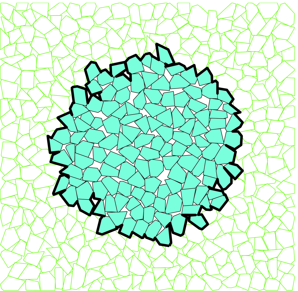
FIG. 1.: Representative volume element (RVE).

We use here this procedure to obtain the averages of the stress and the strain tensors over a RVE in granular materials, which will allow us to compare the molecular dynamics simulations to the constitutive theories. We regard stress and strain to be continuously distributed through the grains, but concentrated at the contacts. It is important to comment that this averaging procedure would not be appropriate to describe the structure of the chain forces or the shear band because typical variations of the stress corresponds to few particle diameters. Different averaging procedures using coarse-grained functions [8], or cutting the space in slide-shaped areas [14, 10], can deal with the question of how one can perform averages, and at the same time maintain these features.

We will calculate the averages around a point $\vec{x}_{0}$ of the granular sample taking a RVE calculated as follows: at the initial configuration, we select the grains whose center of mass are less than $d$ from $\vec{x}_{0}$. Then the RVE is taken as the volume $V$ enclosed by the initial configuration of the grains. See Fig. 1. The diameter $d$ is taken, so that the averaged quantities are not sensible to the increase of the diameter by one particle diameter.

A Micro-mechanical stress

The Cauchy stress tensor is defined using the force acting on an area element situated on or within the grains. Let $\vec{f}$ be the force applied on a surface element $a$ whose normal unit vector is $\vec{n}$. Then the stress is defined as the tensor satisfying [1]:

$$\sigma_{kj}n_{k}=lim_{a\to 0}{f_{j}/a},$$ (1)

where the Einstein summation convention is used. In absence of body forces, the equilibrium equations in every volume element lead to [1]:

$$\partial\sigma_{ij}/\partial x_{i}=0.$$ (2)

We are going to calculate the average of the stress tensor $\bar{\sigma}$ over the RVE:

$$\bar{\sigma}=\frac{1}{V}\int_{V}{\sigma dV}.$$ (3)

Since there is no stress in the voids of the granular media, the averaged stress can be written as the sum of integrals taken over the particles

$$\bar{\sigma}=\frac{1}{V}\sum^{N}_{\alpha=1}{\int_{V_{\alpha}}{\sigma_{ij}dV}},$$ (4)

where $V_{\alpha}$ is the volume of the particle $\alpha$ and $N$ is the number of particles of the RVE. Using the identity

$$\frac{\partial(x_{i}\sigma_{kj})}{\partial x_{k}}=x_{i}\frac{\partial\sigma_{kj}}{\partial x_{k}}+\sigma_{ij},$$ (5)

Eq. (2), and the Gauss theorem, Eq. (4) leads to

$$\bar{\sigma}_{ij}=\frac{1}{V}\sum_{\alpha}{\int_{V_{\alpha}}{\frac{\partial(x_{i}\sigma_{kj})}{\partial x_{k}}dV}}=\frac{1}{V}\sum_{\alpha}{\int_{\partial V_{\alpha}}{x_{i}\sigma_{kj}n_{k}da}}.$$ (6)

The right hand side is the sum over the surface integrals of each grain. $\partial V_{\alpha}$ represents the surface of the grain $\alpha$ and $\vec{n}$ is the unit normal vector to the surface element $da$.

An important feature of granular materials is that the stress acting on each grain boundary is concentrated in the small regions near to the contact points. Then we can use the definition given in Eq. (1) to express this stress on particle $\alpha$ in terms of the contact forces by introducing Dirac delta functions:

$$\sigma_{kj}n_{k}=\sum^{N_{\alpha}}_{\beta=1}{f^{\alpha\beta}_{j}\delta(\vec{x}-\vec{x}^{\alpha\beta})},$$ (7)

where $\vec{x}^{\alpha\beta}$ and $\vec{f}^{\alpha\beta}$ are the position and the force at the contact $\beta$, and $N_{\alpha}$ is the number of contacts of the particle $\alpha$. Replacing Eq. (7) into Eq. (6), we obtain

$$\bar{\sigma}_{ij}=\frac{1}{V}\sum_{\alpha\beta}{x^{\alpha\beta}_{i}}f^{\alpha\beta}_{j}.$$ (8)

Now we decompose $\vec{x}^{\alpha\beta}=\vec{x}^{\alpha}+\vec{\ell}^{\alpha\beta}$ where $\vec{x}^{\alpha}$ is the position of the center of mass and $\vec{\ell}^{\alpha\beta}$ is the branch vector, connecting the center of mass of the particle to the point of application of the contact force. Imposing this decomposition in Eq. (8), and using the equilibrium equations at each particle $\sum_{\beta}{\vec{f}^{\alpha\beta}}=0$ we have

$$\bar{\sigma}_{ij}=\frac{1}{V}\sum_{\alpha\beta}{\ell^{\alpha\beta}_{i}}f^{\alpha\beta}_{j}.$$ (9)

From the equilibrium equations of the torques $\sum_{\beta}(\ell^{\alpha\beta}_{i}f^{\alpha\beta}_{j}-\ell^{\alpha\beta}_{j}f^{\alpha\beta}_{i})=0$ one obtains that this tensor is symmetric, i. e.,

$$\bar{\sigma}_{ij}-\bar{\sigma}_{ji}=0.$$ (10)

Then, the eigenvalues of this matrix are always real. This property leads to some simplifications, as we will see later.

B Micro-mechanical strain

In elasticity theory, the strain tensor is defined as the symmetric part of the average of the displacement gradient with respect to the equilibrium configuration of the assembly. Using the law of conservation of energy, one can define the stress-strain relation in this theory [1]. In granular materials, it is not possible to define the strain in this sense, because any loading involves a certain amount of plastic deformation at the contacts, so that it is not possible to define the initial reference state to calculate the strain. Nevertheless, one can define a strain tensor in the incremental sense. This is defined as the average of the displacement tensor taken from the deformation during a certain time interval.

At the micro-mechanical level, the deformation of the granular materials is given by a displacement field $\vec{u}=\vec{r^{\prime}}-\vec{r}$ at each point of the assembly. Here $\vec{r}$ and $\vec{r^{\prime}}$ are the positions of a material point before and after deformation. The average of the strain and rotational tensors are defined as:

$$\bar{\epsilon}=\frac{1}{2}(F+F^{T}),$$ (11)

$$\bar{\omega}=\frac{1}{2}(F-F^{T}).$$ (12)

Here $F^{T}$ is the transpose of the deformation gradient $F$, which is defined as

$$F_{ij}=\frac{1}{V}\int_{V}{\frac{\partial u_{i}}{\partial x_{j}}dV}.$$ (13)

Using the Gauss theorem, we transform it into an integral over the surface of the RVE

$$F_{ij}=\frac{1}{V}\int_{\partial V}{u_{i}n_{j}da},$$ (14)

where $\partial V$ is the boundary of the volume element. We express this as the sum over the boundary particles of the RVE

$$F_{ij}=\frac{1}{V}\sum^{N_{b}}_{\alpha=1}\int_{\partial V_{\alpha}}{u_{i}n_{j}da},$$ (15)

where $N_{b}$ is the number of boundary particles. To go further it is convenient to make some approximations. First, the displacements of the grains during deformation can be considered rigid except for the small deformations near to the contact that can be neglected. Then, if the displacements are small in comparison to the size of the particles, we can write the displacement of the material points inside of particle $\alpha$ as:

$$u_{i}(\vec{x})\approx\Delta x^{\alpha}_{i}+e_{ijk}\Delta\phi^{\alpha}_{j}(x_{k}-x^{\alpha}_{k}),$$ (16)

where $\Delta\vec{x}^{\alpha}$, $\Delta\vec{\phi}^{\alpha}$ and $\vec{x^{\alpha}}$ are displacement, rotation and center of mass of the particle $\alpha$ which contains the material point $\vec{x}$, and $e_{ijk}$ is the anti-symmetric unit tensor. Setting a parameterization for each surface of the boundary grains over the RVE, the deformation gradient can be explicitly calculated in terms of grain rotations and displacements by replacing Eq. (16) in Eq. (15).

In the particular case of a bidimensional assembly of polygons, the boundary of the RVE is given by a graph $\{\vec{x_{1}}..\vec{x_{2}},...,\vec{x}_{N_{b}+1}=\vec{x_{1}}\}$ consisting of all the edges belonging to the external contour of the RVE, as shown in Fig. 1. In this case, Eq. (15) can be transformed as a sum of integrals over the segments of this contour.

$$F_{ij}=\frac{1}{V}\sum^{N_{b}}_{\beta=1}{\int^{x_{\beta+1}}_{x_{\beta}}{[\Delta x^{\beta}_{i}+e_{ik}\Delta\phi^{\beta}(x_{k}-x^{\beta}_{k})]n^{\beta}_{j}ds}},$$ (17)

where $e_{ik}\equiv e_{i3k}$ and the unit vector $\vec{n}^{\beta}$ is perpendicular to the segment $\overrightarrow{x^{\beta}x^{\beta+1}}$. Here $\beta$ corresponds to the index of the boundary segment. $\Delta\vec{x}^{\beta}$, $\Delta\vec{\phi}^{\beta}$ and $\vec{x^{\beta}}$ are displacement, rotation and center of mass of the particle which contains this segment. Finally, by using the parameterization $\vec{x}=\vec{x}^{\beta}+s(\vec{x}^{\beta+1}-\vec{x}^{\beta})$, where $(0<s<1)$, we can integrate Eq. (17) to obtain

$$F_{ij}=\frac{1}{V}\sum_{\beta}{(\Delta x^{\beta}_{i}+e_{ik}\Delta\phi^{\beta}\ell^{\beta}_{k})N^{\beta}_{j}},$$ (18)

where $N^{\beta}_{j}=e_{j,k}(x^{\beta+1}_{k}-x^{\beta}_{k})$ and $\vec{\ell}=(\vec{x}^{\beta+1}-\vec{x}^{\beta})/2-\vec{x}^{\alpha}$. The stress tensor can be calculated taking the symmetric part of this tensor using Eq. (11). Contrary to the strain tensor calculated for spherical particles [15], the individual rotation of the particles appears in the calculation of this tensor. This is given by the fact that for non-spherical particles the branch vector is not perpendicular to the contact normal vector, so that $e_{ik}\ell^{\beta}_{k}N^{\beta}_{j}\neq 0$.

III Incremental theory

Since the stress and the strain tensor are symmetric, it is advantageous to simplify the notation by defining these quantities as six-dimensional vectors:

$$\tilde{\sigma}=\left[\begin{array}[]{c}\bar{\sigma}_{11}\\ \bar{\sigma}_{22}\\ \bar{\sigma}_{33}\\ \sqrt{2}\bar{\sigma}_{23}\\ \sqrt{2}\bar{\sigma}_{31}\\ \sqrt{2}\bar{\sigma}_{13}\\ \end{array}\right],~{}~{}~{}and~{}~{}~{}~{}\tilde{\epsilon}=\left[\begin{array}[]{c}\bar{\epsilon}_{11}\\ \bar{\epsilon}_{22}\\ \bar{\epsilon}_{33}\\ \sqrt{2}\bar{\epsilon}_{23}\\ \sqrt{2}\bar{\epsilon}_{31}\\ \sqrt{2}\bar{\epsilon}_{13}\\ \end{array}\right]$$ (19)

The coefficient$\sqrt{2}$ allows us to preserve the metric in this transformation: $\tilde{\sigma}_{k}\tilde{\sigma}_{k}=\bar{\sigma}_{ij}\bar{\sigma}_{ij}$ . The relation between these two vectors will be established in the general context of the rate-independent incremental constitutive relations. We will focus on two particular theoretical developments: the theory of hypoplasticity and the elasto-plastic models. The similarities and differences of both formulations are presented in the framework of the incremental theory as follows.

A General framework

In principle, the mechanical response of granular materials can be described by a functional dependence of the stress $\tilde{\sigma}(t)$ at time $t$ on the strain history $\{\tilde{\epsilon}(t^{\prime})\}_{0<t^{\prime}<t}$. However, the mathematical description of this dependence turns out to be very complicated due to the non-linearity and irreversible behavior of these materials. An incremental relation, relating the incremental stress $d\tilde{\sigma}(t)=\sigma^{\prime}(t)dt$ with the incremental strain $d\tilde{\epsilon}(t)=\epsilon^{\prime}(t)dt$ and some internal variables $\chi$ accounting for the deformation history, enables us to avoid these mathematical difficulties [16]. This incremental scheme is also useful to solve geotechnical problems, since the finite element codes require that the constitutive relation be expressed incrementally.

Due to the large number of existing incremental relations, the necessity of a unified theoretical framework has been pointed out as an essential necessity to classify all the existing models [17] In general, the incremental stress is related to the incremental strain by the following function:

$${\cal F}_{\chi}(d\tilde{\epsilon},d\tilde{\sigma},dt).$$ (20)

Let’s look at the special case where there is no rate dependence in the constitutive relation. This means that this relation is not influenced by the time required during any loading tests, as corresponds to the quasi-static approximation. In this case ${\cal F}$ is invariant with respect to $dt$, and Eq. (20) can be reduced to:

$$d\tilde{\epsilon}={\cal G}_{\chi}(d\tilde{\sigma})$$ (21)

In particular, the rate-independent condition implies that multiplying the loading time by a scalar $\lambda$ does not affect the incremental stress-strain relation:

$$\forall\lambda,~{}~{}~{}{\cal G}_{\chi}(\lambda d\tilde{\sigma})=\lambda{\cal G}_{\chi}(d\tilde{\sigma})$$ (22)

This equation means that ${\cal G}_{\chi}$ is an homogeneous function of degree one. In this case, the application of the Euler identity shows that Eq. (21) leads to

$$d\tilde{\epsilon}=M_{\chi}(\hat{\sigma})d\tilde{\sigma},$$ (23)

where $M_{\chi}=\partial{\cal G}_{\chi}/\partial(d\tilde{\sigma})$ and $\hat{\sigma}$ is the unitary vector defining the direction of the incremental stress

$$\hat{\sigma}=\frac{d\tilde{\sigma}}{|d\tilde{\sigma}|}.$$ (24)

Eq. (23) represents the general expression for the rate-independent constitutive relation. In order to determine the dependence of $M$ on $\hat{\sigma}$, one can either perform experiments by taking different loading directions, or postulate explicit expressions based on a theoretical framework. The first approach will be considered in the next section, and the discussion about some existing theoretical models will be presented as follows.

B Elasto-plastic models

The classical theory of elasto-plasticity has been established by Drucker and Prager in the context if metal plasticity [18]. Some extensions have been developed to describe soils, clays, rocks, concrete, etc. [2, 19]. Here we present a short review of these developments in soil mechanics.

When a granular sample subjected to a confining pressure is loaded in the axial direction, it displays a typical stress-strain response as shown in the left part of Fig. 2. A continuous decrease of the stiffness (i.e. the slope of the stress-strain curve) is observed during the loading. If the sample is unloaded, an abrupt increase in the stiffness is observed, leaving an irreversible deformation. One observes that if the stress is changed around some region below $\sigma_{A}$, which is called the yield point, the deformation is almost linear and reversible. The first postulate of the elasto-plastic theory establishes a stress region immediately below the yield point where only elastic deformations are possible.

Postulate 1: For each stage of loading there exists a yield surface, which encloses a finite region in the stress space where only reversible deformations are possible.

The simple Mohr-Coulomb model assumes that the onset of plastic deformation occurs at failure [2]. However, it has been experimentally shown that plastic deformation develops before failure [20]. In order to provide a consistent description of these experimental results with the elasto-plastic theory, it is necessary to suppose that the yield function changes with the deformation process [20]. This condition is schematically shown in Fig. 2. Let suppose that the sample is loaded until it reaches the stress $\sigma_{A}$ and then it is slightly unloaded. If the sample is reloaded, it is able to recover the same stress-strain relation of the monotonic loading once it reaches the yield point $\sigma_{A}$ again. If one increases the load to the stress $\sigma_{B}$, a new elastic response can be observed after a loading reversal. In the elasto-plasticity context, this result is interpreted by supposing that the elastic regime is expanded to a new stress region below the yield point $\sigma_{B}$.

Postulate 2: The yield function remains when the deformations take place inside of the elastic regime, and it changes as the plastic deformation evolves.

The transition from the elastic to the elasto-plastic response is extrapolated for more general deformations. Part (b) of Fig. 2 shows the evolution of the elastic region when the yield point moves in the stress space from $\tilde{\sigma_{A}}$ to $\tilde{\sigma_{B}}$. The essential goal in the elasto-plastic theory is to find the correct description of the evolution of the elastic regime with the deformation, which is called the hardening law.

We will finally introduce the third basic assumption from elasto-plasticity theory:

Postulate 3: The strain can be separated in an elastic (recoverable) and a plastic (unrecoverable) component:

$$d\tilde{\epsilon}=d\tilde{\epsilon}^{e}+d\tilde{\epsilon}^{p},$$ (25)

The incremental elastic strain is linked to the incremental stress by introducing an elastic tensor as

$$d\bar{\sigma}=D(\tilde{\sigma})d\tilde{\epsilon}^{e}.$$ (26)

To calculate the incremental plastic strain, we introduce the yield surface as

$$f(\sigma,\kappa)=0,$$ (27)

where $\kappa$ is introduced as an internal variable, which describes the evolution of the elastic regime with the deformation. From experimental evidence, it has been shown that this variable can be taken as a function of the cumulative plastic strain [2, 19]

$$\epsilon^{p}\equiv\int^{t}_{0}{\sqrt{d\epsilon_{k}d\epsilon_{k}}dt}$$ (28)

When the stress state reaches the yield surface, the plastic deformation evolves. This is assumed to be derived from a scalar function of the stress as follows:

$$d\epsilon^{p}_{j}=\Lambda\frac{\partial g}{\partial\sigma_{j}},$$ (29)

where $g$ is the so-called plastic potential function. following the Drucker-Prager postulates it can be shown that $g=f$ [18]. However, a considerable amount of experimental evidence has shown that in soils the plastic deformation is not perpendicular to the yield surfaces [21]. It is necessary to introduce this plastic potential to extend the Drucker-Prager models to the so-called non-associated models.

The parameter $\lambda$ of Eq. (29) can be obtained from the so-called consistence condition. This condition comes from the second postulate, which establishes that after the movement of the stress state from $\tilde{\sigma_{A}}$ to $\tilde{\sigma_{B}}=\tilde{\sigma_{A}}+\tilde{d\sigma}$ the elastic regime must be expanded so that $df=0$, as shown in Part (b) of Fig. 2. Using the chain rule one obtains:

$$df=\frac{\partial f}{\partial\sigma_{i}}d\sigma_{i}+\frac{\partial f}{\partial\kappa}\frac{\partial\kappa}{\partial\epsilon^{p}_{j}}d\epsilon^{p}_{j}=0.$$ (30)

Replacing Eq. (29) in Eq. (30), we obtain the parameter $\Lambda$

$$\Lambda=-(\frac{\partial f}{\partial\kappa}\frac{\partial\kappa}{\partial\epsilon^{p}_{j}}\frac{\partial g}{\partial\sigma_{j}})^{-1}{\frac{\partial f}{\partial\sigma_{i}}d\sigma_{i}}.$$ (31)

We define the vectors $N^{y}_{i}=\partial f/\partial\sigma_{i}$ and $N^{f}_{i}=\partial g/\partial\sigma_{i}$ and the unit vectors $\hat{\phi}=\vec{N}^{y}/|\vec{N^{y}}|$ and $\hat{\psi}=\vec{N}^{f}/|\vec{N^{f}}|$ as the flow direction and the yield direction. In addition, the plastic modulus is defined as

$$h=-\frac{1}{|\vec{N^{y}}||\vec{N^{f}}|}\frac{\partial f}{\partial\kappa}\frac{\partial\kappa}{\partial\epsilon^{p}_{i}}\frac{\partial g}{\partial\sigma_{i}}.$$ (32)

Replacing Eq. (31) in Eq. (29) and using Eq. (32) we obtain:

$$d\tilde{\epsilon}^{p}=\frac{1}{h}\hat{\phi}\cdot d\tilde{\sigma}~{}\hat{\psi}.$$ (33)

(a)

(b)

FIG. 2.: Evolution of the elastic regime a) stress-strain relation b) elastic regime in the stress space.

Note that this equation has been calculated for the case that the stress increment goes outside of the yield surface. If the stress increment takes place inside the yield surface, the second Drucker-Prager postulate establishes that $d\tilde{\epsilon}^{p}=0$. Thus, the generalization of Eq. (33) is given by

$$d\tilde{\epsilon}^{p}=\frac{1}{h}\langle\hat{\phi}\cdot d\tilde{\sigma}\rangle~{}\hat{\psi},$$ (34)

where $\langle x\rangle=x$ when $x>0$ and $\langle x\rangle=0$ otherwise. Finally, the total strain response can be obtained from Eqs. (25) and (34):

$$d\epsilon=D^{-1}(\sigma)d\sigma+\frac{1}{h}\langle\hat{\phi}\cdot d\tilde{\sigma}\rangle~{}\hat{\psi}$$ (35)

From this equation one can distinguish two zones in the incremental stress space where the incremental relation is linear. They are the so-called tensorial zones defined by Darve [16]. The existence of two tensorial zones, and the continuous transition of the incremental response at their boundary, are essential features of the elasto-plastic models.

Although the elasto-plastic theory has shown to work well for monotonically increasing loading, it has shown some deficiencies in the description of complex loading histories [22]. There is also an extensive body of experimental evidence that shows that the elastic regime is extremely small and that the transition from elastic to an elasto-plastic response is rather smooth [4].

The concept of bounding surface has been introduced to generalize the classical elasto-plastic concepts [23]. In this model, for any given state within the surface, a proper mapping rule associates a corresponding image stress point on this surface. A measure of the distance between the actual and the image stress points is used to specify the plastic modulus in terms of a plastic modulus at the image stress state. Besides the versatility of this theory to describe a wide range of materials, it has the advantage that the elastic regime can be considered as vanishingly small, and therefore used to give a realistic description of unbound granular soils.

It is the author’s opinion that the most striking aspect of the bounding surface theory with vanishing elastic range is that it establishes a convergence point for two different approaches of constitutive modeling: the elasto-plastic approaches originated from the Drucker-Prager theory, and the more recently developed hypoplastic theories.

C Hypoplastic models

In recent years, an alternative approach for modeling soil behavior has been proposed, which departs from the framework of the elasto-plastic theory [24, 25, 26]. The distinctive features of this approach are:

• The absence of the decomposition of strain in plastic and elastic components.

• The statement of a non-linear dependence of the incremental response with the strain rate directions.

The most general expression has been provided by the so-called second order incremental non-linear models [25]. A particular class of these models which has received special attention in recent times is provided by the theory of hypoplasticity [24, 26]. A general outline of this theory was laid down by Kolymbas [24], leading to different formulations, such as the K-hypoplasticity developed in Karlsruhe [27], and the CLoE-hypoplasticity originated in Grenoble [26]. In the hypoplasticity, the most general constitutive equation takes the following form:

$$d\tilde{\sigma}=\ L(\tilde{\sigma},\nu)d\tilde{\epsilon}+\tilde{N}(\tilde{\sigma},\nu)|d\tilde{\epsilon}|,$$ (36)

where $L$ is a second order tensor and $\tilde{N}$ is a vector, both depending on the current state of the material, the stress $\tilde{\sigma}$ and the void ratio $\nu$. Hypoplastic equations provide a simplified description of loose and dense unbound granular materials. A reduced number of parameters are introduced, which are very easy to calibrate [28].

In the theory of hypoplasticity, the stress-strain relation is established by means of an incremental non-linear relation without any recourse to yield or boundary surfaces. This non-linearity is reflected in the fact that the relation between the incremental stress and the incremental strain given in Eq. (36) is always non-linear. The incremental non-linearity of the granular materials is still under discussion. Indeed, an important feature of the incremental non-linear constitutive models is that they break away from the superposition principle:

$$d\tilde{\sigma}(d\tilde{\epsilon}_{1}+d\tilde{\epsilon}_{2})\neq d\tilde{\sigma}(d\tilde{\epsilon}_{1})+d\tilde{\sigma}(d\tilde{\epsilon}_{2}),$$ (37)

which is equivalent to:

$$d\tilde{\epsilon}(d\tilde{\sigma}_{1}+d\tilde{\sigma}_{2})\neq d\tilde{\epsilon}(d\tilde{\sigma}_{1})+d\tilde{\epsilon}(d\tilde{\sigma}_{2})$$ (38)

FIG. 3.: Smooth and stair-like stress paths and corresponding strain responses. $p$ and $q$ represent the pressure and the deviatoric stress. $e$ and $\gamma$ are the volumetric and deviatoric strain components.

An important consequence of this feature is addressed by Kolymbas [29] and Darve [25]. They consider two stress paths; the first one is smooth and the second one results from the superposition of small deviations as shown in Fig. 3. The superposition principle establishes that the strain response of the stair-like path converges to the response of the proportional loading in the limit of arbitrarily small deviations. More precisely, the strain deviations $\Delta\epsilon$ and the steps of the stress increments $\Delta\sigma$ satisfy $\lim_{\Delta\sigma\to 0}{\Delta\epsilon}=0$. For the hypoplastic equations, and in general for the incremental non-linear models, this condition is never satisfied. For incremental relations with tensorial zones, this principle is satisfied whenever the increments take place inside one of these tensorial zones. It should be added that there is no experimental evidence disproving or confirming this rather questionable superposition principle.

IV Discrete model

We present here a two-dimensional discrete element model which will be used to investigate the incremental response of granular materials. This model consists of randomly generated convex polygons, which interact via contact forces. There are some limitations in the use of such a two-dimensional code to model physical phenomena that are three-dimensional in nature. These limitations have to be kept in mind in the interpretation of the results and its comparison with the experimental data. In order to give a three-dimensional picture of this model, one can consider the polygons as a collection of prismatic bodies with randomly-shaped polygonal basis. Alternatively, one could consider the polygons as three-dimensional grains whose centers of mass all move in the same plane. It is the author’s opinion that it is more sensible to consider this model as an idealized granular material that can be used to check the constitutive models.

The details of the particle generation, the contact forces, the boundary conditions and the molecular dynamics simulations are presented in this section.

A Generation of polygons

The polygons representing the particles in this model are generated by using the method of Voronoi tessellation [30]. This methods is schematically shown in Fig. 4: First, a regular square lattice of side $\ell$ is created. Then, we choose a random point in each cell of the rectangular grid. Then, each polygon is constructed assigning to each point that part of the plane that is nearer to it than to any other point. The details of the construction of the Voronoi cells can be found in the literature [31, 32].

FIG. 4.: Voronoi construction used to generate the convex polygons. The dots indicate the point used in the tessellation. Periodic boundary conditions were used.

Using the Euler theorem, It has been shown analytically that the mean number of edges of this Voronoi construction must be $6$ [32]. The number of edges of the polygons is distributed between $4$ and $8$ for $98.7\%$ of the polygons. It is also found that the orientational distribution of edges is isotropic, and the distribution of areas of polygons is symmetric around its mean value $\ell^{2}$. The probabilistic distribution of areas follows approximately a Gaussian distribution with variance of $0.36\ell^{2}$.

B Contact forces

In order to calculate the forces, we assume that all the polygons have the same thickness $L$. The force between two polygons is written as $\vec{F}=\vec{f}L$ and the mass of the polygons is $M=mL$. In reality, when two elastic bodies come into contact, they have a slight deformation in the contact region. In the calculation of the contact force we suppose that the polygons are rigid, but we allow them to overlap. Then, we calculate the force from this virtual overlap.

The first step for the calculation of the contact force is the definition of the line representing the flattened contact surface between the two bodies in contact. This is defined from the contact points resulting from the intersection of the edges of the overlapping polygons. In most cases, we have two contact points, as shown in the left of Fig. 5. In such a case, the contact line is defined by the vector $\vec{C}=\overrightarrow{C_{1}C_{2}}$ connecting these two intersection points. In some pathological cases, the intersection of the polygons leads to four or six contact points. In these cases, we define the contact line by the vector $\vec{C}=\overrightarrow{C_{1}C_{2}}+\overrightarrow{C_{3}C_{4}}$ or $\vec{C}=\overrightarrow{C_{1}C_{2}}+\overrightarrow{C_{3}C_{4}}+\overrightarrow{C_{5}C_{6}}$, respectively. This choice guarantees a continuous change of the contact line, and therefore of the contact forces, during the evolution of the contact.

FIG. 5.: Contact points $C_{i}$ before (left) and after the formation of a pathological contact (right). The vector denotes the contact line. $t$ represents the time step.

The contact force is separated as $\vec{f}^{c}=\vec{f}^{e}+\vec{f}^{v}$, where $\vec{f}^{e}$ and $\vec{f}^{v}$ are the elastic and viscous contribution. The elastic part of the contact force is decomposed as $\vec{f^{e}}=f^{e}_{n}\hat{n}^{c}+f^{e}_{t}\hat{t}^{c}$. The calculation of these components is explained below. The unit tangential vector is defined as $\hat{t}^{c}=\vec{C}/|\vec{C}|$, and the normal unit vector $\hat{n}^{c}$ is taken perpendicular to $\vec{C}$. The point of application of the contact force is taken as the center of mass of the overlapping polygons.

As opposed to the Hertz theory for round contacts, there is no exact way to calculate the normal force between interacting polygons. An alternative method has been proposed in order to model this force[33]. In this method, the normal elastic force is calculated as $f^{e}_{n}=-k_{n}A/L_{c}$ where $k_{n}$ is the normal stiffness, $A$ is the overlapping area and $L_{c}$ is a characteristic length of the polygon pair. Our choice of $L_{c}$ is $1/2(1/R_{i}+1/R_{j})$ where $R_{i}$ and $R_{j}$ are the radii of the circles of the same area as the polygons. This normalization is necessary to be consistent in the units of force [30].

In order to model the quasi-static friction force, we calculate the elastic tangential force using an extension of the method proposed by Cundall-Strack [5]. An elastic force $f^{e}_{t}=-k_{t}\Delta x_{t}$ proportional to the elastic displacement is included at each contact. $k_{t}$ is the tangential stiffness. The elastic displacement $\Delta x_{t}$ is calculated as the time integral of the tangential velocity of the contact during the time where the elastic condition $|f^{e}_{t}|<\mu f^{e}_{n}$ is satisfied. The sliding condition is imposed, keeping this force constant when $|f^{e}_{t}|=\mu f^{e}_{n}$. The straightforward calculation of this elastic displacement is given by the time integral starting at the beginning of the contact:

$$\Delta x^{e}_{t}=\int_{0}^{t}v^{c}_{t}(t^{\prime})\Theta(\mu f^{e}_{n}-|f^{e}_{t}|)dt^{\prime},$$ (39)

where $\Theta$ is the Heaviside step function and $\vec{v}^{c}_{t}$ denotes the tangential component of the relative velocity $\vec{v}^{c}$ at the contact:

$$\vec{v}^{c}=\vec{v}_{i}-\vec{v}_{j}-\vec{\omega}_{i}\times\vec{\ell}_{i}+\vec{\omega}_{j}\times\vec{\ell}_{j}.$$ (40)

Here $\vec{v}_{i}$ is the linear velocity and $\vec{\omega}_{i}$ is the angular velocity of the particles in contact. The branch vector $\vec{\ell}_{i}$ connects the center of mass of particle $i$ with the point of application of the contact force.

Damping forces are included in order to allow for rapid relaxation during the preparation of the sample, and to reduce the acoustic waves produced during the loading. These forces are calculated as

$$\vec{f}^{c}_{v}=-m(\gamma_{n}v^{c}_{n}\hat{n}^{c}+\gamma_{t}v^{c}_{t}\hat{t}^{c}),$$ (41)

being $m=(1/m_{i}+1/m_{j})^{-1}$ the effective mass of the polygons in contact. $\hat{n}^{c}$ and $\hat{t}^{c}$ are the normal and tangential unit vectors defined before, and $\gamma_{n}$ and $\gamma_{t}$ are the coefficients of viscosity. These forces introduce time dependent effects during the cyclic loading. However, we will show that these effects can be arbitrarily reduced by increasing the loading time, as corresponds to the quasi-static approximation.

C Molecular dynamics simulation

The evolution of the position $\vec{x}_{i}$ and the orientation $\varphi_{i}$ of the $i_{th}$ polygon is governed by the equations of motion:

$$m_{i}\ddot{\vec{x}}_{i} = \sum_{c}\vec{f^{c}_{i}}+\sum_{b}\vec{f}^{b}_{i},$$ (42)

$$I_{i}\ddot{\varphi}_{i} = \sum_{c}\vec{\ell}^{c}_{i}\times\vec{f^{c}_{i}}+\sum_{b}\vec{\ell}^{b}_{i}\times\vec{f}^{b}_{i}.$$ (43)

Here $m_{i}$ and $I_{i}$ are the mass and moment of inertia of the polygon $i$. The first summation goes over all particles in contact with this polygon. According to the previous section, these forces $\vec{f^{c}}$ are given by

$$\vec{f^{c}} = -(k_{n}A/L_{c}+\gamma_{n}mv^{c}_{n})\vec{n}^{c}-(\Delta x^{c}_{t}+\gamma_{t}mv^{c}_{t})\vec{t}^{c},$$ (44)

The second summation on the left hand of Eq. LABEL:dm2 goes over all the vertices of the polygons in contact with the walls. This interaction is modeled by using a simple visco-elastic force. First, we allow the polygons to penetrate the walls. Then, for each vertex of the polygon $\alpha$ inside of the walls we include a force

$$\vec{f}^{b}=-k_{n}\delta\vec{n}-\gamma_{b}m_{\alpha}\vec{v}^{b},$$ (46)

where $\delta$ is the penetration length of the vertex, $\vec{n}$ is the unit normal vector to the wall, and $\vec{v}^{b}$ is the relative velocity of the vertex with respect to the wall.

We use a fifth-order Gear predictor-corrector method for solving the equation of motion [34]. This algorithm consists of three steps. The first step predicts position and velocity of the particles by means of a Taylor expansion. The second step calculates the forces as a function of the predicted positions and velocities. The third step corrects the positions and velocities in order to optimize the stability of the algorithm. This method is much more efficient than the simple Euler approach or the Runge-Kutta method, especially for problems where very high accuracy is a requirement.

The parameters of the molecular dynamics simulations were adjusted according to the following criteria: 1) guarantee the stability of the numerical solution, 2) optimize the time of the calculation, and 3) provide a reasonable agreement with the experimental data.

There are many parameters in the molecular dynamics algorithm. Before choosing them, it is convenient to make a dimensional analysis. In this way, we can keep the scale invariance of the model and reduce the parameters to a minimum of dimensionless constants. First, we introduce the following characteristic times of the simulations: the loading time $t_{0}$, the relaxation times $t_{n}=1/\gamma_{n}$, $t_{t}=1/\gamma_{t}$, $t_{b}=1/\gamma_{b}$ and the characteristic period of oscillation $t_{s}=\sqrt{k_{n}/\rho\ell^{2}}$ of the normal contact.

Using the Buckingham Pi theorem [35], one can show that the strain response, or any other dimensionless variable measuring the response of the assembly during loading, depends only on the following dimensionless parameters: $\alpha_{1}=t_{n}/t_{s}$, $\alpha_{2}=t_{t}/t_{s}$, $\alpha_{3}=t_{b}/t_{s}$, $\alpha_{4}=t_{0}/t_{s}$, the ratio $\zeta=k_{t}/k_{n}$ between the stiffnesses, the friction coefficient $\mu$ and the ratio $\sigma_{i}/k_{n}$ between the stresses applied on the walls and the normal stiffness.

The variables $\alpha_{i}$ will be called control parameters. They are chosen in order to satisfy the quasi-static approximation, i.e. the response of the system does not depend on the loading time, but a change of these parameters within this limit does not affect the strain response. $\alpha_{2}=0.1$ and $\alpha_{2}=0.5$ were taken large enough to have a high dissipation, but not too large to keep the numerical stability of the method. $\alpha_{3}=0.001$ is chosen by optimizing the time of consolidation of the sample in the Subsec. IV D. The ratio $\alpha_{4}=t_{0}/t_{s}=10000$ was chosen large enough in order to avoid rate-dependence in the strain response, corresponding to the quasi-static approximation. Technically, this is performed by looking for the value of $\alpha_{4}$ such that a reduction of it by half makes a change of the stress-strain relation less than $5\%$.

The parameters $\zeta$ and $\mu$ can be considered as material parameters. They determine the constitutive response of the system, so they must be adjusted to the experimental data. In this study, we have adjusted them by comparing the simulation of biaxial tests of dense polygonal packings with the corresponding tests with dense Hostun sand [36]. First, the initial Young modulus of the material is linearly related to the value of normal stiffness of the contact. Thus, $k_{n}=160MPa$ is chosen by fitting the initial slope of the stress-strain relation in the biaxial test. Then, the Poisson ratio depends on the ratio $\zeta=k_{t}/k_{n}$. Our choice $k_{t}=52.8MPa$ gives an initial Poisson ratio of $0.07$. This is obtained from the initial slope of the curve of volumetric strains versus axial strain. The angles of friction and the dilatancy are increasing functions of the friction coefficient $\mu$. Taking $\mu=0.25$ yields angles of friction of $30-40$ degrees and dilatancy angles of $10-20$ degrees, which are similar to the experimental data of river sand [37].

D Sample preparation

The Voronoi construction presented above leads to samples with no porosity. This ideal case contrasts with realistic soils, where only porosities up to a certain value can be achieved. In this section, we present a method to create stable, irregular packings of polygons with a given porosity.

The porosity can be defined using the concept of void ratio. This is defined as the ratio of the volume of the void space to the volume of the solid material. It can be calculated as:

$$\nu=\frac{V_{t}}{V_{f}-V_{0}}-1.$$ (47)

This is given in terms of the area enclosed by the floppy boundary $V_{t}$, the sum of the areas of the polygons $V_{f}$ and the sum of the overlapping areas between them $V_{0}$.

Of course, there is a maximal void ratio that can be achieved, because it is impossible to pack particles with an arbitrarily high porosity. The maximal void ratio $\nu_{m}$ can be detected by moving the walls until a certain void ratio is reached. We find a critical value, above which the particles can be arranged without touching. Since there is no contacts, the assembly cannot support a load, and even applying gravity will cause it to compactify. For a void ratio below this critical value, there will be particle overlap, and the assembly is able to sustain a certain load. This maximal value is around $0.28$.

The void ratio can be decreased by reducing the volume between the walls. The drawback of this method is that it leads to significant differences between the inner and outer parts of the boundary assembly, and it yields unrealistic overlaps between the particles, giving rise to enormous pressures. Alternatively, one can confine the polygons by applying gravity to the particles and on the walls. Particularly, homogeneous, isotropic assemblies, as shown in Fig. 6 can be generated by a gravitational field $\vec{g}=-g\vec{r}$ where $\vec{r}$ is the vector connecting the center of mass of the assembly to the center of the polygon.

When the sample is consolidated, repeated shear stress cycles are applied from the walls, superimposed to a confining pressure. The external load is imposed by applying a force $[p_{c}+q_{c}\sin(2\pi t/t_{0})]W$ and $[p_{c}+q_{c}\cos(2\pi t/t_{0})]H$ on the horizontal and vertical walls, respectively. $W$ and $H$ are the width and the height of the sample. If we take $p_{c}=16kPa$ and $q_{c}<0.4p_{c}$ , we observe that the void ratio decreases as the number of cycles increases. Void ratios around $0.15$ can be obtained. It is worth mentioning that after some thousands of cycles the void ratio is still slowly decreasing, making it difficult to identify this minimal value.

V Simulation results

In order to investigate different aspects of the incremental response some numerical simulations were performed. Different polygonal assemblies of $400$ particles were used in the calculations. The loading between two stress states was controlled by applying forces $[\sigma^{i}_{1}+(\sigma^{f}_{1}-\sigma^{i}_{1})r(t)]W$ and $[\sigma^{i}_{2}+(\sigma^{f}_{2}-\sigma^{i}_{2})r(t)]H$. A smooth modulation $r(t)=(1-\cos(2\pi t/t_{0}))/2$ is chosen in order to minimize the acoustic waves produced during loading. The initial void ratio is around $\nu=0.22$.

The components of the stress are represented by $p=(\sigma_{1}+\sigma_{2})/2$ and $q=(\sigma_{1}-\sigma_{2})/2$, where $\sigma_{1}$ and $\sigma_{2}$ are the eigenvalues of the averaged stress tensor on the RVE. Equivalently, the coordinates of the strain are given by the sum $\gamma=\epsilon_{2}-\epsilon_{1}$ and the difference $e=-\epsilon_{1}-\epsilon_{2}$ of the eigenvalues of the strain tensor. We use the convention that $e>0$ means compression of the sample. The diameter of the RVE is taken $d=16\ell$ . All the calculations were taken in the quasistatic regime.

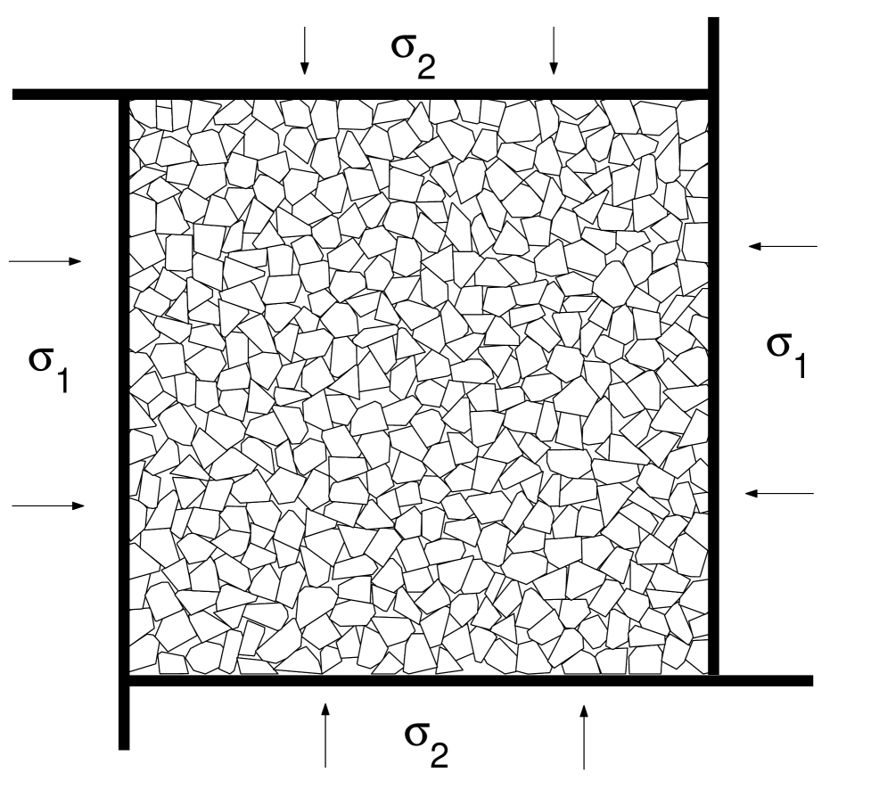
FIG. 6.: Polygonal assembly confined by a rectangular frame of walls.

A Superposition principle

We start exploring the validity of the superposition principle presented in Subsec. III C. The part (a) of Fig. 7 shows the loading path during the proportional loading under constant lateral pressure. This path is also decomposed into pieces divided into two parts: one is an incremental isotropic loading ($\Delta p=\Delta\sigma$ and $\Delta q=0$), the other is an incremental pure shear loading ($\Delta q=\Delta\sigma$ and $\Delta p=0$). The length of the steps $\Delta\sigma$ varies from to $0.4p_{0}$ to $0.001p_{0}$, where $p_{0}=640kPa$. The part (b) of Fig. 7 shows that as the steps decrease, the strain response converges to the response of the proportional loading. In order to verify this convergence, we calculate the difference between the strain response of the stair-like path $\gamma(e)$ and the proportional loading path $\gamma_{0}(e)$ as:

$$\Delta\epsilon\equiv\max_{e}{|\gamma(e)-\gamma_{0}(e)|},$$ (48)

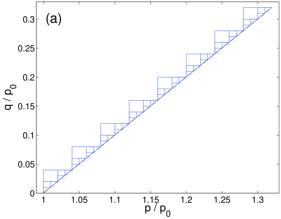
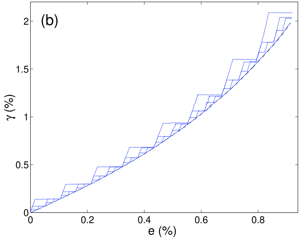
FIG. 7.: Comparison between numerical responses obtained from MD simulations of a rectilinear proportional loading (with constant lateral pressure) and stair-like paths.

for different steps sizes. This is shown in Fig. 8 for seven different polygonal assemblies. The linear interpolation of this data intersects the vertical axis at $3\times 10^{-7}$. Since this value is below the error given by the quasi-static approximation, which is $3\times 10^{-4}$, the results suggest that the responses converge to that one of the proportional load. Therefore we find that within our error bars the superposition principle is valid.

A close inspection of the incremental response will show that the validity of the superposition principle is linked to the existence of tensorial zones in the incremental stress space. Before this, a short introduction to the strain envelope responses follows.

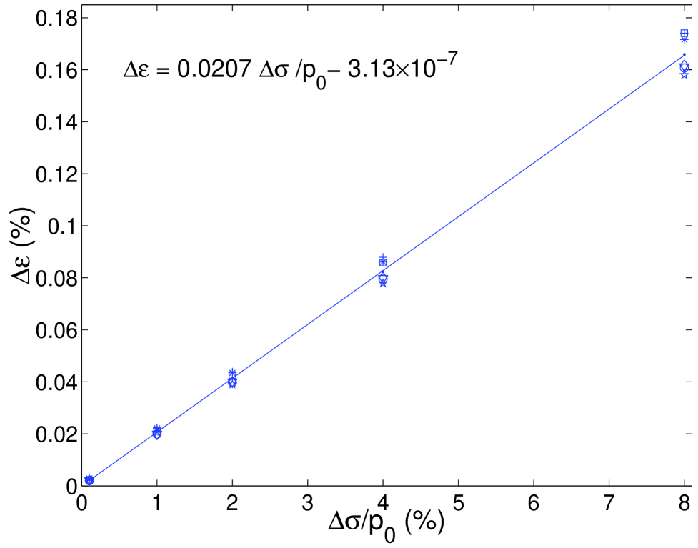
FIG. 8.: Distance between the response of the stair-like path and the proportional path.

B Incremental response

A graphical illustration of the particular features of the constitutive models can be given by employing the so-called response envelopes. They were introduced by Gudehus [17] as a useful tool to visualize the properties of a given incremental constitutive equation. The strain envelope response is defined as the image $\{d\tilde{\epsilon}={\cal G}(d\tilde{\sigma},\tilde{\sigma})\}$ in the strain space of the unit sphere in the stress space, which becomes a potato-like surface in the strain space.

In practice, the determination of the stress envelope responses is difficult because it requires one to prepare many samples with identical material properties. Numerical simulations result as an alternative to the solution of this problem. They allow one to create clones of the same sample, and to perform different loading histories in each one of them.

In the case of a plane strain tests, where there is no deformation in one of the spatial directions, the strain envelope response can be represented in a plane. According to Eq. (36), this response results in a rotated, translated ellipse in the hypoplastic theory, whereas it is given by a continuous curve consisting of two pieces of ellipses in the elasto-plastic theory, as result from Eq. (35). It is then of obvious interest to compare these predictions with the stress envelope response of the experimental tests.

Fig. 9 shows the typical strain response resulting from the different stress controlled loading in a dense packing of polygons. Each point is obtained from the strain response in a specific direction of the stress space, with the same stress amplitude of $10^{-4}p_{0}$. We take $q_{0}=0.45p_{0}$ and $p_{0}=160kPa$ In this calculation. The best fit of these results with the envelopes response of the elasto-plasticity (two pieces of ellipses). For comparison the hypoplasticity (one ellipse) is also shown in Fig. 9.

From these results we conclude that the elasto-plastic theory is more accurate in describing the incremental response of our model. One can draw to the same conclusion taking different strain values with different initial stress values [38]. These results have shown that the incremental response can be accurately described using the elasto-plastic relation of Eq. (35). The validity of this equation is supported by the existence of a well defined flow rule for each stress state.

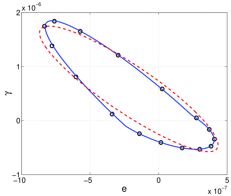
FIG. 9.: Numerical calculation of the incremental strain response. The dots are the numerical results. The solid curve represents the fit to the elasto-plastic theory. The dashed curve is the hypoplastic fit.

C Yield function

In Subsec. III B, we showed that the yield surface is an essential element in the formulation of the Drucker-Prager theory. This surface encloses a hypothetical region in the stress space where only elastic deformations are possible [18]. The determination of such a yield surface is essential to determine the dependence of the strain response on the history of the deformation.

We attempt to detect the yield surface by using a standard procedure proposed in experiments with sand [39]. Fig. 10 shows this procedure. Initially the sample is subjected to an isotropic pressure. Then the sample is loaded in the axial direction until it reaches the yield-stress state with pressure $p$ and deviatoric stress $q$. Since plastic deformation is found at this stress value, the point $(p,q)$ can be considered as a classical yield point. Then, the Drucker-Prager theory assumes the existence of a yield surface containing this point. In order to explore the yield surface, the sample is unloaded in the axial direction until it reaches the stress point with pressure $p-\Delta p$ and deviatoric stress $q-\Delta p$ inside the elastic regime. Then the yield surface is constructed by re-loading in different directions in the stress space. In each direction, the new yield point must be detected by a sharp change of the slope in the stress-strain curve, indicating plastic deformations.

Fig. 11 shows the strain response taking different load directions in the same sample. The initial stress of the sample is given by $q_{0}=0.5p_{0}$ and $p_{0}=160kPa$. If the direction of the reload path is the same as that of the original load ($45^{o}$), we observe a sharp decrease of stiffness when the load point reaches the initial yield point, which corresponds to the origin in Fig. 11. However, if one takes a direction of re-loading different from $45^{o}$, the decrease of the stiffness with the loading becomes smooth. Since there is no straightforward way to identify those points where the yielding begins, the yield function, as it was introduced by Drucker and Prager [18] in order to describe a sharp transition between the elastic and plastic regions, is not consistent with our results.

Experimental studies on dry sand seem to show that the truly elastic region is probably extremely small [4]. Moreover, a micro-mechanic investigation of the mechanical response of granular ratcheting under cyclic loading has shown that any load involves sliding contacts, and hence, plastic deformation [40]. These studies draw to the conclusion that the elastic region, used in the Drucker-Prager theory to give a dependence of the response on recent history, is not a necessary feature of granular materials.

A question that naturally rises is if the hypoplastic theory is more appropriate than the elasto-plastic models to describe soil plasticity. Since these models do not introduce any elastic regime, they seem to provide a good alternative. However, the modern versions of hypoplasticity depart from the superposition principle, which is not consistent with our results. An alternative approach to hypoplasticity can be reached from the bounding surface theory, by shrinking the elastic regime to the current stress point [41]. With this limit one can reproduce the observed continuous transition from the elastic to the elasto-plastic behavior and in the same time keep the tensorial zones. However, it has been shown that this limit leads to a constitutive relation in terms of some internal variables, which lack of physical meaning in this theory. In the author’s opinion, the necessity to provide a micro-mechanical interpretation of these internal variables will be important to capture this essential feature of mechanics of granular materials, that any loading involves plastic deformation.

FIG. 10.: Method to obtain the yield surface. Load-unload-reload tests are performed taking different directions in the reload path. In each direction, the point of the reload path where the yielding begins is marked. The yield function is constructed by connecting these points.

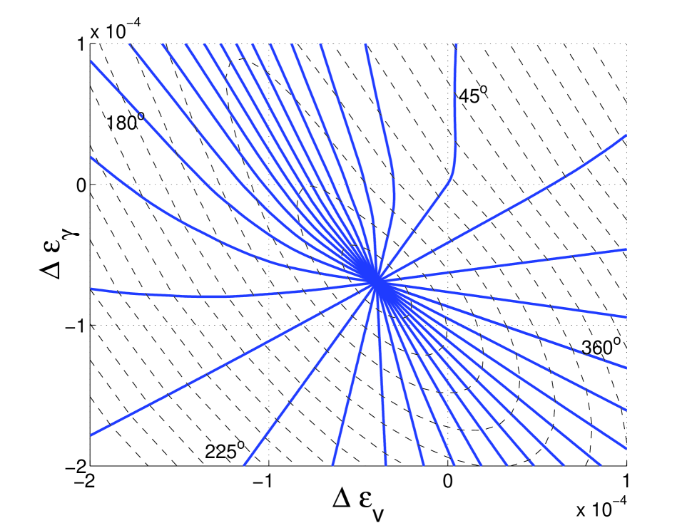
FIG. 11.: Strain responses according to Fig. 10. The solid lines show the strain response from different reload directions. The dashed contours represent the strain envelope responses for different stress increments $|\Delta\vec{\sigma}|$.

VI Instabilities

Instability has been one of the classical topics of soil mechanics. Localization from a previously homogeneous deformation to a narrow zone of intense shear is a common mode of failure of soils [20, 42, 37]. The Mohr-Coulomb criterion is typically used to understand the principal features of the localization. This criterion was improved by the Drucker condition, based on the hypothesis of the normality, which results in a plastic flow perpendicular to the yield surface [18]. This theory predicts that the instability appears when the stress of the sample reaches the plastic limit surface. This surface is given by the stress states where the plastic deformation becomes infinite. In previous work, it is shown that the normality postulate is not fulfilled in the incremental response of this model, because the flow and yield directions of Eq. (34) are different [38]. Thus, it is interesting to see if the Drucker stability criterion is still valid.

According to the flow rule of Eq. (34), the plastic limit surface can be found by looking for the stress values where the plastic modulus vanishes. The dependence of this modulus on the stress fits to the following power law relation [38]:

$$h=h_{0}\left[1-\frac{q}{q_{0}}(\frac{p_{0}}{p})^{\vartheta}\right]^{\eta}.$$ (49)

This is given in terms of the four parameters: The plastic modulus $h_{0}=14.5\pm 0.05$ at $q=0$, the constant $q_{0}=0.85\pm 0.05$, and the exponents $\eta=2.7\pm 0.04$ and $\vartheta=0.99\pm 0.02$. Then, the plastic limit surface is given by the stress states with zero plastic modulus:

$$\frac{q_{p}}{q_{0}}=\left(\frac{p}{p_{0}}\right)^{\vartheta}.$$ (50)

On the other hand, the failure surface can be defined by the limit of the stress values where the material becomes unstable. It has been shown that this is given by the following relation [38]

$$\frac{q}{q_{c}}=\left(\frac{p}{p_{0}}\right)^{\beta}.$$ (51)

Here $p_{0}=1.0MPa$ is the reference pressure, and $q_{c}=0.78\pm 0.03MPa$. The power law dependence on the pressure, with exponent $\beta=0.92\pm 0.02$ implies a small deviation from the Mohr-Coulomb theory where the relation is strictly linear.

By comparing Eq. (51) to Eq. (50) one observes that during loading the instabilities appear before reaching the plastic limit surface. Theoretical studies have also shown that in the case of non-associated materials, (i.e. where flow direction does not agree with the yield direction) the instabilities can appear strictly inside of the plastic limit surface [16]. In this context, the question of instability must be reconsidered beyond the Drucker condition.

The stability for non-associated elasto-plastic materials has been investigated by Hill, who established the following sufficient stability criterion [43].

$$\forall d\tilde{\epsilon},~{}~{}~{}d\tilde{\sigma}\cdot d\tilde{\epsilon}>0.$$ (52)

The analysis of this criterion of stability will be presented here based on the constitutive relation given by Eq. (35). The stability condition of this constitutive relation can be evaluated by introducing the normalized second order work [16]:

$$d^{2}W\equiv\frac{d\tilde{\sigma}\cdot d\tilde{\epsilon}}{|d\tilde{\sigma}|^{2}}$$ (53)

Then, the Hill condition of stability can be obtained by replacing Eq. (35) in this expression. This results in

$$d^{2}W=\hat{\sigma}D^{-1}\hat{\sigma}+\frac{\langle\cos(\theta+\phi)\rangle}{h}\cos(\theta+\psi)>0,$$ (54)

where $\hat{\sigma}$ was defined in Eq. (24). In the case where the Drucker normality postulate $\psi=\phi$ is valid, Eq. (54) is strictly positive and, therefore, this stability condition would be valid for all the stress states inside the plastic limit surface . On the contrary, for a non-associated flow rule as in our model, the second order work is not strictly positive for all the load directions, and it can take zero values inside the plastic limit surface (i.e. during the hardening regime where $h>0$).

To analyze this instability, we adopt a circular representation of $d^{2}W$ shown in Fig. 12. The dashed circles in these figures represent those regions where $d^{2}W<0$. For stress ratios below $q/p=0.7$ we found that the second order work is strictly positive. Thus, according to the Hill stability condition, this region corresponds to stable states. For the stress ratio $q/p=0.8$, the second order work becomes negative between $27^{o}<\theta<36^{o}$ and $206^{o}<\theta<225^{o}$. This leads to a domain of the stress space strictly inside the plastic limit surface where the Hill condition of stability is not fulfilled, and therefore the material is potentially unstable.

Numerical simulations of biaxial tests show that strain localization is the most typical mode of failure [7, 44]. The fact that it appears before the sample reaches the plastic limit surface suggests that the appearance of this instability is not completely determined by the current macroscopic stress of the material, as it is predicted by the Drucker-Prager theory. More recent analytic [45] and experimental [37, 36] works have focused on the role of the micro-structure on the localized instabilities. Frictional slips at the particles have been used to define additional degrees of freedom [45]. The introduction of the particle diameter in the constitutive relations results in a correct prediction of the shear band thickness. The new degrees of freedom of these constitutive models are still not clearly connected to the micro-mechanical variables of the grains, but with the development of numerical simulations this aspect can be better understood.

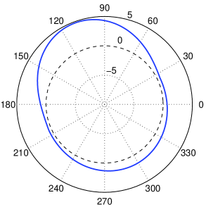
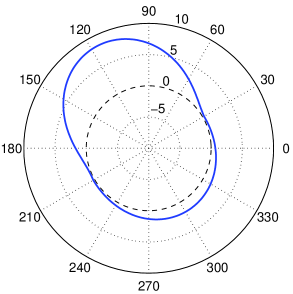
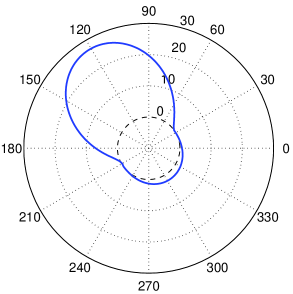
FIG. 12.: The solid lines show the second order work as a function of the direction of load for three different stress ratios $q/p=0.6$ (left), $0.7$ (center), and $0.65$ (right) with pressure $p=160KPa$. The dashed circles enclose the region where $d^{2}W<0$.

VII Concluding remarks

In this paper we have obtained explicit expressions for the averaged stress and strain tensors over a RVE, in terms of the micro-mechanical variables, contact forces and the individual displacements and rotations of the grains.

A short review on the incremental non-linear models has been presented. We emphasize the existence of the elastic regime, and the two tensorial zones as predicts the theory of elasto-plasticity. We consider also the superposition principle of soil mechanics, which is not satisfied in the incremental non-linear models. These assumptions have been studied using molecular dynamics simulations on a polygonal packing. The results are summarized as follows:

• The elasto-plastic theory, with two tensorial zones, provided a more accurate description of the incremental response than the hypoplastic theory.

• In contradiction to the incremental non-linear models, the simulation results show that the superposition principle is accurately satisfied.

• The experimental method proposed by Tatsouka has been implemented to identify the yield surface. The resulting strain response shows that the transition from elasticity to elasto-plasticity is not as sharp as the Drucker-Prager theory predicts, but a smooth transition occurs. The fact that there is no purely elastic regime leads to the open question of how to determine the dependence of the response of soils on the history of the deformation.

• The calculation of the plastic limit condition and the failure surface shows that the failure appears during the hardening regime $h>0$. This result is analyzed using the Hill condition of stability, which states that for non-associated materials the instabilities can appear before the plastic limit surface.

These conclusions appear to contradict both the Drucker-Prager theory and the hypoplastic models. In future work, it would be important to revisit the question of the incremental non-linearity of soils from micro-mechanical considerations.

REFERENCES

- [1] L.D. Landau and E. M. Lifshitz. Theory of Elasticity. Pergamon Press, Moscou, 1986. Volume 7 of Course of Theoretical Physics.
- [2] P. A. Vermeer. Non-associated plasticity for soils, concrete and rock. In Physics of dry granular media - NATO ASI Series E350, page 163, Dordrecht, 1998. Kluwer Academic Publishers.
- [3] K. H. Roscoe and J. B. Burland. On the generalized stress-strain behavior of ’wet’ clay. In Engineering Plasticity, pages 535–609, Cambridge, 1968. Cambridge University Press.
- [4] G. Gudehus, F. Darve, and I. Vardoulakis. Constitutive Relations of soils. Balkema, Rotterdam, 1984.
- [5] P. A. Cundall and O. D. L. Strack. A discrete numerical model for granular assemblages. Géotechnique, 29:47–65, 1979.
- [6] K. Bagi. Stress and strain in granular assemblies. Mech. of Materials, 22:165–177, 1996.
- [7] P. A. Cundall, A. Drescher, and O. D. L. Strack. Numerical experiments on granular assemblies; measurements and observations. In IUTAM Conference on Deformation and Failure of Granular Materials, pages 355–370, Delft, 1982. Balkema,Rotterdam.
- [8] C. Goldenberg and I. Goldhirsch. Force chains, microelasticity, and macroelasticity. Phys. Rev. Lett., 89(8):084302, 2002.
- [9] K. Bagi. Microstructural stress tensor of granular assemblies with volume forces. J. Appl. Mech., 66:934–936, 1999.
- [10] M. Lätzel. From discontinuous models towards a continuum description of granular media. PhD thesis, Universität Stuttgart, 2002.
- [11] J. P. Bardet. Numerical simulations of the incremental responses of idealized granular materials. Int. J. Plasticity, 10:879–908, 1994.
- [12] Y. Kishino. On the incremental nonlinearity observed in a numerical model for granular media. Italian Geotechnical Journal, 3:3–12, 203.
- [13] F. Calvetti, G. Viggiani, and C. Tamagnini. Micromechanical inspection of constitutive modelling. In Constitutive modelling and analysis of boundary value problems in Geotechnical Engineering, pages 187–216., Benevento, 2003. Hevelius Edizioni.
- [14] M. Oda and K. Iwashita. Study on couple stress and shear band development in granular media based on numerical simulation analyses. Int. J. of Enginering Science, 38:1713–1740, 2000.
- [15] R. J. Bathurst and L. Rothenburg. Micromechanical aspects of isotropic granular assemblies with linear contact interactions. J. Appl. Mech., 55:17–23, 1988.
- [16] F. Darve and F. Laouafa. Instabilities in granular materials and application to landslides. Mechanics of Cohesive-Frictional Materials, 5:627–652, 2000.
- [17] G. Gudehus. A comparison of some constitutive laws for soils under radially symmetric loading and unloading. Can. Geotech. J., 20:502–516, 1979.
- [18] D.C. Drucker and W. Prager. Soil mechanics and plastic analysis of limit design. Q. Appl. Math., 10(2):157–165, 1952.
- [19] R. Nova and D. Wood. A constitutive model for sand in triaxial compression. Int. J. Num. Anal. Meth. Geomech., 3:277–299, 1979.
- [20] K. H. Roscoe. The influence of the strains in soil mechanics. Geotechnique, 20(2):129–170, 1970.
- [21] H. B. Poorooshasb, I. Holubec, and A. N. Sherbourne. Yielding and flow of sand in triaxial compression. Can. Geotech. J., 4(4):277–398, 1967.
- [22] E. M. Wood. Soil Mechanics-transient and cyclic loads. Chichester, 1982.
- [23] Y. F. Dafalias and E. P. Popov. A model of non-linearly hardening material for complex loading. Acta Mechanica, 21:173–192, 1975.
- [24] D. Kolymbas. An outline of hypoplasticity. Arch. Appl. Mech., 61:143–151, 1991.
- [25] F. Darve, E. Flavigny, and M. Meghachou. Yield surfaces and principle of superposition: revisit through incrementally non-linear constitutive relations. International Journal of Plasticity, 11(8):927, 1995.
- [26] R. Chambon, J. Desrues, W. Hammad, and R. Charlier. CLoE, a new rate type constitutive model for geomaterials. Theoretical basis and implementation. Int. J. Anal. Meth. Geomech., 18:253–278, 1994.
- [27] W. Wu, E. Bauer, and D. Kolymbas. Hypoplastic constitutive model with critical state for granular materials. Mech. Matter., 23:45–69, 1996.
- [28] I. Herle and G. Gudehus. Determination of parameters of a hypoplastic constitutive model from properties of grain assemblies. Mechanics of Cohesive-Frictional Materials, 4:461–486, 1999.
- [29] D. Kolymbas. Modern Approaches to Plasticity. Elsevier, 1993.
- [30] F. Kun and H. J. Herrmann. Transition from damage to fragmentation in collision of solids. Phys. Rev. E, 59(3):2623–2632, 1999.
- [31] C. Moukarzel and H. J. Herrmann. A vectorizable random lattice. Journal of Statistical Physics, 68(5/6):911–923, 1992.
- [32] A. Okabe, B. Boots, and K. Sugihara. Spatial Tessellations. Concepts and Applications of Voronoi Diagrams. John Wiley & Sons, Chichester, 1992. Wiley Series in probability and Mathematical Statistics.
- [33] H. J. Tillemans and H. J. Herrmann. Simulating deformations of granular solids under shear. Physica A, 217:261–288, 1995.
- [34] M. P. Allen and D. J. Tildesley. Computer Simulation of Liquids. Oxford University Press, Oxford, 1987.
- [35] E. Buckingham. On physically similar systems: Illustrations of the use of dimensional equations. Phys. Rev., 4:345–376, 1914.
- [36] T. Marcher and P. A. Vermeer. Macromodelling of softening in non-cohesive soils. In Continuous and Discontinuous Modelling of Cohesive Frictional Materials, pages 89–110, Berlin, 2001. Springer.
- [37] J. Desrues. Localisation de la deformation plastique dans les materieux granulaires. PhD thesis, University of Grenoble, 1984.
- [38] F. Alonso-Marroquin and H.J. Herrmann. Calculation of the incremental stress-strain relation of a polygonal packing. Phys. Rev. E, 66:021301, 2002. cond-mat/0203476.
- [39] Tatsouka F and K. Ishihara. Yielding of sand in triaxial compression. Soils and Fundations, 14(2):63–76, 1974.
- [40] F. Alonso-Marroquin and H.J. Herrmann. Ratcheting of granular materials. Phys. Rev. Lett., 92(5):054301, 2004.
- [41] Y. F. Dafalias. Bounding surface plasticity. I: Mathematical foundation and hypoplassticity. J. of Engng. Mech, 112(9):966–987, 1986.
- [42] P. A. Vermeer. A five-constant model unifying well-established concepts. In Constitutive Relations of soils, pages 175–197, Rotterdam, 1984. Balkema.
- [43] R. Hill. A general theory of uniqueness and stability in elastic-plas tic solids. Journal of Geotechnical Engineering, 6:239–249, 1958.
- [44] J. A. Astrøm, H.J.Herrmann, and J. Timonen. Granular packings and fault zones. Phys. Rev. Lett., 84:4638–4641, 2000.
- [45] H.-B. Mühlhaus and I. Vardoulakis. The thickness of shear bands in granular materials. Géotechnique, (37):271–283, 1987.