The anisotropy of granular materials

Abstract

The effect of the anisotropy on the elastoplastic response of two dimensional packed samples of polygons is investigated here, using molecular dynamics simulation. We show a correlation between fabric coefficients, characterizing the anisotropy of the granular skeleton, and the anisotropy of the elastic response. We also study the anisotropy induced by shearing on the subnetwork of the sliding contacts. This anisotropy provides an explanation to some features of the plastic deformation of granular media.

I Introduction

The mechanical behavior of granular materials has been largely investigated using constitutive models. These are empirical relations which are based on, for example, laboratory tests of soil specimens. On the other hand, the investigation of the soils at the grain scale, using discrete element modeling, has become possible in recent years. These models have provided a valuable understanding of many micro-mechanical aspects of soil deformation. In particular, numerical simulations of packings of disks evidence that the stress applied on the boundary of the assembly is transmitted through a heterogeneous network of interparticle contacts [1]. The geometric change of this network during deformation shows a structural anisotropy induced by shearing [2, 3, 4]. Numerical simulations have also shown a relevant number of contacts reaching the sliding condition, even when the sample is isotropically compressed [5, 1]. However, little work has been done in order to connect the sliding at the contacts to the plastic deformation of granular materials. The aim of this paper is to combine the continuous and the discrete approaches in the investigation of the anisotropic response of granular materials, taking into account the anisotropy induced in both sliding and non-sliding contacts.

We will numerically study the elasto-plastic response of a two-dimensional granular model material. The interparticle forces include elasticity, viscous damping and friction with the possibility of slippage. The system is driven by applying stress controlled tests at the boundary particles. The results show that the traditional fabric tensor is not sufficient to describe the complex elasto-plastic response of granular materials. Additional parameters taking into account the anisotropy of the subnetwork of the sliding contacts are necessary to include in the description of the overall plastic deformations.

This paper is organized as follows: The details of the particle model are presented in Sec. II. The contact forces are implemented by a Coulomb friction criterion, and the stress is controlled by the application of suitable forces at the boundary particles. The calculation of the constitutive relations is presented in Sec. III. Here we discuss the results in the framework of the Drucker-Prager theory of elasto-plasticity. In Sec. IV we study the effect of the anisotropy of the contact network in the incremental elastic response of the assembly. In Sec. V some internal variables are introduced in the constitutive relations. These variables take into account the effect of the anisotropy induced in the subnetwork of the sliding contacts on the plastic deformation of the assembly.

II Model

We present here an extension of those two-dimensional discrete element methods which have been used to model granular materials via polygonal particles [6, 7]. The details of the particle generation, the contact forces, the boundary conditions and the molecular dynamics simulations are presented in this section.

A Generation of polygons

The polygons representing the particles in this model are generated by using the method of Voronoi tessellation [7]. This methods is schematically shown in Fig. 1: First, a regular square lattice of side $\ell$ is created. Then, we choose a random point in each cell of the rectangular grid. Then, each polygon is constructed assigning to each point that part of the plane that is nearer to it than to any other point. The details of the construction of the Voronoi cells can be found in the literature [8, 9].

Using the Euler theorem, it has been shown analytically that the mean number of edges of this Voronoi construction must be six [9]. The number of edges of the polygons is distributed between $4$ and $8$ for $98.7\%$ of the polygons. We also found that the orientational distribution of edges is isotropic, and the distribution of areas of polygons is symmetric around its mean value $\ell^{2}$. The probabilistic distribution of areas follows approximately a Gaussian distribution with variance of $0.36\ell^{2}$.

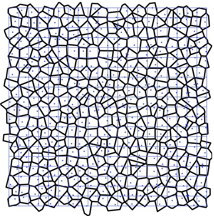
FIG. 1.: Voronoi construction used to generate the convex polygons. The dots indicate the point used in the tessellation. Periodic boundary conditions were used.

B Contact forces

In order to give a three-dimensional picture of this model, one can consider the polygons as a collection of prismatic bodies with randomly-shaped polygonal basis. We assume that all the bodies have the same thickness $L$. The force between two polygons is written as $\vec{F}=L\vec{f}$ and the mass of the polygons is $M=Lm$.

In reality, when two elastic bodies come into contact, they have a slight deformation in the contact region. In the calculation of the contact force we suppose that the polygons are rigid, but we allow them to overlap. Then, we calculate the force from this virtual overlap.

The first step for the calculation of the contact force is the definition of the line representing the flattened contact surface between the two bodies in contact. This is defined from the contact points resulting from the intersection of the edges of the overlapping polygons. In most cases, we have two contact points, as shown in the left of Fig. 2. In such a case, the contact line is defined by the vector $\vec{C}=\overrightarrow{C_{1}C_{2}}$ connecting these two intersection points. In some pathological cases, the intersection of the polygons leads to four or six contact points. In these cases, we define the contact line by the vector $\vec{C}=\overrightarrow{C_{1}C_{2}}+\overrightarrow{C_{3}C_{4}}$ or $\vec{C}=\overrightarrow{C_{1}C_{2}}+\overrightarrow{C_{3}C_{4}}+\overrightarrow{C_{5}C_{6}}$, respectively. This choice guarantees a continuous change of the contact line, and therefore of the contact forces, during the evolution of the contact.

FIG. 2.: Contact points $C_{i}$ before (left) and after the formation of a pathological contact (right). The vector denotes the contact line. $t$ represents the time step.

The contact force is separated as $\vec{f}^{c}=\vec{f}^{e}+\vec{f}^{v}$, where $\vec{f}^{e}$ and $\vec{f}^{v}$ are the elastic and viscous contribution. The elastic part of the contact force is decomposed as $\vec{f^{e}}=f^{e}_{n}\hat{n}^{c}+f^{e}_{t}\hat{t}^{c}$. The calculation of these components is explained below. The unit tangential vector is defined as $\hat{t}^{c}=\vec{C}/|\vec{C}|$, and the normal unit vector $\hat{n}^{c}$ is taken perpendicular to $\vec{C}$. The point of application of the contact force is taken as the center of mass of the overlapping polygons.

As opposed to the Hertz theory for round contacts, there is no exact way to calculate the normal force between interacting polygons. An alternative method has been proposed in order to model this force[6]. In this method, normal elastic force is calculated as $f^{e}_{n}=-k_{n}A/L_{c}$ where $k_{n}$ is the normal stiffness, $A$ is the overlapping area and $L_{c}$ is a characteristic length of the polygon pair. Our choice is $L_{c}=|\vec{C}|$. This normalization is necessary to reflect the fact that the normal elastic force must be proportional to an overlapping length as it was shown in bidimensional Hertzian contacts [10].

In order to model the quasi-static friction force, we calculate the elastic tangential force using an extension of the method proposed by Cundall-Strack [11]. An elastic force $f^{e}_{t}=-k_{t}\Delta x_{t}$ proportional to the elastic displacement is included at each contact. $k_{t}$ is the tangential stiffness. The elastic displacement $\Delta x_{t}$ is calculated as the time integral of the tangential velocity of the contact during the time where the elastic condition $|f^{e}_{t}|<\mu f^{e}_{n}$ is satisfied. The sliding condition is imposed, keeping this force constant when $|f^{e}_{t}|=\mu f^{e}_{n}$. The straightforward calculation of this elastic displacement is given by the time integral starting at the beginning of the contact:

$$\Delta x^{e}_{t}=\int_{0}^{t}v^{c}_{t}(t^{\prime})\Theta(\mu f^{e}_{n}-|f^{e}_{t}|)dt^{\prime},$$ (1)

where $\Theta$ is the Heaviside step function and $\vec{v}^{c}_{t}$ denotes the tangential component of the relative velocity $\vec{v}^{c}$ at the contact.

$$\vec{v}^{c}=\vec{v}_{i}-\vec{v}_{j}-\vec{\omega}_{i}\times\vec{\ell}_{i}+\vec{\omega}_{j}\times\vec{\ell}_{j}.$$ (2)

Here $\vec{v}_{i}$ is the linear velocity and $\vec{\omega}_{i}$ is the angular velocity of the particles in contact. The branch vector $\vec{\ell}_{i}$ connects the center of mass of particle $i$ with the point of application of the contact force. Eq. (1) allows to keep $\Delta x_{t}$ at a length such that $|f^{e}_{t}|$ agrees with $\mu f^{e}_{n}$ during the sliding condition.

Damping forces are included in order to allow for rapid relaxation during the preparation of the sample, and to reduce the acoustic waves produced during the loading. These forces are calculated as

$$\vec{f}^{c}_{v}=-m(\gamma_{n}v^{c}_{n}\hat{n}^{c}+\gamma_{t}v^{c}_{t}\hat{t}^{c}),$$ (3)

with $m=(1/m_{i}+1/m_{j})^{-1}$, the effective mass of the polygons in contact. $\hat{n}^{c}$ and $\hat{t}^{c}$ are the normal and tangential unit vectors defined before, and $\gamma_{n}$ and $\gamma_{t}$ are the coefficients of viscosity. These forces introduce time dependent effects during the cyclic loading. However, we will show that these effects can be arbitrarily reduced by increasing the loading time, as it corresponds to the quasi-static approximation.

C Molecular dynamics simulation

The evolution of the position $\vec{x}_{i}$ and the orientation $\varphi_{i}$ of the polygon $i$ is governed by the equations of motion:

$$m_{i}\ddot{\vec{x}}_{i} = \sum_{c}\vec{f^{c}_{i}}+\sum_{b}\vec{f}^{b}_{i},$$ (4)

$$I_{i}\ddot{\varphi}_{i} = \sum_{c}\vec{\ell}^{c}_{i}\times\vec{f^{c}_{i}}+\sum_{b}\vec{\ell}^{b}_{i}\times\vec{f}^{b}_{i}.$$ (5)

Here $m_{i}$ and $I_{i}$ are the mass and moment of inertia of the polygon $i$. The first summation goes over all particles in contact with this polygon. According to the previous section, these forces $\vec{f^{c}}$ are given by

$$\vec{f^{c}} = -(k_{n}A/L_{c}+\gamma mv^{c}_{n})\vec{n}^{c}-(\Delta x^{c}_{t}+\gamma_{n}mv^{c}_{t})\vec{t}^{c},$$ (6)

The second summation on the left hand side of Eq. (5) goes over all the edges of the polygons in contact with the external contour of the assembly. We apply a force

$$\vec{f}^{b}=-\sigma_{1}\Delta x^{b}_{2}\hat{x_{1}}+\sigma_{3}\Delta x^{b}_{1}\hat{x}_{2}-m_{i}\gamma_{b}\vec{v_{i}}.$$ (8)

on each selected segment $\vec{T}^{b}=\Delta x^{b}_{1}\hat{x}_{1}+\Delta x^{b}_{2}\hat{x}_{2}$ of the external contour of the assembly. Here $\hat{x}_{1}$ and $\hat{x}_{2}$ are the unit vectors of the Cartesian coordinate system. $\sigma_{1}$ and $\sigma_{3}$ are the components of the stress we want to apply on the sample, as we see in Subsec. III. $m_{i}$ and $\vec{v}_{i}$ are the mass and the velocity of the particle $i$ belonging to the boundary. $\vec{\ell}^{b}$ is the vector connecting the center of mass of the boundary particle $i$ to the center of the boundary segment $\vec{T}^{b}$.

We use a fifth-order Gear predictor-corrector method for solving the equation of motion [12]. This algorithm consists of three steps. The first step predicts position and velocity of the particles by means of a Taylor expansion. The second step calculates the forces as a function of the predicted positions and velocities. The third step corrects the positions and velocities in order to optimize the stability of the algorithm. This method is much more efficient than the simple Euler approach or the Runge-Kutta method, especially for problems where very high accuracy is a requirement.

The parameters of the molecular dynamics simulations were adjusted according to the following criteria: 1) guarantee the stability of the numerical solution, 2) optimize the time of the calculation, and 3) provide a reasonable agreement with the experimental data.

There are many parameters in the molecular dynamics algorithm. Before choosing them, it is convenient to make a dimensional analysis. In this way, we can keep the scale invariance of the model and reduce the parameters to a minimum of dimensionless constants. First, we introduce the following characteristic times of the simulations: the loading time $t_{0}$, the relaxation times $t_{n}=1/\gamma_{n}$, $t_{t}=1/\gamma_{t}$, $t_{b}=1/\gamma_{b}$ and the characteristic period of oscillation $t_{s}=\sqrt{k_{n}/\rho\ell^{2}}$ of the normal contact.

Using the Buckingham Pi theorem [13], one can show that the strain response, or any other dimensionless variable measuring the response of the assembly during loading, depends only on the following dimensionless parameters: $\alpha_{1}=t_{n}/t_{s}$, $\alpha_{2}=t_{t}/t_{s}$, $\alpha_{3}=t_{b}/t_{s}$, $\alpha_{4}=t_{0}/t_{s}$, the ratio $\zeta=k_{t}/k_{n}$ between the stiffnesses, the friction coefficient $\mu$ and the ratio $\sigma_{i}/k_{n}$ between the stresses and the normal stiffness.

The variables $\alpha_{i}$ will be called control parameters. They are chosen in order to satisfy the quasi-static approximation, i.e. the response of the system does not depend on the loading time, but a change of these parameters within this limit does not affect the strain response. $\alpha_{2}=0.1$ and $\alpha_{2}=0.5$ were taken large enough to have a high dissipation, but not too large to keep the numerical stability of the method. $\alpha_{3}=0.001$ is chosen by optimizing the time of consolidation of the sample during the application of the confining pressure. The ratio $\alpha_{4}=t_{0}/t_{s}=10000$ was chosen large enough in order to avoid rate-dependence in the strain response, corresponding to the quasi-static approximation. Technically, this is performed by looking for the value of $\alpha_{4}$ such that a reduction of it by half makes a change of the stress-strain relation less than $5\%$.

The parameters $\zeta$ and $\mu$ can be considered as material parameters. They determine the constitutive response of the system, so they must be adjusted with the experimental data. In this study, we have adjusted them by comparing the simulation of biaxial tests of dense polygonal packings with the corresponding tests with dense Hostun sand [14]. First, the initial Young modulus of the material is linearly related to the value of normal stiffness of the contact. Thus, $k_{n}=160MPa$ is chosen by fitting the initial slope of the stress-strain relation in the biaxial test. Then, the Poisson ratio depends on the ratio $\zeta=k_{t}/k_{n}$. Our choice $k_{t}=52.8MPa$ gives an initial Poisson ratio of $0.07$. This is obtained from the initial slope of the curve of volumetric strain versus axial strain. The angles of friction and the dilatancy are increasing functions of the friction coefficient $\mu$. Taking $\mu=0.25$ yields angles of friction of $30-40$ degrees and dilatancy angles of $20-30$ degrees. The experimental data yields angles of friction between $40-45$ degrees and dilatancy angles between $7-14$ degrees. A better adjustment would be made by including different void ratios in the simulations, but this is out of the scope of this work.

III stress-strain relation

The characterization of the macroscopic state of a granular material in static equilibrium is usually given by the Cauchy stress tensor. The average of this tensor over the assembly leads to [15]

$$\sigma_{ij}=\frac{1}{A}\sum_{b}x^{b}_{i}f^{b}_{j}$$ (9)

The sum goes over all the forces acting over the boundary of the assembly. $\vec{x}^{b}$ is the point of application of the boundary force $\vec{f}^{b}$. This force is defined in Eq. (8). $A$ is the area enclosed by the boundary. The sum goes over all the boundary forces of the sample. Inserting Eq. (8) in Eq. (9) and taking the equilibrium condition $\vec{v}_{i}=0$ leads to

$$\sigma=\frac{1}{A}\left[\begin{array}[]{cc}-\sigma_{1}\sum_{b}{x_{b}\Delta y_{b}}&\sigma_{3}\sum_{b}{x_{b}\Delta x_{b}}\\ -\sigma_{1}\sum_{b}{y_{b}\Delta y_{b}}&\sigma_{3}\sum_{b}{y_{b}\Delta x_{b}}\end{array}\right].$$ (10)

Those sums can be converted into integrals over closed loops and the calculation of such integrals leads to

$$\sigma=\left[\begin{array}[]{cc}\sigma_{1}&0\\ 0&\sigma_{3}\end{array}\right].$$ (11)

Thus, the stress controlled test is restricted to stress states without off-diagonal components. So we can simplify the notation introducing the pressure $p$ and the deviatoric stress $q$ in the components of the stress vector

$$\tilde{\sigma}=\left[\begin{array}[]{c}p\\ q\end{array}\right]=\frac{1}{2}\left[\begin{array}[]{c}\sigma_{1}+\sigma_{3}\\ \sigma_{1}-\sigma_{3}\end{array}\right].$$ (12)

In the same way, the incremental strain tensor can be calculated from the average of the displacement gradient over the area of the RVE. It has been shown [16] that it can be transformed in a sum over the boundary of the sample

$$d\epsilon_{ij}=\frac{1}{2A}\sum_{b}{(\Delta u^{b}_{i}N^{b}_{j}+\Delta u^{b}_{j}N^{b}_{i})}$$ (13)

Here $\Delta\vec{u}^{b}$ is the displacement of the boundary segment, that is calculated from the linear displacement $\Delta\vec{x}$ and the angular rotation $\Delta\vec{\phi}$ of the polygons belonging to it, according to

$$\Delta\vec{u}^{b}=\Delta\vec{x}+\Delta\vec{\phi}\times\vec{\ell}.$$ (14)

From the eigenvalues $d\epsilon_{1}$ $d\epsilon_{3}$ of $d\epsilon_{ij}$ we define the volumetric and deviatoric components of the strain as the components of the incremental strain vector:

$$d\tilde{\epsilon}=\left[\begin{array}[]{c}de\\ d\gamma\end{array}\right]=-\left[\begin{array}[]{c}d\epsilon_{1}+d\epsilon_{3}\\ d\epsilon_{1}-d\epsilon_{3}\end{array}\right].$$ (15)

By convention $de>0$ corresponds to a compression of the sample. We are going to assume a rate-independent constitutive relation between the incremental stress and incremental strain tensor. In this case the incremental relation can generally be written as [17]:

$$d\tilde{\epsilon}=M(\hat{\theta},\tilde{\sigma})d\tilde{\sigma},$$ (16)

where $\hat{\theta}$ is the unitary vector defining a specific direction in the stress space:

$$\hat{\theta}=\frac{d\tilde{\sigma}}{|d\tilde{\sigma}|}\equiv\left[\begin{array}[]{c}\cos\theta\\ \sin\theta\end{array}\right],~{}~{}|d\tilde{\sigma}|=\sqrt{dp^{2}+dq^{2}}.$$ (17)

The constitutive relation results from the calculation of $d\tilde{\epsilon}(\theta)$, where each value of $\theta$ is related to a particular mode of loading. Some special modes are listed in Table I.

In order to compare the resulting incremental response to the elasto-plastic theory, it is necessary to assume that the incremental strain can be separated into an elastic (recoverable) and a plastic (unrecoverable) component:

$$d\tilde{\epsilon}=d\tilde{\epsilon}^{e}+d\tilde{\epsilon}^{p},$$ (18)

$$d\tilde{\epsilon}^{e}=D^{-1}(\tilde{\sigma})d\tilde{\sigma},$$ (19)

$$d\tilde{\epsilon}^{p}=J(\theta,\tilde{\sigma})d\tilde{\sigma}.$$ (20)

$0^{o}$	isotropic compression	$dp>0$	$dq=0$
$45^{o}$	axial loading	$d\sigma_{1}>0$	$d\sigma_{3}=0$
$90^{o}$	pure shear	$dp=0$	$dq>0$
$135^{o}$	lateral loading	$d\sigma_{1}=0$	$d\sigma_{3}>0$
$180^{o}$	isotropic expansion	$dp<0$	$dq=0$
$225^{o}$	axial stretching	$d\sigma_{1}<0$	$d\sigma_{3}=0$
$270^{o}$	pure shear	$dp=0$	$dq<0$
$315^{o}$	lateral stretching	$d\sigma_{1}=0$	$d\sigma_{3}<0$

TABLE I.: Principal modes of loading according to the orientation of $\hat{\theta}$

Here, $D^{-1}$ is the inverse of the stiffness tensor $D$, and $J=M-D^{-1}$ the flow rule of plasticity [18]. They can be obtained from the calculation of $d\tilde{\epsilon}^{e}(\theta)$ and $d\tilde{\epsilon}^{p}(\theta)$ as we will see below.

The method presented here to calculate the strain response has been used on sand experiments [19]. It was introduced by Bardet [20] in the calculation of the incremental response using discrete element methods. This method will be used to determine the elastic $d\tilde{\epsilon}^{e}$ and plastic $d\tilde{\epsilon}^{p}$ components of the strain as function of the stress state $\tilde{\sigma}$ and the stress direction $\hat{\theta}$.

First, it is isotropically compressed until it reaches the stress value $\sigma_{1}=\sigma_{3}=p-q$. Next, it is subjected to axial loading in order to increase the axial stress $\sigma_{1}$ to $p+q$. When the stress state with pressure $p$ and deviatoric stress $q$ is reached, the sample is allowed to relax. Loading the sample from $\tilde{\sigma}$ to $\tilde{\sigma}+d\tilde{\sigma}$ the strain increment $d\tilde{\epsilon}$ is obtained. Then the sample is unloaded to $\tilde{\sigma}$ and one finds a remaining strain $d\tilde{\epsilon}^{p}$, that corresponds to the plastic component of the incremental strain. For small stress increments the unloaded stress-strain path is almost elastic. Thus, the difference $d\tilde{\epsilon}^{e}=d\tilde{\epsilon}-d\tilde{\epsilon}^{p}$ can be taken as the elastic component of the strain. This procedure is implemented on different ”clones” of the same sample, choosing different stress directions and the same stress amplitude in each one of them.

This method is based on the assumption that the strain response after a reversal loading is completely elastic. However, numerical simulations have shown that this assumption is not strictly true, because sliding contacts are always observed during the unload path [21, 5]. In order to overcome this difficulty, Calvetti et al. [21] calculate the elastic part by removing the frictional condition setting $\mu=\infty$, and measuring the purely elastic response $d\tilde{\epsilon}^{ns}$ of the assembly. Then the plastic component of the strain can be calculated as $d\tilde{\epsilon}^{p}=d\tilde{\epsilon}-d\tilde{\epsilon}^{ns}$.

In our simulations, we have observed that the plastic deformation during the reversal stress path is less than $1\%$ of the corresponding value of the elastic response. Within this margin of error, the method proposed by Bardet can be taken as a reasonable approximation to describe the elasto-plastic response.

Fig. 3 shows the load-unload stress paths and the corresponding strain response when an initial stress state with $\sigma_{1}=200kPa$ and $\sigma_{3}=120kPa$ is chosen. The end of the load paths in the stress space maps into a strain envelope response $d\tilde{\epsilon}(\theta)$ in the strain space. Likewise, the end of the unload paths maps into a plastic envelope response $d\tilde{\epsilon}^{p}(\theta)$. The yield direction $\phi$ can be found from this response, as the direction in the stress space where the plastic response is maximal. In this example, this is around $\theta=87.2^{o}$. The flow direction $\psi$ is given by the direction of the maximal plastic response in the strain space, which is around $76.7^{o}$. The fact that these directions do not agree reflects a non-associated flow rule, as it is observed in experiments on realistic soils [19].

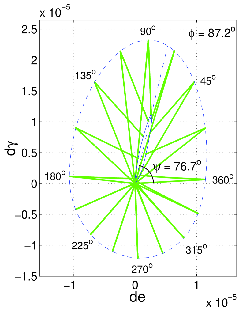
FIG. 3.: Stress - strain relation resulting from the load - unload test. Dotted lines represent the paths in the stress and strain spaces. The dash-dot line shows the strain envelope response and the solid line is the plastic envelope response.

IV Elastic response

Hooke’s law of elasticity states that the stiffness tensor of isotropic materials can be written in terms of two material parameters, i.e. the Young modulus $E$ and the Poisson ratio $\nu$ [22] However, the isotropy is not fulfilled when the sample is subjected to deviatoric loading. Indeed, numerical simulations [2, 23] and photo-elastic experiments [24] on granular materials show that loading induces a significant deviation from isotropy in the contact network.

A Anisotropy of the contact network

The anisotropy of the granular sample can be characterized by the distribution of the orientations of the branch vectors $\vec{\ell}$, as shown in Fig. 4. Each branch vector connects the center of mass of the polygon to the center of application of the contact force. Fig. 4 shows the branch vectors for two different stages of loading. The structural changes of micro-contacts are principally due to the opening of contacts whose branch vectors are oriented nearly perpendicular to the loading direction. Let us call $\Omega(\varphi)\Delta\varphi$ the number of contacts per particle whose branch vector is oriented between the angles $\varphi$ and $\varphi+\Delta\varphi$, measured with respect to the direction along which the sample is loaded. The anisotropy of the contact network can be accurately described by a truncated series expansion.

$$\Omega(\varphi)\approx\frac{N_{0}}{2\pi}\big{[}a_{0}+a_{1}\cos(2\varphi)+a_{2}\cos(4\varphi)\big{]}.$$ (21)

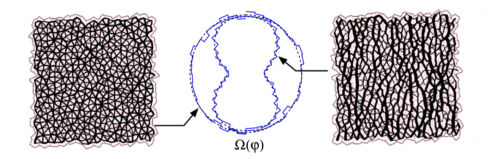
FIG. 4.: The lines show the branch vectors for $\sigma_{1}=\sigma_{3}=160kPa$ (left) and $\sigma_{1}=272kPa$ and $\sigma_{3}=48kPa$ (right). The orientational distribution of branch vectors is shown for both cases.

FIG. 5.: Fabric coefficients of the distribution of the contact normal vectors. They are defined in Eq. (21).

Here $N=N_{0}a_{0}$ is the average coordination number of the polygons, whose initial value $N_{0}=6.0$ reduces as the load is increased. The parameters $a_{0}$, $a_{1}$ and $a_{2}$ can be related respectively to the zeroth, second and fourth order fabric tensor defined in other works to characterize the orientational distribution of the contacts [2, 10]. Here, they will be called fabric coefficients. The dependence of the fabric coefficients on the stress ratio $q/p$ is shown in Fig. 5. We observe that for stress states satisfying $q<0.4p$ there are almost no open contacts. Above this limit a significant number of contacts are open, leading to an anisotropy in the contact network. Fourth order terms in the Fourier expansion are necessary in order to accurately describe this distribution.

B Anisotropic stiffness

We will investigate the effect of the anisotropy of the contact network on the stiffness of the material. The most general linear relation between the incremental stress and the incremental elastic strain for anisotropic materials is given by

$$d\sigma_{ij}=D_{ijkl}d\epsilon^{e}_{kl},$$ (22)

where $D_{ijkl}$ is the stiffness tensor [22]. Since the stress and the strain are symmetric tensors, one can reduce their number of components from $9$ to $6$, and the number of components of the stiffness tensor from $81$ to $36$. Further, by transposing Eq. (22) one obtains that $D_{ijkl}=D_{jilk}$, which reduces the constants from $36$ to $21$. In the particular case of isotropic materials, it has been shown that the number of constants can be reduced to $2$ [22]:

$$d\epsilon^{e}_{ij}=\frac{1}{E}[(1-\nu)d\sigma_{ij}-v\delta_{ij}d\sigma_{kk}].$$ (23)

Here $E$ is the Young modulus and $\nu$ the Poisson ratio. The stress-strain relation of Eq. (22) has been inverted to compare to the elasto-plastic relation of Eq. (19). The description of the general case of the anisotropic elasticity with $21$ constants does not seem trivial. However, since we consider here only plane strain deformations, we can perform further simplifications. We take a coordinate system oriented in the principal stress-strain directions. Thus, the only non-zero components are $d\sigma_{11}\equiv d\sigma_{1}$ and $d\sigma_{33}\equiv d\sigma_{3}$ for the stress and $d\epsilon_{11}\equiv d\sigma_{1}$ and $d\epsilon_{33}\equiv d\sigma_{3}$ for the strain. The anisotropic elastic tensor connecting these components contains only three independent parameters. We can write Eq. (22) as

$$\left[\begin{array}[]{c}d\epsilon^{e}_{1}\\ d\epsilon^{e}_{3}\end{array}\right]=\frac{1}{E}\left[\begin{array}[]{cc}1-\alpha&-\nu\\ -\nu&1+\alpha\end{array}\right]\left[\begin{array}[]{c}d\sigma_{1}\\ d\sigma_{3}\end{array}\right].$$ (24)

The additional parameter $\alpha$ is included here to take into account the anisotropy. When $\alpha=0$, we recover Hooke’s law of Eq. (23). Eq. (19) is calculated from Eq. (24) by performing the transformation in the coordinates of the volumetric strain $de=-d\epsilon_{1}-d\epsilon_{2}$ and deviatoric strain $d\gamma=d\epsilon_{2}-d\epsilon_{1}$, and the pressure $p=(\sigma_{1}+\sigma_{2})/2$ and the deviatoric stress $q=(\sigma_{1}-\sigma_{2})/2$. One obtains:

$$\left[\begin{array}[]{c}de^{e}\\ d\gamma^{e}\end{array}\right]=\frac{2}{E}\left[\begin{array}[]{cc}1-\nu&-\alpha\\ -\alpha&1+\nu\end{array}\right]\left[\begin{array}[]{c}dp\\ dq\end{array}\right]$$ (25)

In the isotropic case $\alpha=0$ this matrix is diagonal. The inverse of the diagonal terms are the bulk modulus $K=E/2(1-\nu)$ and the shear modulus $G=E/2(1+\nu)$. The anisotropy $\alpha\neq 0$ couples the compression mode with the shear deformation such that the compression of the sample will produce deviatoric deformation. This coupling can be observed from the inspection of the elastic part of the strain envelope responses $d\tilde{\epsilon}^{e}(\theta)$ as shown in Fig. 6. For stress values such as $q/p\leq 0.4$ the stress envelope responses collapse on to the same ellipse. This response can be described by Eq. (25) taking $\alpha=0$. For stress values satisfying $q/p>0.4$ there is a coupling between compression and shear deformations and it is necessary to take $\alpha\neq 0$ in Eq. (25).

C Stiffness and fabric

Comparing the calculation of the elastic response in Fig. 6 with the anisotropy of the contact network shown in Fig. 5, a certain correlation is evident between the stiffness tensor and the fabric coefficients of Eq. (21). We observe that Hooke’s law is valid in the regime $q/p<0.4$ where the contact network is isotropic. Moreover, we observe that the opening of the contacts, whose branch vectors are almost perpendicular to the direction of the load, produces a reduction of the stiffness in this direction. This results in an anisotropic elasticity.

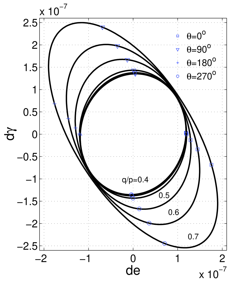
FIG. 6.: Elastic strain envelope responses $d\tilde{\epsilon}^{e}(\theta)$. They are calculated for a pressure $p=160kPa$ and taking deviatoric stresses with $q=0.0p$ (inner), $0.1p$, …,$0.7p$ (outer).

We are going to find a simple relation between the orientational distribution of the contacts and the parameters of the stiffness. These three parameters are calculated from the elastic response by the introduction of the quadratic form of $D^{-1}$:

$$R(\theta)\equiv\hat{\sigma}^{T}D^{-1}\hat{\sigma}=\frac{dp~{}de^{e}+dq~{}d\gamma^{e}}{dp^{2}+dq^{2}}.$$ (26)

Here $\hat{\sigma}^{T}$ is the transpose of $\hat{\sigma}$, which is defined in Eq. (17). This function can be directly obtained from the elastic part of the strain response $d\tilde{\epsilon}^{e}(\theta)$. On the other hand, replacing Eq. (25) in Eq. (26) one can express $R$ in terms of the parameters of the stiffness tensor:

$$R(\theta)=\frac{2}{E}\big{[}1-\nu\cos(2\theta)-\alpha\sin(2\theta)\big{]}.$$ (27)

Using this equation, the parameters $E$, $\nu$ and $\alpha$ are evaluated from the Fourier coefficients of $R$:

$$\frac{1}{E} = \frac{1}{4\pi}\int_{0}^{2\pi}R(\theta)d\theta,$$ (28)

$$\nu = -\frac{E}{2\pi}\int_{0}^{2\pi}R(\theta)\cos(2\theta)d\theta,$$ (29)

$$\alpha = -\frac{E}{2\pi}\int_{0}^{2\pi}R(\theta)\sin(2\theta)d\theta.$$ (30)

Figs. 7, 8 and 9 show the results of the calculation of the Young modulus $E$, the Poisson ratio $\nu$ and the anisotropy factor $\alpha$. Below the limit of isotropy, Hooke’s law can be applied: $E\approx E_{0}$, $\nu\approx\nu_{0}$ and $\alpha\approx 0$. On the other hand, above the limit of isotropy a reduction of the Young modulus is found, along with an increase of the Poisson ratio and the anisotropy factor. In order to evaluate the dependence of these parameters on the fabric coefficients $a_{i}$ from Eq. (21), we introduce an internal variable measuring the degree of anisotropy. This variable is denoted by $a$ and is defined as the percentage change of the total number of contacts.

$$a\equiv\frac{N_{0}-N}{N_{0}}=1-a_{0},$$ (31)

where $a_{0}$ is defined in Eq. (21). The dependence of the parameters of the stiffness tensor on the internal variable $a$ is evaluated by developing the Taylor series around $a=0$:

$$E(a) = E(0)+E^{\prime}(0)a+O\left(a^{2}\right),$$ (32)

$$\alpha(a) = \alpha(0)+\alpha^{\prime}(0)a+O\left(a^{2}\right),$$ (33)

$$\nu(a) = \nu(0)+\nu^{\prime}(0)a+\nu^{\prime\prime}(0)a^{2}+O\left(a^{3}\right).$$ (34)

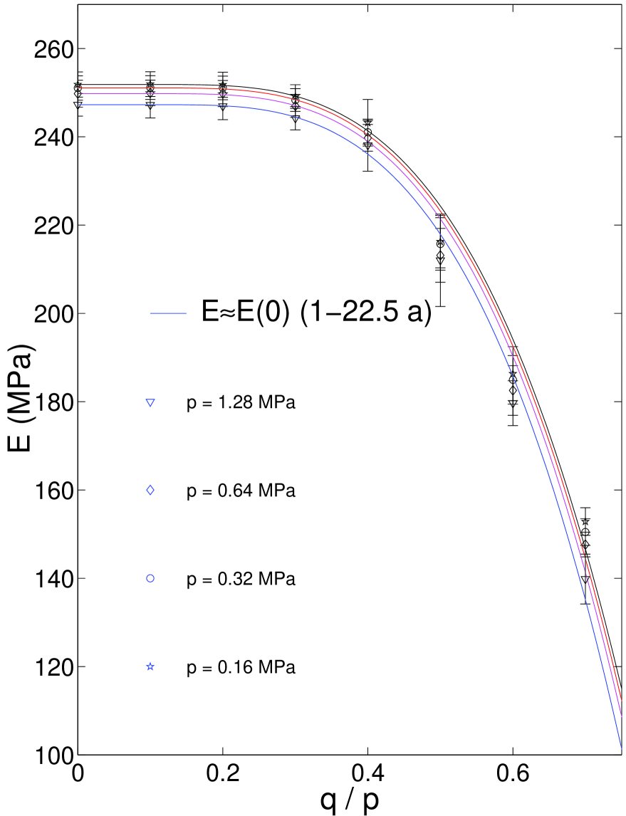
FIG. 7.: Young modulus. The solid line is the linear approximation of $E(d)$. See Eq. (34).

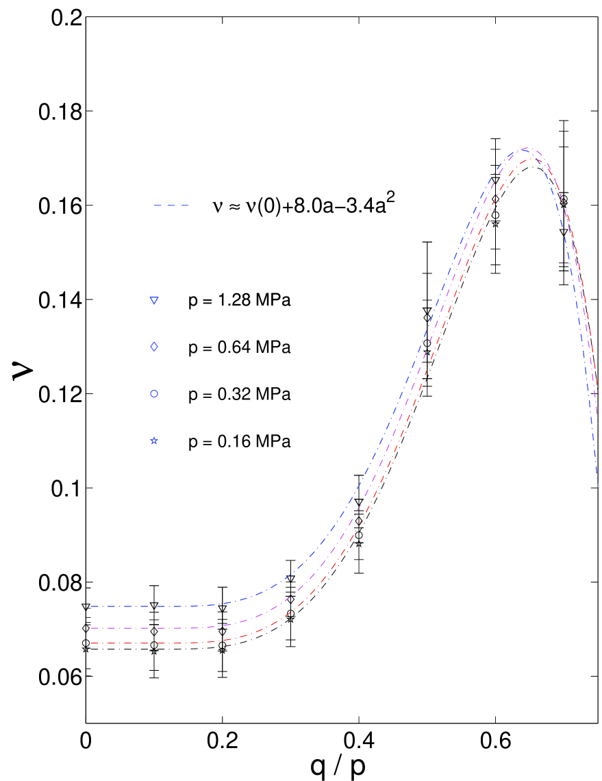
FIG. 8.: Poisson’s ratio. The dashed line is the quadratic approximation of $\nu(d)$. See Eq. (34).

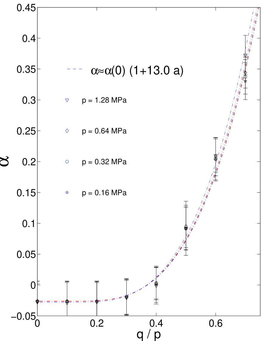
FIG. 9.: Anisotropy parameter. The dashed line is the linear approximation of $\alpha(d)$. See Eq. (34).

The coefficients of this expansion are calculated from the best fit of those expansions. Figs. 7 and 9 show that the linear approximation is good enough to reproduce the Young modulus and the anisotropy factor. The fit of the Poisson ratio, is shown in Fig. 8. The fitting with only one internal variable requires the inclusion of a quadratic approximation. To obtain more accurate relations, it may be necessary to introduce a more complex dependence on the fabric coefficients of Eq. (21).

V Plastic deformations

In the elasto-plastic models of soils the plastic deformation is calculated by introducing a certain number of hypothetical surfaces [25, 26, 27, 18]. In the Drucker-Prager models, the so-called plastic flow rule is calculated from the yield surface and the plastic potential [25, 26, 18]. In the bounding surface plasticity, it is calculated from the loading surface and bounding surfaces [27] We will see that it is possible to calculate the parameters of the flow rule of plasticity, the flow direction, the yield direction and the modulus of plasticity, directly from the stress envelope response $d\tilde{\epsilon}^{p}(\theta)$ without introducing such abstract surfaces.

A Flow rule

In Fig. 3 we found that the plastic envelope response lies almost on a straight line, as is predicted by the Drucker-Prager theory [28]. This motivates us to define the parameters describing the plasticity in the same way as this theory: i.e. the yield direction $\phi$, the flow direction $\psi$, and the plastic modulus $h$.

The yield direction is given by the incremental stress direction $\phi$ with maximal plastic deformation

$$|d\tilde{\epsilon}^{p}(\phi)|=\max_{\theta}{|d\tilde{\epsilon}^{p}(\theta)|},$$ (35)

The flow direction is defined from the orientation of the plastic response at its maximum value

$$\psi=atan2(d\gamma^{p},de^{p})\left|{}_{\theta=\phi}\right.$$ (36)

Here $atan2(y,x)$ is the four quadrant inverse tangent of the real parts of the elements of x and y.( $-\pi<=atan2(y,x)<=\pi$). The plastic modulus is obtained from the modulus of the maximal plastic response.

$$\frac{1}{h}=\frac{|d\tilde{\epsilon}^{p}(\phi)|}{|d\tilde{\sigma}|}.$$ (37)

The incremental plastic response can be expressed in terms of these quantities. Let us define the unitary vectors $\hat{\psi}$ and $\hat{\psi}^{\perp}$. The first one is oriented in the direction of $\psi$ and the second one is the rotation of $\hat{\psi}$ of $90^{o}$. The plastic strain is written as:

$$d\tilde{\epsilon}^{p}(\theta)=\frac{1}{h}\left[\kappa_{1}(\theta)\hat{\psi}+\kappa_{2}(\theta)\hat{\psi}^{\perp}\right],$$ (38)

where the plastic components $\kappa_{1}(\theta)$ and $\kappa_{2}(\theta)$ are given by

$$\kappa_{1}(\theta) = h(d\tilde{\epsilon}^{p}\cdot\hat{\psi})$$ (39)

$$\kappa_{2}(\theta) = h(d\tilde{\epsilon}^{p}\cdot\hat{\psi}^{\perp}).$$ (40)

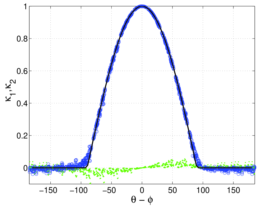
FIG. 10.: Plastic components $\kappa_{1}(\theta)$ (circles) and $\kappa_{2}(\theta)$ (dots). The results for different stress values have been superposed. The solid line represents the truncated cosine function.

These functions are calculated from the resulting plastic response taking different stress values. The results are shown in Fig. 10. We found that the functions $\kappa_{1}(\theta-\psi)$ collapse on to the same curve for all the stress states. This curve fits well to a cosine function, truncated to zero for the negative values. The profile $\kappa_{2}$ depends on the stress ratio we take. This dependency is difficult to evaluate, because the values of this function are of the same order as the statistical fluctuations. In order to simplify the description of the plastic response, the following approximation is made:

$$\kappa_{2}(\theta)\ll\kappa_{1}(\theta)\approx\langle\cos(\theta-\phi)\rangle=\langle\hat{\phi}\cdot\hat{\theta}\rangle,$$ (41)

where $\langle x\rangle\equiv x\Theta(x)$, being $\Theta(x)$ the Heaviside step function. Now, the flow rule results from the substitution of Eqs.(38) and (41) into Eq. (20):

$$d\tilde{\epsilon}^{p}(\theta)=J(\theta)d\tilde{\sigma}=\frac{\langle\hat{\phi}\cdot d\tilde{\sigma}\rangle}{h}\hat{\psi}.$$ (42)

Although we have neither introduced yield functions nor plastic potentials, we recover the same structure of the plastic deformation obtained from the Drucker-Prager analysis [28]. This result suggests the possibility to measure such surfaces directly from the envelope responses without need of an a-priori hypothesis about these surfaces. The next step is to verify the validity of the Drucker-Prager normality postulate, which states that the yield function must coincide with the plastic potential function [28].

B Normality postulate

The Drucker normality postulate was established to describe the plasticity in metals [28]. The question naturally arises as to its validity for the plastic deformation for soils. With this aim, the yield direction and the flow direction have been calculated for different stress states. The results prove that both angles are quite different, as shown in Fig. 11. A large amount of experimental evidence has also indicated a clear deviation from Drucker’s normality postulate [29].

It is not surprising that the Drucker postulate, which has been established for metal plasticity, is not fulfilled in the deformation of granular materials. Indeed, the principal mechanism of plasticity in granular materials is the rearrangement of the grains by the sliding contacts. This is not the case of micro-structural changes in the metals, where there is no frictional resistance [30]. On the other hand, the sliding between the grains can be well handled in the discrete element formulation, which more adequately describes the soil deformation.

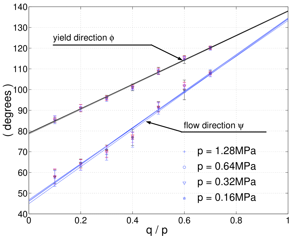
FIG. 11.: The flow direction and the yield direction of the plastic response. Solid lines represent a linear fit.

The fact that the Drucker postulate is not fulfilled in the deformation of the granular materials has led to the so-called non-associated theory of plasticity [18]. This theory introduces a yield surface defining the yield directions and a plastic potential function, which defines the direction of the plastic strain. Both, yield surfaces and plastic potential function can be calculated from the yield and flow direction, which in turn are calculated from the strain envelope response using Eqs. (35) and (36). According to Fig. 11, they follow approximately a linear dependence with the stress ratio $q/p$:

$$\phi = \phi_{0}+\phi^{\prime}_{0}\frac{q}{p},$$ (43)

$$\psi = \psi_{0}+\psi^{\prime}_{0}\frac{q}{p}.$$ (44)

The four parameters $\psi_{0}=46^{o}\pm 0.75^{o}$, $\psi^{\prime}_{0}=88.3^{o}\pm 0.6^{o}$, $\phi_{0}=78.9^{o}\pm 0.2^{o}$ and $\phi^{\prime}_{0}=59.1^{o}\pm 0.4^{o}$ are obtained from a linear fit of the data. This linear dependence with the stress ratio has been shown to fit well with the experimental data in triaxial [31] and biaxial [32] tests on sand. In fact, this implies that the plastic potential function and the yield surfaces have the same shape, independent on the stress level. This is a basic assumption from several constitutive models [25, 26].

From Eq. (44), one can see that there is a transition from contractancy to dilatancy around $q/p=0.5$. This transition is typically observed in dense sand under biaxial loading [26]. A consequence of this linear dependency is that $\psi\neq 0$ when $q=0$. This implies the existence of deviatoric plastic strain when the sample is initially under isotropic loading conditions, which has also been predicted in the original Cam-clay model [25].

The existence of deviatoric plastic deformation under extremely small loading appears to be in contradiction to the fact that the contact network remains isotropic below a certain stress ratio. This matter has also been discussed by Nova [26], who introduced some modifications in the Cam-clay model in order to satisfy the isotropic condition [26]. However, we are going to show from a micro-mechanical inspection that the orientational distribution of the sliding contacts departs from the isotropy for extremely small deviatoric loadings.

C Plasticity & sliding contacts

Under small deformations, the individual grains of a realistic soil behave approximately rigidly, and the plastic deformation of the assembly is due principally to sliding contacts (eventually there is fragmentation of the grains, which is not going to be taken into account here). A complete understanding of soil plasticity is possible, in principle, by the investigation of the micro-mechanical arrangement between the grains. We present here some observations about the anisotropy induced by loading in the subnetwork of the sliding contacts. This investigation will be useful to understand some features of plastic deformation.

The sliding condition at the contacts is given by $|f_{t}|=\mu f_{n}$, where $f_{n}$ and $f_{t}$ are the normal and tangential components of the contact force, and $\mu$ is the friction coefficient. When the sample is isotropically compressed, we observe a significant number of contacts reaching the sliding conditions. If the sample has not been previously sheared, the distribution of the orientation of the branch vectors of all the sliding contacts is isotropic.

This isotropy, however, is broken when the sample is subjected to the slightest deviatoric strain. In effect, at the very beginning of the loading, most of the sliding contacts whose branch vector is oriented nearly parallel to the direction of the loading leave the sliding condition. The anisotropy of the sliding contacts is investigated by introducing the polar function $\Omega^{s}(\varphi)$, where $\Omega^{s}(\varphi)\Delta\varphi$ is the number of sliding contacts per particle whose branch vector is oriented between $\varphi$ and $\varphi+\Delta\varphi$. This can be approximated by a truncated Fourier expansion:

$$\Omega^{s}(\varphi)\approx\frac{N_{0}}{2\pi}\big{[}c_{0}+c_{1}\cos(2\varphi)+c_{2}\cos(4\varphi)\big{]}.$$ (45)

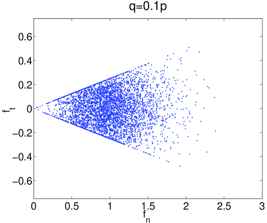
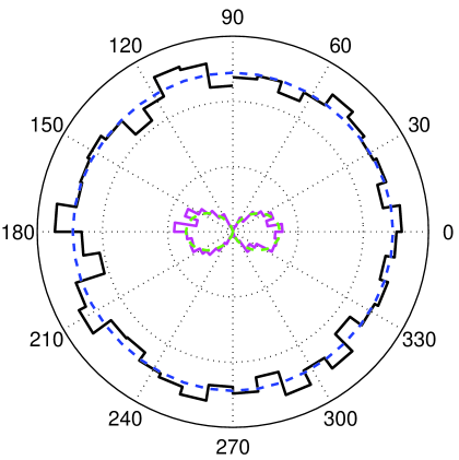
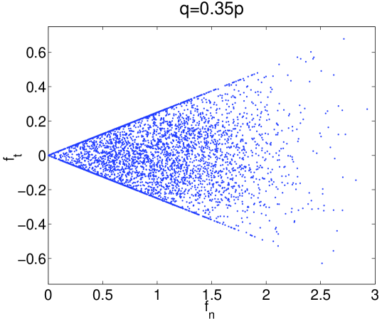
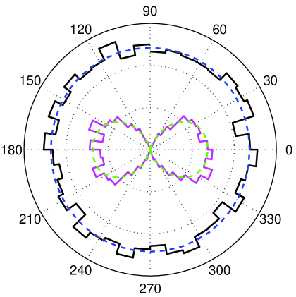
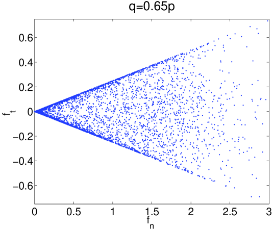
FIG. 12.: Left: force distribution for the stress ratios $q/p=0.1,0.35,0.65$. Here $f_{t}$ and $f_{n}$ are the tangential and normal components of the force. They are normalized by the mean value of $f_{n}$. Right: orientational distribution of the contacts $\Omega(\varphi)$ (outer) and of the sliding contacts $\Omega^{s}(\varphi)$ (inner). $\varphi$ represents the orientation of the branch vector.

Fig. 12 shows the orientational distribution of sliding contacts for different stress ratios. For low stress ratios, the branch vectors $\vec{\ell}$ of the sliding contacts are oriented nearly perpendicular to the loading direction. Sliding occurs perpendicular to $\vec{\ell}$, so in this case it must be nearly parallel to the loading direction. Then, the plastic deformation must be such as $d\epsilon^{p}_{2}\ll d\epsilon^{p}_{1}$, so Eq. (36) yields a flow direction of $\psi\approx 45^{\circ}$, in agreement with Eq. (44).

Increasing the deviatoric strain results in an increase of the number of the sliding contacts. The average of the orientations of the branch vectors with respect to the load direction decreases with the stress ratio, which in turn results in a change of the orientation of the plastic flow. Close to the failure, some of the sliding contacts whose branch vectors are nearly parallel to the loading direction open, giving rise to a butterfly shape distribution, as shown in Fig. 12. In this case, the mean value of the orientation of the branch vector with respect to the direction of the loading is around $\varphi=38^{o}$, which means that the sliding between the grains occurs principally around $52^{o}$ with respect to the vertical. This provides a crude estimate of the ratio between the principal components of the plastic deformation as $d\epsilon^{p}_{2}\approx-d\epsilon^{p}_{1}\tan(52^{o})$. According to Eq. (36) this gives an angle of dilatancy of $\psi=atan2(d\gamma^{p},de^{p})\approx 97^{o}$. This crude approximation is reasonably close to the angle of dilatancy of $103.4^{o}$ calculated from Eq. (44).

A fairly close correlation between the orientation of the sliding contacts and the angle of dilatancy has also been reported by Calvetti et al. [21] using molecular dynamic simulations in triaxial tests. This correlation suggests that the plastic deformation of soils can be micro-mechanically described by the introduction of the fabric constants $c_{i}$ of the equation (45) in the constitutive equations. This investigation would lead to some extensions of the fabric tensor capturing the non-associativity of plastic deformation.

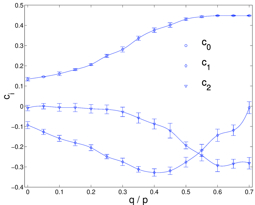
FIG. 13.: Fabric coefficients of the distribution of the contact normal vectors. They are defined in Eq. (45).

D Plastic modulus

The plastic modulus $h$ defined in Eq. (37) is related to the incremental plastic strain in the same way as the Young modulus is related to the incremental elastic strain. Thus, just as we related the Young modulus to the average coordination number of the polygons, it is reasonable to connect $h$ to the fraction of sliding contacts $n_{s}=N_{s}/N$. Here $N$ and $N_{s}$ are the total number of contacts and the number of sliding contacts.

Fig. 14 shows the relation between the hardening and the fraction of the sliding contacts. The results can be fitted to an exponential relation

$$h=h_{o}\exp(-n_{s}/n_{0})$$ (46)

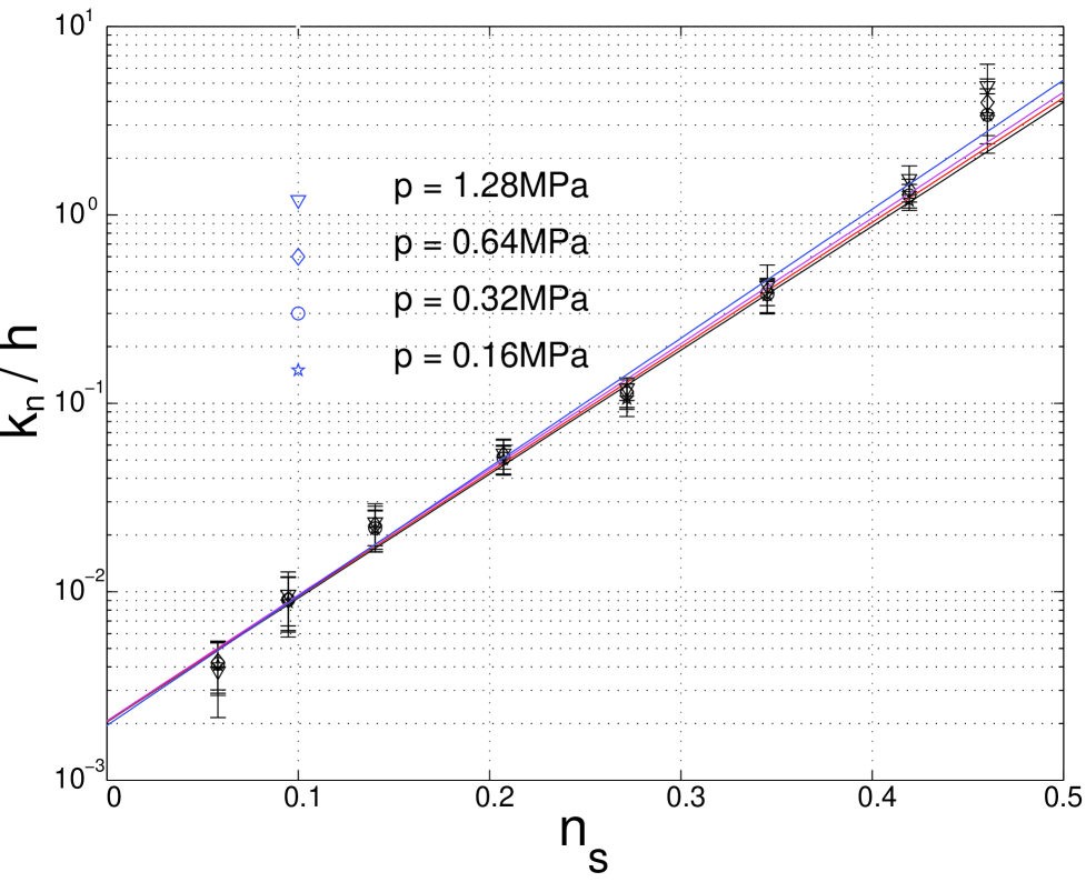
FIG. 14.: Inverse hardening modulus $h$ (MPa) versus fraction of sliding contacts $n_{s}$. The values are taken from $q=0,0.1p,...0.7p$ with different pressures. The lowest value of $n_{s}$ corresponds to $q=0$.

Where $h_{0}=80.0\pm 0.4GPa$ and $n_{0}=0.066\pm 0.002$. This exponential dependence contrasts with the linear relation between the Young modulus and the number of contacts obtained in Sec. IV. From this comparison, it follows that when the number of contacts is such that $n_{s}>n_{0}$, the deformation is not homogeneous, but is principally concentrated more and more around the sliding contacts as their number increases.

The above results suggest that it is possible to establish a dependency of the flow rule on the anisotropy of the subnetwork of the sliding contacts. This relation is more appropriate than just an explicit relation between the flow rule and the stress, which probes to be only valid in the case of monotonic loading [31]. Since the stress can be expressed in terms of micro-mechanical variables, branch vectors and contact forces, the identification of those internal variables measuring anisotropy and force distribution would provide a more general description of the dependence of the flow rule on the history of the deformation.

VI Concluding remarks

The effect of the anisotropy of the contact network on the elasto-plastic response of a Voronoi tessellated sample of polygons has been investigated. The most salient aspects of this anisotropy are summarized as follows:

• The incremental elastic response has a centered ellipse as an envelope response. Below the stress ratio $q/p<0.4$, this response can be described by the two material parameters of Hooke’s law of elasticity: the Young modulus and the Poisson ratio. Above this stress ratio there is a dependence of the stiffness on the stress ratio, which can be connected to the anisotropy induced in the contact network during loading. We should state that this result might be dependent on the preparation procedure. In particular, samples with void ratio different from zero show a smooth transition to the anisotropy, which requires further studies.

• The plastic envelope responses lie almost on the straight line defining the plastic flow direction $\psi$. The yield direction $\psi$ and the plastic modulus $h$ have also been calculated directly from the plastic response. The flow direction and yield direction depend on the stress ratio. In particular, the plastic flow for zero stress ratio has a non-zero deviatoric component suggesting an anisotropy induced for extremely small deviatoric strains. We found that this effect comes from the fact that the sliding contacts depart from anisotropy when the sample is subjected to the smallest deviatoric deformations. We have also shown a correlation between the mean orientation of the sliding contacts and the flow direction of the plastic deformations.

• In the investigation of the connection between the plastic deformation and the number of sliding contacts, we found that the plastic modulus $h$ decays exponentially as the fraction of sliding contacts increases. This contrasts with the linear decrease of the Young modulus $E$ with the increase of the number of open contacts, suggesting that the deformation of the granular assembly is concentrated around the sliding contacts.

Since the mechanical response of the granular sample is represented by a collective response of all the contacts, it is expected that the constitutive relation can be completely characterized by the inclusion of some internal variables, containing the information about the micro-structural arrangements between the grains. We have introduced some internal variables measuring the anisotropy of the contact force network. The fabric coefficients $a_{i}$, measuring the anisotropy of the network of all the contacts, prove to be connected with the anisotropic stiffness. On the other hand, the fabric coefficients $c_{i}$, measuring the anisotropy of the sliding contacts, are related to the plasticity features of the granular materials.

Future work should be oriented towards the elaboration of a theoretical framework connecting the constitutive relation to these fabric coefficients. To provide a complete micro-mechanically based description of the elasto-plastic features, the evolution equations of these internal variables must be included in this formalism. This theory would be an extension of the ideas which have been proposed to relate the fabric tensor to the constitutive relation of granular materials [33, 2, 10].

REFERENCES

- [1] F. Radjai, M. Jean, J. J. Moreau, and S. Roux, Phys. Rev. Lett. 77, 274 (1996).
- [2] C. Thornton and D. J. Barnes, Acta Mechanica 64, 45 (1986).
- [3] S. Luding, R. Tykhoniuk, and A. Thomas, Chem. Eng. Technol. 26, 1229 (2003).
- [4] M. Lätzel, S. Luding, and H. J. Herrmann, Granular Matter 2, 123 (2000), cond-mat/0003180.
- [5] F. Alonso-Marroquin and H. Herrmann, Phys. Rev. Lett. 92, 054301 (2004).
- [6] H. J. Tillemans and H. J. Herrmann, Physica A 217, 261 (1995).
- [7] F. Kun and H. J. Herrmann, Phys. Rev. E 59, 2623 (1999).
- [8] C. Moukarzel and H. J. Herrmann, Journal of Statistical Physics 68, 911 (1992).
- [9] A. Okabe, B. Boots, and K. Sugihara, Spatial Tessellations. Concepts and Applications of Voronoi Diagrams (John Wiley & Sons, Chichester, 1992), wiley Series in probability and Mathematical Statistics.
- [10] M. Lätzel, Ph.D. thesis, Universität Stuttgart, 2002.
- [11] P. A. Cundall and O. D. L. Strack, Géotechnique 29, 47 (1979).
- [12] M. P. Allen and D. J. Tildesley, Computer Simulation of Liquids (Oxford University Press, Oxford, 1987).
- [13] E. Buckingham, Phys. Rev. 4, 345 (1914).
- [14] T. Marcher and P. A. Vermeer, in Continuous and Discontinuous Modelling of Cohesive Frictional Materials (Springer, Berlin, 2001), pp. 89–110.
- [15] K. Bagi, J. Appl. Mech. 66, 934 (1999).
- [16] K. Bagi, Mech. of Materials 22, 165 (1996).
- [17] F. Darve, E. Flavigny, and M. Meghachou, International Journal of Plasticity 11, 927 (1995).
- [18] P. A. Vermeer, in Constitutive Relations of soils (Balkema, Rotterdam, 1984), pp. 175–197.
- [19] H. B. Poorooshasb, I. Holubec, and A. N. Sherbourne, Can. Geotech. J. 4, 277 (1967).
- [20] J. P. Bardet, Int. J. Plasticity 10, 879 (1994).
- [21] F. Calvetti, C. Tamagnini, and G. Viggiani, in Numerical Models in Geomechanics (Swets & Zeitlinger, Lisse, 2002), pp. 3–9.
- [22] L. Landau and E. M. Lifshitz, Theory of Elasticity (Pergamon Press, Moscou, 1986), volume 7 of Course of Theoretical Physics.
- [23] P. A. Cundall, A. Drescher, and O. D. L. Strack, in IUTAM Conference on Deformation and Failure of Granular Materials (Balkema,Rotterdam, Delft, 1982), pp. 355–370.
- [24] A. Drescher and G. de Josselin de Jong, J. Mech. Phys. Solids 20, 337 (1972).
- [25] K. H. Roscoe and J. B. Burland, in Engineering Plasticity (Cambridge University Press, Cambridge, 1968), pp. 535–609.
- [26] R. Nova and D. Wood, Int. J. Num. Anal. Meth. Geomech. 3, 277 (1979).
- [27] Y. F. Dafalias, J. of Engng. Mech 112, 966 (1986).
- [28] D. Drucker and W. Prager, Q. Appl. Math. 10, 157 (1952).
- [29] T. F and K. Ishihara, Soils and Fundations 14, 63 (1974).
- [30] R. Hill, Journal of Geotechnical Engineering 6, 239 (1958).
- [31] P. W. Rowe, Proc. Roy. Soc. A269, 500 (1962).
- [32] M. A. Stroud, Ph.D. thesis, University of Cambridge, 1971.
- [33] R. J. Bathurst and L. Rothenburg, J. Appl. Mech. 55, 17 (1988).