Identifying the maximum entropy method as a special limit
of stochastic analytic continuation

Abstract

The maximum entropy method is shown to be a special limit of the stochastic analytic continuation method introduced by Sandvik [Phys. Rev. B 57, 10287 (1998)]. We employ a mapping between the analytic continuation problem and a system of interacting classical fields. The Hamiltonian of this system is chosen such that the determination of its ground state field configuration corresponds to an unregularized inversion of the analytic continuation input data. The regularization is effected by performing a thermal average over the field configurations at a small fictitious temperature using Monte Carlo sampling. We prove that the maximum entropy method, the currently accepted state of the art, is simply the mean field limit of this fully dynamical procedure. We also describe a technical innovation: we suggest that a parallel tempering algorithm leads to better traversal of the phase space and makes it easy to identify the critical value of the regularization temperature.

I Introduction

Wick rotation transforms imaginary time correlation functions into real, measurable response functions. Analytical results, or numerical results fit to a known functional form, allow for a simple substitution of variables: e.g., $-i\tau\mapsto t(1+i0^{+})$. In general, however, this is not possible. To interpret the results of computer simulations such as quantum Monte Carlo and to make comparisons with experiment, we require a technique that reliably extracts spectral information from imaginary time data. At issue is how best to do this given that the input data is intrinsically noisy and incomplete.

The most widely used technique is the maximum entropy method (MEM), Gull and Skilling (1984); Silver et al. (1990); Gubernatis et al. (1991) which selects the best candidate solution that is consistent with the data. Here, “best” means most likely in the Bayesian sense. There are several variations on the algorithm, but in general it plays out as a competition between the goodness-of-fit measure $\chi^{2}$ and the entropic prior $\mathcal{S}$. In practice, one minimizes the functional $\chi^{2}-\alpha^{-1}\mathcal{S}$ (for some $\alpha^{-1}\neq 0$). The presence of the entropic prior introduces a non-linearity that pulls the minimum away from the least squares solution. One of the key advantages to the method is that it is rigourously derived from statistical considerations and guarantees a unique solution.

Another strategy is to generate a sequence of possible solutions and then take their mean, with the hope that spurious features will be averaged out and legitimate features reinforced (as, e.g., in Ref. Mishchenko et al., 2000). Such methods, however, tend to be ad hoc and are not rigourously justified. There are no criteria for selecting which solutions to include or for assigning their relative weights in the sum. Moreover, how these schemes are related to the MEM solution is unclear. There is no reason a priori to believe that an average over several possible spectra will be closer to the true spectrum than the single most probable one.

Nonetheless, there is compelling evidence that averaging methods can produce better spectra than the MEM. In particular, Sandvik Sandvik (1998) has shown that an unbiased thermal average of all possible spectra, Boltzmann weighted according to $\chi^{2}$, produces (in several test cases) an average spectrum that is in better agreement with the true spectrum (found via exact diagonalization) than is the MEM result. Indeed, our own experience suggests that the MEM is unduly biased toward smooth solutions: sharp spectral features tend to be washed out or obliterated.

In this paper, we show how the averaging approach can be made systematic. We relate the analytic continuation problem to a system of interacting classical fields living on the unit interval and prove that the MEM solution is realized as its mean field configuration. From that point of view, Sandvik’s method amounts to allowing thermal fluctuations about this mean field configuration. It is, in some sense, the most natural dynamical generalization of the MEM. Finally, we sketch out an improved algorithm for performing the stochastic sampling and provide test results for the two methods applied to the spectrum of a simple BCS superconductor.

II Analytic Continuation

A dynamical correlation function of imaginary time, $G(\tau)=\langle\operatorname{T}[\hat{O}(\tau)\hat{O}^{\dagger}(0)]\rangle$, satisfies the (anti-)periodicity relation $G(\tau+\beta)=\mp G(\tau)$, where the upper sign holds for fermionic operators and the lower sign for bosonic ones. Since it is uniquely determined by its values in the region $\tau\in[0,\beta)$, the function admits a discrete Fourier transform

$$G(\tau) =\frac{1}{\beta}\sum_{\omega_{n}}e^{-i\omega_{n}\tau}G(\omega_{n}),$$ (1)

$$G(\omega_{n}) =\int_{0}^{\beta}\!d\tau\,e^{i\omega_{n}\tau}G(\tau),$$ (2)

where the sum is over the Matsubara frequencies $\omega_{n}=(2n+1)\pi/\beta$ for fermions and $\omega_{n}=2n\pi/\beta$ for bosons, with $n\in\mathbb{Z}$.

Provided that $\lvert G(\omega_{n})\rvert$ falls off at least as fast as $1/\lvert\omega_{n}\rvert$ when $n\rightarrow\infty$ (which is guaranteed so long as the operator (anti-)commutator satisfies $\langle\hat{O}\hat{O}^{\dagger}\pm\hat{O}^{\dagger}\hat{O}\rangle<\infty$), the Fourier components are representable in terms of a function of the form

$$\mathcal{G}(z)=\mp\int_{-\infty}^{\infty}\!\frac{d\omega}{2\pi}\frac{\rho(\omega)}{z-\omega}$$ (3)

with the identification $G(\omega_{n})=\mathcal{G}(i\omega_{n})$. The function $\rho(\omega)$ is real-valued and satisfies $\rho(\omega)\geq 0$ for fermions and $\operatorname{sgn}(\omega)\rho(\omega)\geq 0$ for bosons. Note that $\mathcal{G}(z)$ is analytic everywhere in the complex plane, with the possible exception of the real line. Wherever $\rho(\omega)$ is nonzero, there will be a corresponding jump in $\mathcal{G}(z)$:

$$\mathcal{G}(\omega+i0^{+})-\mathcal{G}(\omega-i0^{+})=\pm\rho(\omega).$$ (4)

The principle of analytic continuation states that given the value of $\mathcal{G}(z)$ at a countably infinite number of points along the imaginary axis—by which we mean that $G(\omega_{n})$ or, equivalently, $G(\tau)$ is known—we can uniquely extend $\mathcal{G}(z)$ from those points to the full complex plane. In particular, we can find its values just above and just below the real axis and hence, via Eq. (4), extract $\rho(\omega)$.

According to Eq. (3), we can write

$$G(\omega_{n})=\mp\int\!\frac{d\omega}{2\pi}\frac{\rho(\omega)}{i\omega_{n}-\omega}.$$ (5)

Transforming back to imaginary time, via Eq. (1), and performing the Matsubara frequency sum yields

$$\begin{split}G(\tau)&=\mp\int\!\frac{d\omega}{2\pi}\frac{1}{\beta}\sum_{\omega_{n}}\frac{e^{-i\omega_{n}\tau}}{i\omega_{n}-\omega}\rho(\omega)\\ &=\int\!\frac{d\omega}{2\pi}\frac{e^{-\omega\tau}\rho(\omega)}{e^{-\beta\omega}\pm 1}\\ &=\int\!d\omega\,K(\tau,\omega)A(\omega).\end{split}$$ (6)

In the last line, we have defined

$$K(\tau,\omega)=\begin{cases}e^{-\omega\tau}/(e^{-\beta\omega}+1)&\text{fermions}\\ \omega e^{-\omega\tau}/(e^{-\beta\omega}-1)&\text{bosons}\end{cases}$$ (7)

and

$$A(\omega)=\begin{cases}\rho(\omega)/2\pi&\text{fermions}\\ \rho(\omega)/2\pi\omega&\text{bosons.}\end{cases}$$ (8)

(For some applications it may be more appropriate to define $K(\tau,\omega)=e^{-\omega\tau}$ and $A(\omega)=\rho(\omega)/2\pi(e^{-\beta\omega}-1)$ in the bosonic case.) The spectral function $A(\omega)$, which we shall view as the main quanitity of interest, is positive definite and satisfies a sum rule $\int\!d\omega\,A(\omega)=\mathcal{N}<\infty$.

Equation (6) tells us that we can interpret $G(\tau)$ as a linear functional of $A(\omega)$ with kernel $K(\tau,\omega)$. Hence, the analytic continutation is equivalent to the functional inversion $A(\omega)=\mathbf{K}^{-1}[G(\tau)]$. Only a finite inversion is practicable, however. If we discretize frequency and imaginary time using a uniform mesh (with spacings $\Delta\tau$ and $\Delta\omega$), then $A_{j}=A(\Delta\omega\cdot j)\Delta\omega$ and $G_{k}=G(\Delta\tau\cdot k)$ are related by $A_{j}=\sum_{k}K^{-1}_{jk}G_{k}$. The problem is thus reduced to a matrix inversion of

$$K_{kj}=\frac{e^{\Delta\omega\Delta\tau\cdot j\cdot k}}{e^{-\beta\Delta\omega\cdot j}\pm 1}.$$ (9)

This inversion is not an easy one to perform, however. The condition number of $K_{jk}$ is extremely large: the matrix will have eigenvalues both exponentially large and exponentially small in $\beta$. This means that computation of the inversion requires extremely high numerical precision. Beach and Gooding (2000) Worse, the inversion problem is ill-posed and responds badly to any measurement error in the input set $G_{k}$. The inversion typically overfits the noise with spurious high-frequency modes in $A_{j}$.

The history of practical analytic continuation methods is one of continual refinement of the procedures for regularization of the matrix inversion. The simplest example of regularization is to try

$$A_{j}=\sum_{k}(K_{kj}+\lambda\delta_{kj})^{-1}G_{k}.$$ (10)

Since the high-frequency modes in $A_{j}$ are generated by the smallest eigenvalues of $K_{jk}$, a nonzero value of $\lambda$ will have the effect of suppressing those modes with eigenvalues on the order or $\lambda$ or smaller. To see this, note that for each eigenvalue $E$ of $K_{jk}$, there is an eigenvalue in the inverse matrix that is modified according to $1/E\rightarrow 1/(E+\lambda)$.

This naive scheme has two major flaws. First, filtering out the high frequency modes in this way has the effect of eliminating from the spectral function all fine structure below a certain frequency scale, whether spurious or real. Second, it does not ensure that $A_{j}\geq 0$, as required. The MEM, which we describe briefly in the next section, is considerably more sophisticated about what to filter and has nonnegativity built in.

III Maximum Entropy Method

Suppose that to the exact function $G(\tau)$ we have a measured approximation $\bar{G}(\tau)$. In practice, this will usually have been generated from some Monte Carlo simulation, so that

$$\bar{G}(\tau)=G(\tau)+\text{statistical noise.}$$ (11)

The goodness-of-fit functional

$$\chi^{2}[A]=\int_{0}^{\beta}\!\frac{d\tau}{\sigma(\tau)^{2}}\,\left\lvert\int\!d\omega\,K(\tau,\omega)A(\omega)-\bar{G}(\tau)\right\rvert^{2}$$ (12)

measures how closely the correlation function generated from $A(\omega)$ [via Eq. (6), the forward model] matches $\bar{G}(\tau)$. Here, $\sigma(\tau)$ is the best-guess estimate of the total measurement error in $\bar{G}(\tau)$. (See Appendix A.) There is also an entropy associated with each spectral function,

$$\mathcal{S}[A]=-\int\!d\omega\,A(\omega)\ln\left(A(\omega)/D(\omega)\right),$$ (13)

which measures the information content of $A(\omega)$. Here, $D(\omega)$ is the so-called default model, a smooth function that serves as the zero (maximum) entropy configuration. Any features of the true spectral function known in advance can be encoded in $D(\omega$).

It can be shown that the likelihood of any $A(\omega)$ being the true spectral function is equal to $\mathcal{P}[A]\sim e^{-Q[A]}$ where $Q=\chi^{2}-\alpha^{-1}\mathcal{S}$ (and $\alpha^{-1}$ is a parameter that controls the degree of regularization). The MEM solution corresponds to the spectral function that minimizes $Q$. In practice, the minimization of $Q$ is treated as a numerical optimization problem and is typically performed using the Newton-Raphson algorithm or some other gradient search technique. Nonetheless, a formal solution can be found by identifying the spectral function for which $Q$ is stationary with respect to functional variation. The result, derived in Appendix B, is

$$\bar{A}(\omega)=e^{\alpha\mu}D(\omega)\exp\biggl{[}-2\alpha\int_{0}^{\beta}\!\frac{d\tau}{\sigma(\tau)^{2}}\,\psi(\tau)K(\tau,\omega)\biggr{]}$$ (14)

where

$$\psi(\tau)=\int\!d\omega\,K(\tau,\omega)\bar{A}(\omega)-\bar{G}(\tau)$$ (15)

and $\mu$ is a Lagrange multiplier chosen to enforce the normalization $\int\!d\omega\,A(\omega)=\mathcal{N}$.

In two trivial limits, this set of equations can be solved exactly. When $\alpha\rightarrow\infty$, Eq. (14) demands that $\psi\rightarrow 0$. This yields the noisy, unregularized spectrum $\bar{A}(\omega)=\mathbf{K}^{-1}[\bar{G}(\tau)]$, which is the solution that minimizes $\chi^{2}[A]$ . When $\alpha\rightarrow 0$, $\bar{A}(\omega)=D(\omega)$, the smooth default function. This solution maximizes $\mathcal{S}[A]$. Note that these results come about because $Q\sim\chi^{2}[A]$ and $Q\sim-\mathcal{S}[A]$, respectively, in the two limits.

Over the full range of intermediate values ($0<\alpha<\infty$), Eq. (14) constitutes a one-parameter family of solutions interpolating between these two extremes. An additional condition must be imposed to remove this ambiguity, i.e., to turn the family of solutions into a single final spectrum. In classic MEM, one takes the point of view that somewhere between over-fitting and over-smoothing lies an ideal intermediate range centred on some optimal value of $\alpha$. In other schemes, the final result is produced by averaging, $\bar{A}(\omega)=\int_{0}^{\infty}\!d\alpha\,w(\alpha)\bar{A}(\alpha,\omega)/\int_{0}^{\infty}\!d\alpha\,w(\alpha)$, in which case the question becomes which weighting function $w(\alpha)$ to use. In their definitive review, Jarrell and Gubernatis (1996) Jarrel and Gubernatis address these issues in greater detail.

IV The Stochastic Approach

In this section and the next, we introduce the stochastic analytic continuation approach and demonstrate how it is related to the MEM. To start, consider a smooth mapping $\phi:\mathbb{R}\mapsto[0,1]$, which takes the frequency domain of the spectral function onto the unit interval. Such a function will be of the form

$$\phi(\omega)=\frac{1}{\mathcal{N}}\int_{-\infty}^{\omega}\!d\nu\,D(\nu)$$ (16)

where $D=\mathcal{N}\phi^{\prime}$ is positive definite and (like $A$) normalized to $\mathcal{N}$ but otherwise arbitrary. (We use the notation $D$ for the mapping’s kernel in anticipation of identifying it with the default model of the MEM.) Then,

$$1=\frac{1}{\mathcal{N}}\int\!d\omega\,A(\omega)=\int\!d\phi(\omega)\frac{A(\omega)}{D(\omega)}=\int_{0}^{1}\!dx\,n(x).$$ (17)

In the last line, we have made the change of variables $x=\phi(\omega)$ and introduced the dimensionless field

$$n(x)=\frac{A(\phi^{-1}(x))}{D(\phi^{-1}(x))}$$ (18)

which, according to Eq. (17), is normalized to unity.

Under this change of variables, Eq. (12) becomes

$$H[n(x)]=\int_{0}^{\beta}\!\frac{d\tau}{\sigma(\tau)^{2}}\left\lvert\int_{0}^{1}\!dx\,\hat{K}(\tau,x)n(x)-\bar{G}(\tau)\right\rvert^{2}$$ (19)

with $\hat{K}(\tau,\phi(\omega))=K(\tau,\omega)$. We take the point of view that Eq. (19) is the Hamiltonian for the system of classical fields $\{n(x)\}$. Then, supposing the system is held fixed at a fictitious inverse temperature $\alpha$, it has a partition function $Z=\int\!\mathcal{D}n\,e^{-\alpha H[n]}$ with a measure of integration

$$\int\!\mathcal{D}n=\int_{0}^{\infty}\!\biggl{(}\prod_{x}dn(x)\biggr{)}\delta\biggl{(}\int_{0}^{1}\!dx\,n(x)-1\biggr{)}.$$ (20)

The thermally averaged value of the field is

$$\langle n(x)\rangle=\frac{1}{Z}\int\!\mathcal{D}n\,n(x)e^{-\alpha H[n]}.$$ (21)

The corresponding “thermally regulated” spectral function,

$$\langle{A}(\omega)\rangle=\langle n(\phi(\omega))\rangle D(\omega),$$ (22)

can be recovered using Eq. (18).

At zero temperature ($\alpha\rightarrow\infty$), Eq. (21) simply picks out the ground-state field configuration; the corresponding spectral function is the unregularized analytic continuation result. In the high temperature limit ($\alpha\rightarrow 0$), Eq. (21) represents an unweighted average over all possible field configurations. In that case, the average is completely independent of the input function $\bar{G}(\tau)$ and as such can only yield the zero-information result $\langle n(x)\rangle=1$. From Eq. (18), it follows that $D(\omega)$ is the corresponding spectral function.

These limits are precisely those of the MEM, which we discussed at the end of Sect. III. Note that the kernel of the mapping in Eq. (16) plays the same role as the MEM’s default model and the fictitious temperature the same role as the MEM’s regularization parameter.

V Approximate Solutions

Now let us extend our “interacting classical field” analogy a little further. Expanding the square in Eq. (19), we can cast the Hamiltonian in the familiar form

$$H[n(x)]=\int_{0}^{1}\!dx\,\epsilon(x)n(x)\\ +\frac{1}{2}\int_{0}^{1}\!dx\,dy\,V(x,y)n(x)n(y),$$ (23)

with a free dispersion

$$\epsilon(x)=-2\int_{0}^{\beta}\!\frac{d\tau}{\sigma(\tau)^{2}}\,\bar{G}(\tau)\hat{K}(\tau,x)$$ (24)

and an interaction term

$$V(x,y)=V(y,x)=2\int_{0}^{\beta}\!\frac{d\tau}{\sigma(\tau)^{2}}\,\hat{K}(\tau,x)\hat{K}(\tau,y).$$ (25)

Noninteracting system—Let us ignore the interaction term for a moment and proceed by setting $V=0$. Then, if we represent the delta function constraint in Eq. (20) with an integral representation

$$\delta(X)=\int_{-\infty}^{\infty}\!d\zeta\,\exp\bigl{(}i\zeta X\bigr{)},$$ (26)

the partition function is simply $\mathcal{Z}=\int_{-\infty}^{\infty}\!d\zeta\,e^{-i\zeta}\mathcal{Z}(\zeta)$, where

$$\mathcal{Z}(\zeta)=\int_{0}^{\infty}\!\biggl{(}\prod_{x}dn(x)\biggr{)}e^{-\int_{0}^{1}\!dx\,(\alpha\epsilon(x)-i\zeta)n(x)}.$$ (27)

The saddle point solution for the field is

$$\bar{n}(x)=\frac{\delta}{\delta\epsilon(x)}\biggl{(}-\frac{1}{\alpha}\ln Z(\bar{\zeta})\biggr{)}=e^{-\alpha(\epsilon(x)-\mu)}.$$ (28)

This says that the fields are Maxwell-Boltzmann distributed according to their energy as measured with respect to a chemical potential $\mu\equiv i\bar{\zeta}/\alpha$, which is chosen such that $\int_{0}^{1}\!dx\,\bar{n}(x)=1$.

Mean field treatment—Now let us reintroduce $V$. Assuming that fluctuations of the $n(x)$ field about its mean value are negligible,

$$\bigl{(}n(x)-\bar{n}(x)\bigr{)}\bigl{(}n(y)-\bar{n}(y)\bigr{)}\approx 0,$$ (29)

the Hamiltonian has a mean field form

$$H_{\text{MF}}=\int_{0}^{1}\!dx\,E(x)n(x)+\text{const.},$$ (30)

where

$$E(x)=\frac{\delta H[n]}{\delta n(x)}\biggr{\rvert}_{n=\bar{n}}=\epsilon(x)+\int\!dy\,V(x,y)\bar{n}(y).$$ (31)

Equation (30) leads to the saddle point solution given by Eq. (28) but now with $\epsilon(x)$ replaced by $E(x)$. Using the definition of $E(x)$ from Eq. (31), we arrive at the self-consistent equation

$$\bar{n}(x)=e^{\alpha\mu}\exp\left[-\alpha\Bigl{(}\epsilon(x)+\int\!dy\,V(x,y)\bar{n}(y)\Bigr{)}\right].$$ (32)

Again, $\mu$ is a chemical potential used to fix the normalization.

Now consider the reverse change of variables taking $n(x)$ back to $A(\omega)$. With only a little effort, one can show that Eq. (32) is identical to Eq. (14). What this tells us is that the mean field treatment of the classical field system is formally equivalent to the MEM.

We can make this equivalence more explicit still. The free energy density of the system we have just described is $F=U-\alpha^{-1}S-\mu$, where the internal energy is given by $U=H[\bar{n}(x)]$ and the entropy (see Appendix C) by

$$S[\bar{n}]=-\int_{0}^{1}\!dx\,\bar{n}(x)\ln\bar{n}(x).$$ (33)

As we saw earlier, Eqs. (12) and (19) are connected by a change of variables. Similarly,

$$\begin{split}S[\bar{n}]&=-\int_{0}^{1}\!dx\,\bar{n}(x)\ln\bar{n}(x)\\ &=-\int\!d\phi(\omega)\frac{\bar{A}(\omega)}{D(\omega)}\ln\left(\frac{\bar{A}(\omega)}{D(\omega)}\right)\\ &=-\int\!d\omega\,\bar{A}(\omega)\ln\left(\frac{\bar{A}(\omega)}{D(\omega)}\right)=\mathcal{S}[\bar{A}],\end{split}$$ (34)

where the final equality follows from comparison with Eq. (13). Thus, $\chi^{2}=H[\bar{n}(x)]$ and $\mathcal{S}=S[\bar{n}(x)]$, which makes clear that $F\mathcal{N}=Q=\chi^{2}-\alpha^{-1}\mathcal{S}-\mu\mathcal{N}$. This means that the MEM solution is just the one that minimizes the free energy of the $\{n(x)\}$ system at the mean field level.

VI Monte Carlo Evalutaion

VI.1 Configurations and Update Scheme

The energy of a given field configuration, given by Eq. (19), can be written in the form

$$H[n(x)]=\int_{0}^{\beta}\!d\tau\,h(\tau)^{2},$$ (35)

where

$$h(\tau)=\frac{1}{\sigma(\tau)}\int_{0}^{1}\!dx\,\hat{K}(\tau,x)n(x)-g(\tau)$$ (36)

and $g(\tau)=\bar{G}(\tau)/\sigma(\tau)$ is the input Green’s function rescaled by the variance.

Figure 1: A field configuration of delta functions $n_{C}(x)$ is specified by a set $C=\{r_{\gamma},a_{\gamma}\}$ of residues and coordinates.

Computing $\langle n(x)\rangle$ requires that we integrate over all possible field configurations. To accomplish this, we need some ansatz to render the measure $\mathcal{D}n$ finite. One choice is to represent each field configuration as a superposition of delta functions. In that case, we can parameterize each configuration by a set of residues and coordinates $C=\{r_{\gamma},a_{\gamma}\}$ satisfying $r_{\gamma}>0$, $0\leq a_{\gamma}\leq 1$, and $\sum_{\gamma}r_{\gamma}=1$. The corresponding field configuration is

$$n_{C}(x)=\sum_{\gamma}r_{\gamma}\,\delta(x-a_{\gamma}).$$ (37)

The partition function $\mathcal{Z}=\int dC\,\exp(-\alpha H_{C})$ has a new computationally tractable measure

$$\int\!dC=\prod_{\gamma}\int_{0}^{\infty}\!dr_{\gamma}\int_{0}^{1}\!da_{\gamma}\,\delta\biggl{(}\sum_{\gamma}r_{\gamma}-1\biggr{)}.$$ (38)

In order to calculate the energy $H_{C}$ of a given configuration via Eq. (35), we shall need the relation

$$\begin{split}g(\tau)+h_{C}(\tau)&=\frac{1}{\sigma(\tau)}\int_{0}^{1}\!dx\,\hat{K}(\tau,x)n_{C}(x)\\ &=\frac{1}{\sigma(\tau)}\sum_{\gamma}r_{\gamma}\hat{K}(\tau,a_{\gamma}).\end{split}$$ (39)

Now suppose that the configuration is modified ($C\mapsto C^{\prime}$) by altering the parameters in some subset $\Lambda$ of the delta function walkers:

$$\begin{split}r_{\gamma}\mapsto r^{\prime}_{\gamma}&=r_{\gamma}+\sum_{\lambda\in\Lambda}\delta_{\gamma\lambda}\Delta r_{\lambda},\\ a_{\gamma}\mapsto a^{\prime}_{\gamma}&=a_{\gamma}+\sum_{\lambda\in\Lambda}\delta_{\gamma\lambda}\Delta a_{\lambda}.\end{split}$$ (40)

Accordingly, $h_{C}\mapsto h_{C^{\prime}}=h_{C}+\Delta h$, where

$$\Delta h(\tau)=\frac{1}{\sigma(\tau)}\sum_{\lambda\in\Lambda}\Bigl{[}r^{\prime}_{\lambda}\hat{K}(\tau,a^{\prime}_{\lambda})-r_{\lambda}\hat{K}(\tau,a_{\lambda})\Bigr{]}.$$ (41)

The configuration energy changes to

$$\begin{split}H_{C^{\prime}}&=\int_{0}^{\beta}\!d\tau\,\bigl{(}h_{C}(\tau)+\Delta h(\tau)\bigr{)}^{2}\\ &=H_{C}+\int_{0}^{\beta}\!d\tau\,\Delta h(\tau)\bigl{[}2h_{C}(\tau)+\Delta h(\tau)\bigr{]}.\end{split}$$ (42)

The Monte Carlo procedure is to calculate $H_{C}$ and $h_{C}(\tau)$ for some arbitrary starting configuation $C$ and then update them whenever a walk is accepted. Acceptance is determined according to the usual Metropolis algorithm: create a modified trial configuration and compute its energy shift $\Delta H=H_{C^{\prime}}-H_{C}$ following Eq. (42); choose a random real number $\xi\in[0,1]$; if $\exp(-\alpha\Delta H)>\xi$, accept the walk and update

$$\begin{split}H_{C}&\mapsto H_{C^{\prime}}=H_{C}+\Delta H,\\ h_{C}&\mapsto h_{C^{\prime}}=h_{C}+\Delta h.\end{split}$$ (43)

The path of the delta function walkers through the configuration space must be normalization-conserving and must satisfy detailed balance. Moreover, the entire phase space must, in principle, be accessible. Only two types of moves are necessary to meet these criteria: (1) coordinate shifting moves, in which the walker $\lambda$ is translated by a distance $\Delta a_{\lambda}$, and (2) weight sharing moves, in which the total residue of a subset of walkers is reapportioned amongst themselves such that $\sum_{\gamma}r_{\gamma}=1$ is preserved.

It is useful, however, to introduce additional weight sharing moves that also conserve higher moments

$$\mathcal{M}^{(n)}=\int_{0}^{1}\!dx\,n(x)x^{n}=\sum_{\gamma}r_{\gamma}E_{\gamma}^{n}.$$ (44)

Sandvik has shown that such moves dramatically improve the acceptance ratio of attempted walks at low temperature. At a minimum we want to consider walks that preserve the overall normalization $\mathcal{M}^{(0)}=1$. But we also consider rearrangements of weight between $n>2$ walkers that conserve the first $n-1$ moments. Such a move can be effected as follows. Let $\Lambda=\{\lambda_{1},\lambda_{2},\ldots,\lambda_{n}\}=\{\lambda_{1}\}\cup\tilde{\Lambda}$. Defining the scale factors

$$Q_{\lambda}=\begin{cases}-1&\text{if $\lambda=\lambda_{1}$}\\ \frac{\prod_{\mu\in\tilde{\Lambda}}(a_{\mu}-a_{\lambda_{1}})}{\prod_{\mu\in\tilde{\Lambda}}(a_{\mu}-a_{\lambda})}&\text{if $\lambda\in\tilde{\Lambda}$,}\end{cases}$$ (45)

we can express the changes in residue as

$$r^{\prime}_{\lambda}=r_{\lambda}+\Delta r_{\lambda}=r_{\lambda}-s\,Q_{\lambda},$$ (46)

where $s$ parameterizes the 1-dimensional line of constraint through the $n$-dimensional space of residues. In order to preserve the positivity of the residues, we must impose $r^{\prime}_{\lambda}>0$. Hence, we need to ensure that $r_{\lambda}>Q_{\lambda}\Delta r_{\lambda}$ for all $\lambda\in\Lambda$. Accordingly, we take $s$ to be randomly distributed in the interval

$$\max_{\lambda\in\Lambda^{-}}\bigl{(}r_{\lambda}/Q_{\lambda}\bigr{)}<s<\min_{\lambda\in\Lambda^{+}}\bigl{(}r_{\lambda}/Q_{\lambda}\bigr{)},$$ (47)

where $\Lambda^{-}=\{\lambda:Q_{\lambda}<0\}$ and $\Lambda^{+}=\{\lambda:Q_{\lambda}>0\}$.

VI.2 Parallel Tempering

The Monte Carlo algorithm described above can be improved by introducing parallel tempering. Marinari The idea is to allow multiple instantiations of the simulation to proceed simultaneously for a variety of parameters $\{\alpha_{0},\alpha_{1},\ldots,\alpha_{N}\}$ covering a large range of inverse temperatures. The temperature profile is arbitrary, but we shall find it convenient to choose a constant ratio $\alpha_{p+1}/\alpha_{p}=R$ between one temperature layer and the next.

Most important, the field configurations in each layer are made to evolve in parallel but not independently. Configurations are swapped between adjacent layers in such a way that preserves detailed balance and ensures that each layer $p$ will eventually settle into thermal equilibrium at inverse temperature $\alpha_{p}$. The update rule is quite simple: given two adjacent layers $p$ and $q=p\pm 1$, choose a random real number $\xi\in[0,1]$ and swap the $p$ and $q$ configurations if

$$\exp\Bigl{[}\bigl{(}\alpha_{p}-\alpha_{q}\bigr{)}\bigl{(}H_{p}-H_{q}\bigr{)}\Bigr{]}>\xi.$$ (48)

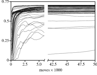
Figure 2: The acceptance ratio of configuration swaps between adjacent levels ($\alpha_{p}\leftrightarrow\alpha_{p+1}$) evolves as a function of the number of updates performed. When the system is fully thermalized, the acceptance ratios stabilize to asymptotic values.

Parallel tempering eliminates the need for a separate, initial annealing stage. Sandvik (1998) Because the simulation simultaneously samples over a large temperature range, there is no danger of getting trapped in false minima: the interlayer walks always provide a cheap pathway between configurations separated by large energy barriers. All that is required is to let the system thermalize for some time before sampling (i.e., before actually beginning to bin and tabulate the field configurations). By tracking the average acceptance rates for swaps between layers, it is straightforward to determine when the system has equilibrated. Figure 2 shows a sample run (for a test case to be described in Sect. VIII). We see that on a stochastic time-scale of several tens of thousands of moves, each temperature layer settles into thermal equilibrium.

An additional advantage of the parallel tempering algorithm is that it yields in one run a complete temperature profile of all the important thermodynamic variables. In the next section, we discuss how we can put that information to use.

VII Critical Temperature

The Monte Carlo simulation yields a set of thermally averaged field configurations $\{\langle n(x)\rangle_{\alpha_{p}}:p=0,1,\ldots N\}$. With little additional effort, we can also keep track of the internal energies $\{U(\alpha_{p})=\langle H[n]\rangle_{\alpha_{p}}:p=0,1,\ldots N\}$. In this section, we propose a final candidate spectral function constructed from only these quantities.

To start, note that the specific heat can be written as

$$C(\alpha_{p})=\frac{dU(\alpha)}{d(\alpha^{-1})}\biggr{\rvert}_{\alpha=\alpha_{p}}\approx\frac{a_{p}U(\alpha_{p})}{\ln R}\frac{d\ln U(\alpha_{p})}{dp}.$$ (49)

(See Appendix D.) In Fig. 3, $\ln U(\alpha_{p})$ is plotted for each temperature level. The knee in the function, occurring in the vicinity of the level $p=p^{*}$, indicates there is a jump in the specific heat. At low temperatures ($\alpha>\alpha^{*}\equiv\alpha_{p*}$), the system freezes out and the correlations $\langle n(x)n(y)\rangle-\langle n(x)\rangle\langle n(y)\rangle$ become short-ranged. There is a characteristic energy scale $E^{*}=U(\alpha^{*})$ associated with this phase transition.

Figure 3: The internal energy of the $\{n(x)\}$ system at each temperature layer is plotted. The knee at $p=p^{*}$, corresponding to a jump in the specific heat, signals a thermodynamic phase transition.

Recall that in the microcanonical ensemble, the average over all configurations having energy $E$ is given by

$$\langle n(x)\rangle_{E}=\int\mathcal{D}n\,n(x)\delta(E-H[n]).$$ (50)

We propose that the final spectrum be defined as

$$\langle\langle n(x)\rangle\rangle=\frac{1}{E^{*}}\int_{0}^{E^{*}}\!dE\,\langle n(x)\rangle_{E},$$ (51)

which sums over all field configurations in the ordered phase (i.e., configurations with energies $E$ satisfying $0\leq E<E^{*}$). Roughly speaking, this amounts to performing an unbiased average over all spectral functions $A$ that surpass the fitting threshold $\chi^{2}[A]<E^{*}$.

Since the Monte Carlo simulation is performed at fixed temperature, however, we must make the change of variables $dE=(dU/d\alpha)d\alpha$. Equation (51) becomes

$$\langle\langle n(x)\rangle\rangle=\frac{1}{U(\alpha^{*})}\int_{\alpha^{*}}^{\infty}\!d\alpha\,\biggl{(}-\frac{dU}{d\alpha}\biggr{)}\langle n(x)\rangle_{\alpha}.$$ (52)

The discretized version of this integral is

$$\langle\langle n(x)\rangle\rangle=\frac{\sum_{p=p^{*}}^{N-1}\bigl{(}U(\alpha_{p})-U(\alpha_{p+1})\bigr{)}\langle n(x)\rangle_{\alpha_{p}}}{U(\alpha_{p^{*}})-U(\alpha_{N})}.$$ (53)

VIII BCS Test Case

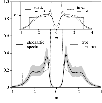
Figure 4: The stochastic analytic continuation method is used to extract the spectrum of a BCS superconductor (bandwidth $W=6$ and gap $2\Delta=1$) from noisy data. The grey region indicates the statistical uncertainty of the computed spectrum. The inset shows the classic and Bryan MEM results.

We showed in Sect. V that the stochastic analytic continuation method is a dynamical generalization of the MEM. The question remains, What is gained by going beyond the mean field calculation? Our contention is that the stochastic method is better able to resolve sharp spectral features buried in noisy data. To illustrate this point, we have taken the spectrum of a BCS superconductor—which contains flat regions, steep peaks, and sharp gap edges—as a test case. The exact spectral function is

$$A(\omega)=\begin{cases}\frac{1}{W}\frac{\lvert\omega\rvert}{\sqrt{\omega^{2}-\Delta^{2}}}&\text{if $\Delta<|\omega|<W/2$}\\ 0&\text{otherwise},\end{cases}$$ (54)

where $W$ is the bandwidth and $2\Delta$ the gap magnitude.

From Eq. (54) we generated an exact $G(\tau)$ using the forward model. We then applied random error to the function to create an approximate $\bar{G}(\tau)$, which was made to serve as the input data for our stochastic algorithm and for two flavours of the MEM—the classic method and a method due to BryanBryan (1990) (both described in Ref. Jarrell and Gubernatis, 1996). Figure 4 shows these computed spectra alongside the exact result.

The most striking aspect of the comparison is that the stochastically generated spectrum does a superior job of modelling the gap. It closely follows the trough of the gap and captures some of the sharpness of the peaks at the gap edges. The MEM spectra, on the other hand, are much too smooth. The classic MEM spectrum is especially poor. It is at best a caricature of the true BCS spectrum: the sharp features are completely washed out and the depression at $\omega=0$ is not a fully developed gap.

Bryan’s algorithm does a somewhat better job of reproducing the gap and its adjacent peaks, but in doing so it also forms a second pair of spurious humps around $\omega=2$. In our experience, this is typical behaviour. The MEM method has trouble making sudden transitions from regions of high to low curvature. What one tends to get is a smooth curve gently oscillating around the correct result. The stochastic method, in contrast, seems to have no trouble generating a flat region next to a sharp peak.

IX Conclusions

In this paper, we have made the case that the MEM is not the best method for extracting spectral information from imaginary time data. Instead, we advocate the use of the stochastic analytic continuation method. Our claim is that the stochastic method is at least as good as the MEM and may even surpass it for a broad class of problems in which the spectrum to be extracted has very sharp features.

This is a difficult point to argue convincingly. New analytic continuation methods tend to face considerable resistance, and claims of superiority on their behalf are met (quite rightly) with a high degree of skepticism. The MEM has a record of years of successful use in a variety of settings; plus, it offers the comfort of a seemingly rock-solid mathematical rationale. Competing schemes tend to lack any clear justification other than a few tantalizing examples of their performance in a handful of test cases.

The prevailing opinion is that the MEM is the definitive “solution” to the analytic continuation problem. Some other method may produce better spectra in particular special cases, but as a general method, the MEM has to win out. The thinking goes: no other algorithm can outperform the MEM because its solution is, by construction, the unique, best candidate spectrum—a claim that rests on the firm foundation of Bayesian logic.

What this line of reasoning misses, however, is the possibility that an average of many likely candidates might better reproduce the true spectral function than does the single most likely spectrum. To give a path integral analogy, we would argue that including fluctuations about a saddle point solution (the single most likely field configuration) can yield a result closer to the full integral. This is how we go about justifying the stochastic analytic continuation method.

Let us be careful about what can be established rigourously. To be precise, the standard conditional probability analysis used to derive the MEM proves only that the most likely spectrum belongs to the family of solutions (parameterized by $\alpha^{-1}$) that minimizes $Q=\chi^{2}-\alpha^{-1}\mathcal{S}$. From our point of view, then, what is required of an averaging method is that it produce at the mean field level a family of solutions that coincides with the MEM result. The stochastic method, as we have formulated it, does exactly this—under the guise of minimizing the free energy $F\mathcal{N}$ $(=Q)$ of a system of classical fields at a fictitious temperature $\alpha^{-1}$.

This correspondence gives us a new way of thinking about the MEM solution. We know that even though a path integral contains jagged, discontinuous field configurations, its saddle point solution is always a smooth, continuous function. This highlights the main deficiency of the MEM—that it fails to model well spectral functions that are not sufficiently smooth—and makes clear why the stochastic method does not suffer from the same limitation.

Another advantage of the stochastic approach is that it helps us to talk about the analytic continuation problem using a more physical language. Having identified the regularization parameter as a temperature, we can ask how the system behaves thermodynamically. The answer, we have suggested, is that the system exhibits ordered and disordered phases that can be interpreted as the good-fitting and ill-fitting regimes. We believe that this gives a much more intuitive picture than does the somewhat obscure probability analysis of the MEM.

We close with a recapitulation of the main results. We have presented a new variant of the stochastic analytic continuation method that differs from Sandvik’s original prescription as follows: as a matter of mathematical formulation, it includes an additional internal freedom that turns out to be equivalent to specifying a default model; as a matter of practical implementation, it is built on a delta function walker scheme and takes advantage of parallel tempering. We have proved that the mean field version of this stochastic method is equivalent to the MEM. Our tests suggest that it outperforms the MEM for spectra with sharp features and fine structure.

Appendix A Statistical Error and Discretization

In Eq. (12), we have used notational shorthand to gloss over two subtle issues. First, we have ignored the fact that the statistical errors between $\bar{G}(\tau)$ and $\bar{G}(\tau^{\prime})$ are not independent for $\tau\neq\tau^{\prime}$. In general, the errors will be positively correlated whenever $\lvert\tau-\tau^{\prime}\rvert$ is sufficiently small. There is also a tendency for them to be negatively (positively) correlated over long-separated times since $G(0^{-})=\mp G(\beta)$ is built in to the definition of the correlation function. Thus, one should more properly write the goodness-of-fit measure as

$$\chi^{2}[A]=\frac{1}{\beta^{2}}\!\int d\tau d\tau^{\prime}\,\Delta(\tau)C^{-1}(\tau,\tau^{\prime})\Delta(\tau^{\prime}),$$ (55)

where $\Delta(\tau)=\int d\omega\,K(\tau,\omega)A(\omega)-\bar{G}(\tau)$ and $C(\tau,\tau^{\prime})$ is the covariance function for $\bar{G}(\tau)$.

Second, we have ignored the discrete nature of the known input data. A Quantum Monte Carlo algorithm, for example, is used to generate stochastically a sequence of independent measurements $\{G^{(1)},G^{(2)},\ldots,G^{(M)}\}$, where each $G^{(m)}$ is an $(L\!\!+\!\!1)$-vector holding the values of the single-particle propagator at imaginary times $\tau_{l}=\beta l/L$ for $l=0,1,\ldots,L$.

The numerical measurement of the Green’s function is accomplished by taking the average

$$\begin{split}\overline{G}_{l}&=\frac{1}{M}\sum_{m=1}^{M}G^{(m)}_{l}.\\ \overline{G_{l}G_{l^{\prime}}}&=\frac{1}{M}\sum_{m=1}^{M}G^{(m)}_{l}G^{(m)}_{l^{\prime}}.\end{split}$$ (56)

The corresponding covariance matrix is given by

$$\begin{split}C_{ll^{\prime}}&=\frac{1}{M\bigl{(}M-1\bigr{)}}\sum_{m=1}^{M}\bigl{(}G^{(m)}_{l}-\bar{G}_{l}\bigr{)}\bigl{(}G^{(m)}_{l^{\prime}}-\bar{G}_{l^{\prime}}\bigr{)}.\\ &=\frac{1}{M-1}\sum_{m=1}^{M}\biggl{[}\overline{G_{l}G_{l^{\prime}}}-\bar{G}_{l}\bar{G}_{l^{\prime}}\biggr{]}\end{split}$$ (57)

Equation (55) must now be discretized in order to make use of Eqs. (56) and (57). The imaginary time integrals are carried out numerically on a uniform mesh of $L$ time slices (spaced by $\Delta\tau=\beta/L$) according to the formula

$$\int_{0}^{\beta}d\tau f(\tau)\approx\sum_{l=0}^{L}\Delta\tau\,w_{l}\,f_{l},$$ (58)

where $f_{l}=f(\Delta\tau\cdot l)$ and the Bode’s rule weights $w_{l}$ satisfy $\sum_{l=0}^{L}w_{l}=L$. Equaton (55) becomes

$$\chi^{2}=\frac{1}{L^{2}}\sum_{l,l^{\prime}=0}^{L}w_{l}\Delta_{l}C^{-1}_{ll^{\prime}}w_{l^{\prime}}\Delta_{l^{\prime}}.$$ (59)

Since $\Delta(0)=\pm\Delta(\beta)$,

$$\chi^{2}=\frac{1}{L^{2}}\sum_{l,l^{\prime}=0}^{L-1}\tilde{w}_{l}\Delta_{l}C^{-1}_{ll^{\prime}}\tilde{w}_{l^{\prime}}\Delta_{l^{\prime}}.$$ (60)

Here, $\tilde{w}_{l}=w_{l}+\delta_{l,0}w_{L}$ for $l=0,1,\ldots L-1$.

We now want to solve for the unitary transformation $U$ that diagonalizes the covariance matrix. This allows us to write $C=U^{t}\Sigma U$ in terms of a set of statistically independent variances $\Sigma=\operatorname{diag}(\sigma^{2}_{1},\sigma^{2}_{2},\ldots,\sigma^{2}_{L})$. The inverse matrix is $C^{-1}=U^{t}\Sigma^{-1}U$.

Putting $C^{-1}_{ll^{\prime}}=\sum_{k=0}^{L}\frac{1}{\sigma^{2}_{k}}U_{kl}U_{kl^{\prime}}$ into Eq. (60) yields

$$\begin{split}\chi^{2}&=\sum_{k=0}^{L}\frac{1}{\sigma^{2}_{k}}\biggl{(}\frac{1}{L}\sum_{l=0}^{L}U_{kl}w_{l}\Delta_{l}\biggr{)}^{2}\\ &=\sum_{k=0}^{L}\frac{1}{\sigma^{2}_{k}}\Bigl{\lvert}(VK)[A]_{k}-(VG)_{k}\Bigr{\rvert}^{2}\end{split}$$ (61)

where we have defined the matrix $V_{kl}=U_{kl}w_{l}/L$.

To recapitulate, the discretization of the $\tau$ integration is implicit in Eq. (12); it also presumes that we are working in the $V$ basis in which the covariance matrix is diagonal.

Appendix B Maximum Entropy Formal Solution

We want to examine the changes in $\mathcal{S}$ with variations in $A(\omega)$. Since the spectral function is subject the the normalization constraint $\int d\omega\,A(\omega)=\mathcal{N}$, variations in $A(x)$ and $A(y)$ for $x\neq y$ are not independent. We can enforce the constraint by introducing a lagrange multiplier $\Gamma=1+\alpha\mu$. Let us define

$$\mathcal{S}[A,\Gamma]\equiv-\int d\omega\,A\ln\left(A/D\right)+\Gamma\int d\omega\,\left(A-D\right).$$ (62)

We have assumed here that $D(\omega)$ and $A(\omega)$ have the same normalization.

Variations of the extended functional, Eq. (62), look like

$$\begin{split}\frac{\delta\mathcal{S}}{\delta A(x)}&=-\ln\left(\frac{A(x)}{D(x)}\right)+\alpha\mu\\ \frac{d\mathcal{S}}{d\mu}&=\alpha\int\!d\omega\,\left(A(\omega)-D(\omega)\right)\end{split}$$ (63)

There is a unique solution that causes these two equations to vanish: $A(x)=D(x)$, $\mu=0$. This implies that $\mathcal{S}=0$ and $\delta\mathcal{S}=0$.

Also, since

$$\frac{\delta^{2}\mathcal{S}}{\delta A(x)\delta A(y)}=-\frac{\delta(x-y)}{A(x)}$$ (64)

we find that $\delta^{2}\mathcal{S}\leq 0$. This means that the entropy functional is strictly non-positive and takes its maximum $\mathcal{S}=0$ when $A$ is equal to the default model.

Similar considerations for $\chi^{2}[A]$ allow us to construct the total variation in $Q=\chi^{2}-\alpha^{-1}\mathcal{S}$. We find that

$$\begin{split}0=\frac{\delta Q[A,\mu]}{\delta A(\omega)}&=2\int_{0}^{\beta}d\tau\,K(\tau,x)\psi(\tau)\\ &\quad-\alpha^{-1}\left[-\ln\left(\frac{A(\omega)}{D(\omega)}\right)+\alpha\mu\right]\end{split}$$ (65)

where

$$\psi(\tau)=\int d\nu\,K(\tau,\nu)A(\nu)-\bar{G}(\tau).$$ (66)

Appendix C Configurational Entropy

Consider a system of $N$ energy levels with degeneracies $m_{p}$ ($p=1,2,\ldots,N$). Suppose that each level is filled with $n_{p}$ indistinguishable particles. The state of the system is unchanged by the rearrangement of particles within a given level. Thus, given a set of occupancies $\{0\leq n_{p}\leq m_{p}\}$, the number of equivalent configurations is $\Omega(\{n_{p}\})=\prod_{p}\begin{pmatrix}m_{p}\\ n_{p}\end{pmatrix}$ and the entropy due to this configuration is

$$\ln\Omega(\{n_{p}\})=\frac{1}{N}\sum_{p}\ln\begin{pmatrix}m_{p}\\ n_{p}\end{pmatrix}.$$ (67)

The binomial coefficient $\begin{pmatrix}m\\ n\end{pmatrix}=m!/(m-n)!/n!$ can be approximated using Stirling’s formula $m!\approx m\ln m$. In the limit of small relative occupancy, this gives

$$\begin{split}\ln\begin{pmatrix}m\\ n\end{pmatrix}&=m\ln m-(m-n)\ln(m-n)-n\ln n\\ &\xrightarrow{m>>n}-n\ln n.\end{split}$$ (68)

Going over to the continuum, we make the identification

$$\begin{split}\frac{1}{N}\sum_{p}&\rightarrow\int\!dx\\ m_{p}&\rightarrow\infty\\ n_{p}&\rightarrow n(x)\end{split}$$ (69)

and use the counting arguments above to write the entropy associated with each field configuration:

$$\ln\Omega[n]=-\int_{0}^{1}\!dx\,n(x)\ln n(x).$$ (70)

The total entropy is

$$S=\int\!\mathcal{D}n\,\ln\Omega[n]\approx\ln\Omega[\bar{n}].$$ (71)

Appendix D Discretization over a logarithmic mesh

Suppose that we want to integrate a function $f(\alpha)$ known only at the points $\alpha_{n}=R^{n}\alpha_{0}$ for $n=0,1,\ldots N$. The integral identity

$$\int\!d\alpha\,f(\alpha)=\int\!d\tilde{\alpha}\,e^{\tilde{\alpha}}f(e^{\tilde{\alpha}})$$ (72)

follows from the change of variables $\alpha=\exp(\tilde{\alpha})$. In this basis, the known points describe a uniform mesh

$$\tilde{\alpha}_{n}=\ln\alpha_{n}=\ln\alpha_{0}+n\ln R$$ (73)

with spacing $\Delta\tilde{\alpha}=\tilde{\alpha}_{n+1}-\tilde{\alpha}_{n}=\ln R$. Accordingly,

$$\begin{split}\int\!d\alpha\,f(\alpha)&\approx\sum_{n=0}^{N}\Delta\tilde{\alpha}\,e^{\tilde{\alpha_{n}}}f(e^{\tilde{\alpha}_{n}})\\ &=\sum_{n=0}^{N}\bigl{(}\ln R\bigr{)}\alpha_{n}f(\alpha_{n}).\end{split}$$ (74)

When the integrand is of the form

$$\frac{dU}{d\alpha}=\frac{1}{e^{\tilde{\alpha}}}\frac{dU}{d\tilde{\alpha}}$$ (75)

we must first discretize the derivative

$$\begin{split}\frac{dU}{d\alpha}\biggr{\rvert}_{\alpha=\alpha_{n}}&\approx\frac{1}{e^{\tilde{\alpha}_{n}}}\frac{U(\alpha_{n+1})-U(\alpha_{n})}{\Delta\tilde{\alpha}}\\ &=\frac{U(\alpha_{n+1})-U(\alpha_{n})}{\alpha_{n}\ln R},\end{split}$$ (76)

which leads to the integrals

$$\int_{\alpha_{p}}^{\alpha_{N-1}}\!d\alpha\,\biggl{(}-\frac{dU}{d\alpha}\biggr{)}\langle n(x)\rangle_{\alpha}\\ \approx\sum_{n=p}^{N-1}\bigl{[}U(\alpha_{n})-U(\alpha_{n+1})\bigr{]}\langle n(x)\rangle_{\alpha_{n}}$$ (77)

and

$$\begin{split}\int_{\alpha_{p}}^{\alpha_{N-1}}\!d\alpha\,\biggl{(}-\frac{dU}{d\alpha}\biggr{)}&\approx\sum_{n=p}^{N-1}\bigl{[}U(\alpha_{n})-U(\alpha_{n+1})\bigr{]}\\ &=U(\alpha_{p})-U(\alpha_{N}).\end{split}$$ (78)

Equation (53) is simply the ratio of these two results.

References

- Silver et al. (1990) R. N. Silver, D. S. Sivia, and J. E. Gubernatis, Phys. Rev. B 41, 2380 (1990).
- Gubernatis et al. (1991) J. E. Gubernatis, M. Jarell, R. N. Silver, and D. S. Sivia, Phys. Rev. B 44, 6011 (1991).
- Gull and Skilling (1984) S. F. Gull and J. Skilling, IEEE Proc. 131, 646 (1984).
- Mishchenko et al. (2000) A. S. Mishchenko, N. V. Prokof’ev, A. Sakamoto, and B. V. Svistunov, Phys. Rev. B 62, 6317 (2000).
- Sandvik (1998) A. W. Sandvik, Phys. Rev. B 57, 10287 (1998).
- Beach and Gooding (2000) K. S. D. Beach and R. J. Gooding, Phys. Rev. B 61, 5147 (2000).
- Jarrell and Gubernatis (1996) M. Jarrell and J. E. Gubernatis, Phys. Rep. 269, 133 (1996).
- (8) E. Marinari, eprint cond-mat/9612010.
- Bryan (1990) R. K. Bryan, Eur. Biophys. J. 18, 165 (1990).