Spin glass models with ferromagnetically biased couplings on the Bethe lattice: analytic solutions and numerical simulations

Abstract

We derive the zero-temperature phase diagram of spin glass models with a generic fraction of ferromagnetic interactions on the Bethe lattice. We use the cavity method at the level of one-step replica symmetry breaking (1RSB) and we find three phases: A replica-symmetric (RS) ferromagnetic one, a magnetized spin glass one (the so-called mixed phase), and an unmagnetized spin glass one. We are able to give analytic expressions for the critical point where the RS phase becomes unstable with respect to 1RSB solutions: we also clarify the mechanism inducing such a phase transition. Finally we compare our analytical results with the outcomes of a numerical algorithm especially designed for finding ground states in an efficient way, stressing weak points in the use of such numerical tools for discovering RSB effects. Some of the analytical results are given for generic connectivity.

I Introduction

Spin glasses are among the most complex models in statistical mechanics that can be treated analytically. Even at the mean field level their solution is highly non-trivial MEPAVI . Moreover when the distribution of the disorder (the distribution of the couplings $J_{ij}$ in the present case) is not symmetric enough, e.g. it has a large positive mean ${\rm E}_{J}[J_{ij}]>0$, the model solution becomes still more complex: Ferromagnetism and spin glass order may coexist in the so-called mixed phase.

The presence of a mixed phase witnesses a very complex energy landscape, with non-trivial thermodynamical properties. Indeed mean-field spin glasses are expected to have a mixed phase, while scaling theories, like the droplet model droplet , do not seem to leave any space for such a phase.

Recently the authors of Ref. KRMA studied numerically ground states of the Edwards-Anderson model with an excess of ferromagnetic couplings in 3d and they found no clear evidence for the existence of a mixed phase. Alternative explanations of their results, compatible with the existence of a mixed phase, are the following: (i) the size of the mixed phase in the 3d EA model may be very tiny; (ii) finite size corrections may be huge and the thermodynamical limit approached very slowly; (iii) consequences of the replica symmetry breaking may be hard to detect in the presence of a strong bias (the global magnetization); (iv) given a large number of quasi-ground-states (with similar energies, but different magnetizations) the numerical algorithm used in Ref. KRMA may have some small bias to find more easily ground states with small magnetization.

In order to shed some more light on the above possible sources of error we believe it is very useful to perform a detailed study of the mixed phase in models where such a study can be done at an analytical level, i.e. models with long-range interactions. From the analytical solution one can extract information on e.g. the size of the mixed phase and the presence of low-energy states with different magnetizations. Moreover, finding ground states with the same algorithm of Ref. KRMA and comparing numerical outcomes with the analytical solution, one can study finite size effects and possible sources of bias in the algorithm.

The complexity of the analytical solution to spin glass models with long-range interactions depends on the interaction topology. Those models where each spin interacts with all the rest of the system (fully-connected topology) can be solved in a compact way thanks to the Parisi ansatz (see e.g. the recent work by Crisanti and Rizzo CrisantiRizzoSK ). On the contrary, the complete solution to those models where each spin interacts only with a finite number of neighbours (Bethe lattice topology) is much more complicated MEPA_bethe : Even the simplest solution with only one step of replica symmetry breaking (1RSB) involves a functional distribution of distributions as the order parameter. Luckily enough such a complex solution can be simplified in some cases: e.g. at zero temperature MEPA_cavityT0 , and when sites are equivalent (factorized solution) FLRZ or when only zero-energy configurations are taken into account CDMM ; MERIZE .

Spin glasses on the Bethe lattice has been extensively studied in the second half of the eighties VianaBray ; MEPA86 ; Kanter ; Kwon ; deDomGold . Unfortunately at that times it was not completely clear how to break the replica symmetry in a way which allow for an analytical treatment: A standard replica calculation for spin glass models on the Bethe lattice would involve an infinite number of overlaps! Until few years ago only replica symmetric (RS) and variational solutions were known for spin glasses on Bethe lattices.

The same definition of “mixed phase” is not clear at the RS level, since it can not be distinguished from a non-homogeneous ferromagnet. Indeed at the RS level only two macroscopic parameters give the full description of the system: the magnetization $m=\sum_{i}m_{i}/N$ and the overlap $q=\sum_{i}m_{i}^{2}/N$, where $m_{i}$ is the local magnetization on site $i$. Given that $q\geq m^{2}$, the only possible RS phases are the following:

• $q=m=0$: paramagnetic phase;

• $q>0$, $m=0$: unmagnetized spin glass phase;

• $q=m^{2}>0\Rightarrow m_{i}=m\;\forall i$: homogeneous ferromagnetic phase;

• $q>m^{2}>0\Rightarrow m_{i}$ depends on the site: Both the non-homogeneous ferromagnetic phase and the mixed phase belong to this class and are thus indistinguishable.

So at the RS level the presence of a mixed phase can only be deduced from the fact that on the RS-to-RSB instability line the magnetization is non-zero, assuming that it does not drop to zero in the RSB phase. The only direct way of observing a mixed phase is to look for RSB solutions with $q>m^{2}>0$: in this case a non-homogeneous ferromagnetic phase corresponds to RS solutions, while a mixed phase to RSB solutions.

In this work we will concentrate on spin glass models with a generic fraction of ferromagnetic interactions defined on Bethe lattices with fixed connectivity. In order to simplify the calculations we will perform a zero-temperature analysis of the ferromagnetic/spin-glass transition at the level of replica symmetric (RS) and one-step replica symmetry breaking (1RSB) solutions.

To our knowledge, the best description of the zero-temperature phase diagram of this model is the one given by Kwon and Thouless Kwon . They used a variational RS approach where the local fields may take any real value. However, in a model having discrete energy levels a real-valued local field is unphysical. Moreover, given that our main aim is the study of the mixed phase in spin glasses, the use of a RSB ansatz is strictly required.

Thanks to the reformulation by Mézard and Parisi MEPA_bethe of the cavity method for finite connectivity models, we are able to derive the correct phase diagram of spin glasses with ferromagnetically biased coupling on the Bethe lattice and to investigate the mixed phase directly with a 1RSB ansatz.

The main questions we would like to answer are the following. Can we locate exactly the boundaries of the mixed phase? How does the size of mixed phase change with the model connectivity? How wide or tiny do we expect to be the mixed phase in the 3d EA model (if any)? What is the physical mechanism inducing the RS to RSB transition? How “strong” are the measurable effects of RBS in the mixed phase? From the numerical point of view, how large are the finite size effects in locating the phase transitions? Is there any bias in the ground states found by the numerical optimization procedure?

The work is organized as follows. In Sec. II we recall model definition and we write cavity self-consistency equations to be solved in Sec. III for Bethe lattices with fixed connectivity 3. There we also compare numerical data to the analytic solution. In Sec. IV we present some result valid for generic connectivity. Finally in Sec. V the answers to questions in the previous paragraph are discussed.

II The model and its solution with the cavity method at zero temperature

We consider a 2-spin interacting spin glass model on a Bethe lattice with fixed connectivity $c=k+1$. The Hamiltonian of the problem is

$$\mathcal{H}=-\sum_{<ij>}J_{ij}\sigma_{i}\sigma_{j}\;,$$ (1)

where $\sigma_{i}=\pm 1$ are Ising variables. The couplings $J_{ij}$ are quenched random variables extracted from the following probability distribution:

$$\mathbf{P}(J)=\frac{1+\rho}{2}\;\delta(J-1)+\frac{1-\rho}{2}\;\delta(J+1)\;.$$ (2)

The parameter $\rho\in[0,1]$ is thus 1 for the ferromagnet and 0 for the unbiased spin glass.

We analyze the problem with the cavity method at zero temperature MEPA_bethe ; MEPA_cavityT0 . The cavity method is based on the analysis of the messages $u$ passed between sites and cavity fields $h$ acting on each site. Following the standard procedure one can write self-consistency equations for the distributions of $u$s and $h$s, that give (if the process converges in the thermodynamic limit) the solution of the model. The basic hypothesis of the above method is the absence of strong correlations between two randomly chosen spins: This is true for Bethe lattice topologies where the typical loop size is of order $\log(N)$, which diverges in the thermodynamic limit $N\rightarrow\infty$.

In this work we use the cavity method at two levels of approximation. The first level corresponds to considering the system with a single thermodynamic pure state, and it is formally equivalent to the Replica Symmetric (RS) approach of the replica method. The second level corresponds to assuming the existence of many equivalent states, which is equivalent to apply the replica method with a one step Replica Symmetry Breaking (1RSB) approximation.

II.1 Self-consistency equations

For models having discrete energy levels, cavity fields at zero temperature only take integer values, since they are related to the difference among energy levels MEPA_cavityT0 . Moreover for the present Hamiltonian, given the cavity field $h$ on a site, the corresponding message sent along the link leaving that site and having coupling $J$ is $u=\text{sign}(Jh)$, with the prescription that $\text{sign}(0)=0$. So for any message we have that $u\in\{-1,0,1\}$.

In the RS case the self-consistency equations are

$$\mathcal{P}(h) = \int\prod_{i=1}^{k}d\mathcal{Q}(u_{i})\;\delta\Big{(}h-\sum_{i=1}^{k}u_{i}\Big{)}\;,$$ (3)

$$\mathcal{Q}(u) = {\rm E}_{J}\int d\mathcal{P}(h)\;\delta\Big{(}u-\text{sign}(Jh)\Big{)}\;,$$ (4)

where ${\rm E}_{J}$ represent the average over the disorder distribution in Eq.(2), and $\mathcal{P}(h)$ [resp. $\mathcal{Q}(u)$] is the probability distribution function (pdf) – over the system – of cavity fields (resp. cavity messages).

The solution to RS equations can be written in terms of the probabilities $p_{0}$, $p_{+}$ and $p_{-}$, defined by

$$\mathcal{Q}(u)=p_{0}\,\delta(u)+p_{+}\,\delta(u-1)+p_{-}\,\delta(u+1)\;,$$ (5)

with the constraint $p_{0}+p_{+}+p_{-}=1$.

Going from the RS to the 1RSB solution MEPA_cavityT0 each field $h_{i}$ (resp. message $u_{i}$) is replaced by a pdf $P_{i}(h)$ [resp. $Q_{i}(u)$] and the order parameters become probability distribution functionals of pdf, $\mathcal{P}[P]$ and $\mathcal{Q}[Q]$.

The 1RSB self-consistency equations are thus

$$\mathcal{P}[P] = \int\prod_{i=1}^{k}D\mathcal{Q}[Q_{i}]\;\delta^{(F)}\Big{[}P-P_{0}[Q_{1},\ldots,Q_{k}]\Big{]}\;,$$ (6)

$$\mathcal{Q}[Q] = {\rm E}_{J}\int D\mathcal{P}[P]\;\delta^{(F)}\Big{[}Q-Q_{0}[P,J]\Big{]}\;,$$ (7)

where $\delta^{(F)}$ is a functional delta and the functions $P_{0}$ and $Q_{0}$ are defined by

$$P_{0}[Q_{1},\ldots,Q_{k}](h) = \frac{1}{A_{k}}\int\prod_{i=1}^{k}dQ_{i}(u_{i})\;e^{-\mu\left(\sum_{i}|u_{i}|-|\sum_{i}u_{i}|\right)}\;\delta\Big{(}h-\sum_{i=1}^{k}u_{i}\Big{)}\;,$$ (8)

$$Q_{0}[P,J](u) = \int dP(h)\;\delta\Big{(}u-\text{sign}(Jh)\Big{)}\;,$$ (9)

where the normalization in Eq.(8) is given by

$$A_{k}[Q_{1},\ldots,Q_{k}]=\int\prod_{i=1}^{k}dQ_{i}(u_{i})\;e^{-\mu\left(\sum_{i}|u_{i}|-|\sum_{i}u_{i}|\right)}\;.$$ (10)

The 1RSB self-consistency equations depend on the “reweighting” parameter $\mu$, which corresponds to the zero temperature limit of the Parisi breaking parameter, $m\simeq\mu T$. The solution to such equations, as well as the corresponding zero-temperature free-energy $\Phi$, will depend on $\mu$.

In full generality one can write the pdf of the message $u_{i}$ as

$$Q_{i}(u_{i})=\eta_{0}^{(i)}\,\delta(u_{i})+\eta_{+}^{(i)}\,\delta(u_{i}-1)+\eta_{-}^{(i)}\,\delta(u_{i}+1)$$ (11)

and describe the pdf $Q_{i}$ by the variables $\eta_{0}^{(i)}$ and $\Delta\eta^{(i)}=\eta_{+}^{(i)}-\eta_{-}^{(i)}$. So the order parameter $\mathcal{Q}[Q]$ becomes the joint pdf $\mathcal{Q}(\eta_{0},\Delta\eta)$. Examples of this distribution can be seen in Fig. 2.

II.2 Free-energy, energy and complexity

Since the RS solution can be formally obtained from the 1RSB one in the $\mu\to 0$ limit, we will write only 1RSB expressions.

The free-energy $\Phi(\mu)$ is composed by two terms MEPA_cavityT0 . The first term, $\Phi_{\rm site}$, is computed merging $c$ messages $u_{i}$, each of them having a pdf $Q_{i}$ randomly extracted from $\mathcal{Q}[Q]$

$$\Phi_{\rm site}(\mu) = -\frac{1}{\mu}\int\prod_{i=1}^{c}D\mathcal{Q}[Q_{i}]\;\log\int\prod_{i=1}^{c}dQ_{i}(u_{i})\;e^{-\mu\left(\sum_{i}|u_{i}|-|\sum_{i}u_{i}|\right)}=$$ (12)

$$= -\frac{1}{\mu}\int\prod_{i=1}^{c}D\mathcal{Q}[Q_{i}]\;\log A_{c}[Q_{1},\ldots,Q_{c}]\;.$$

The second term, $\Phi_{\rm node}$, is computed in the following way (let us write the expression for a generic $p$-spin interaction, being $p=2$ in our case)

$$\Phi_{\rm node}(\mu) = -\frac{{\rm E}_{J}}{\mu}\int\prod_{i=1}^{p}D\mathcal{P}[P_{i}]\;\log\int\prod_{i=1}^{p}dP_{i}(h_{i})\;e^{-2\mu\,\theta(-J\prod_{i}h_{i})}=$$ (13)

$$= -\frac{1}{\mu}\int D\mathcal{P}[P]\,D\mathcal{Q}[Q]\;\log\int dP(h)\,dQ(u)\;e^{-2\mu\,\theta(-hu)}\;,$$

with the prescription $\theta(0)=0$ for the step function $\theta(x)$.

The zero-temperature free-energy is given by a proper combination of the two terms (let us write as before the expression for generic $p$-spin interactions, being $p=2$ in our case)

$$\Phi(\mu)=-\frac{c}{p}+\Phi_{\rm site}(\mu)-\frac{c}{p}(p-1)\Phi_{\rm node}(\mu)\;.$$ (14)

Please note that Eq.(14) gives the right free-energy expression only when it is calculated with $\mathcal{Q}[Q]$ and $\mathcal{P}[P]$ solving the self-consistency equations.

As shown in Ref.MEPA_cavityT0 , the cavity free-energy $\Phi(\mu)$ is the Legendre transform of the complexity or configurational entropy $\Sigma(E)$. Then, in full analogy with replica calculations Monasson , one can write

$$E(\mu) = \partial_{\mu}\Big{[}\mu\,\Phi(\mu)\Big{]}\;,$$ (15)

$$\Sigma(\mu) = \mu\Big{[}E(\mu)-\Phi(\mu)\Big{]}\;.$$ (16)

The complexity curve $\Sigma(E)$ can be obtained as a parametric plot in the $\mu$ parameter. The ground state energy of 1RSB solution is given by the maximum of $\Phi(\mu)$, while threshold state energy is given by the maximum of $E(\mu)$. The solution of the present model in the spin glass phase is expected to have an infinite number of replica symmetry breaking. In such a situation the true threshold energy is certainly lower than its 1RSB approximation.

III Connectivity 3 case ($k=2$)

For the ease of simplicity we will present all the details only in the $k=2$ case, i.e. fixed connectivity 3, where many calculations can be done analytically. We leave for the next Section the results in the generic connectivity case.

III.1 RS solutions

The RS equations (3,4) can be written very easily in the two variables $p_{0}$ and $m_{\rm RS}=p_{+}-p_{-}$ (that is the magnetization of the RS solution)

$$\left\{\begin{array}[]{l}p_{0}=p_{0}^{2}+[(1-p_{0})^{2}-m_{\rm RS}^{2}]/2\\ m_{\rm RS}=\rho(1+p_{0})m_{\rm RS}\end{array}\right.$$ (17)

These equations admit a paramagnetic solution with $p_{0}=1$ and $p_{+}=p_{-}=0$, a spin glass solution with $p_{0}=p_{+}=p_{-}=1/3$, and two ferromagnetic solutions with

$$p_{0}=\frac{1}{\rho}-1\qquad m_{\rm RS}=\pm\sqrt{8-\frac{10}{\rho}+\frac{3}{\rho^{2}}}\;,$$ (18)

that exist only for $\rho>3/4$. The magnetization and the energy of the RS solution are plotted in Fig. 1. From the RS analysis one would predict solely a spin-glass/ferro transition at $\rho_{\rm F}^{\rm RS}=3/4$.

It was already suggested in Ref. Kwon that the RS phase could be unstable for $\rho$ smaller than some $\rho_{\rm RSB}$. Actually the instability seen in Ref. Kwon is from integer to real-valued fields, which is unphysical. Nevertheless this unphysical instability may suggests that a true instability of the RS solution towards RSB solutions could be present.

III.2 1RSB solutions

In order to study the mixed phase, that is the coexistence of spin glass order and ferromagnetic order, the replica symmetry needs to be broken. The mixed phase corresponds to a RSB solution, i.e. $0<\mu<\infty$, with non-zero magnetization, i.e. $\mathcal{Q}[Q(u)]$ not symmetric under the transformation $u\leftrightarrow-u$.

We solve the 1RSB equations (6,7) using a population dynamics algorithm similar to the one used in Ref. MEPA_bethe . We evolve a population of $(\eta_{0},\Delta\eta)$ pairs, representing the joint pdf $\mathcal{Q}(\eta_{0},\Delta\eta)$, until the population becomes stationary. A single evolution step consists in randomly choosing $k=2$ pairs $(\eta_{0}^{(1)},\Delta\eta^{(1)})$ and $(\eta_{0}^{(2)},\Delta\eta^{(2)})$ from the population, and a coupling $J$ randomly with distribution $\mathbf{P}(J)$. Then a new pair $(\eta_{0}^{(0)},\Delta\eta^{(0)})$ is generated and introduced in the population, replacing a randomly selected pair. The expressions for $\eta_{0}^{(0)}$ and $\Delta\eta^{(0)}$ are the following

$$\eta_{0}^{(0)} = \frac{1}{A_{2}}\left[\eta_{0}^{(1)}\eta_{0}^{(2)}+\frac{e^{-2\mu}}{2}\left((1-\eta_{0}^{(1)})(1-\eta_{0}^{(2)})-\Delta\eta^{(1)}\Delta\eta^{(2)}\right)\right]\;,$$ (19)

$$\Delta\eta^{(0)} = \frac{J}{2A_{2}}\left[(1+\eta_{0}^{(1)})\Delta\eta^{(2)}+\Delta\eta^{(1)}(1+\eta_{0}^{(2)})\right]\;,$$ (20)

$$\text{with}\quad A_{2} = 1-\frac{1-e^{-2\mu}}{2}\left((1-\eta_{0}^{(1)})(1-\eta_{0}^{(2)})-\Delta\eta^{(1)}\Delta\eta^{(2)}\right)\;,$$ (21)

The stationary joint pdf $\mathcal{Q}(\eta_{0},\Delta\eta)$ depends on both $\rho$ and $\mu$, giving the following scenario:

• for $\rho>\rho_{\rm RSB}\simeq 0.833$ the system is in a RS ferromagnetic phase;

• for $\rho<\rho_{\rm RSB}$ the RS solution becomes unstable towards RSB solutions;

• the 1RSB solution has a non-zero magnetization as long as $\rho>\rho_{\rm F}^{\rm 1RSB}\simeq 0.715$ (mixed phase) and becomes unmagnetized below $\rho_{\rm F}^{\rm 1RSB}$. In general $\rho_{\rm F}^{\rm 1RSB}<\rho_{\rm F}^{\rm RS}$ holds.

Figure 1: Magnetization (main plot) and energy (inset) of RS and 1RSB solutions as functions of the ferromagnetic bias $\rho$.

In Fig. 1 we show the magnetization and the energy of 1RSB ground states, i.e. those states maximizing $\Phi(\mu)$: the 1RSB full curve leaves the RS dashed curve below $\rho_{\rm RSB}$ and becomes $\rho$-independent below $\rho_{\rm F}^{\rm 1RSB}$. We have checked that our unmagnetized spin glass solution coincides with the one found in previous works MEPA_cavityT0 ; Boettcher .

Considering $\mu$ values different from the one maximizing $\Phi(\mu)$ we can get information also on metastable states. We find that (i) at the same energy level states with different magnetization do exist and (ii) states with higher energy typically have a smaller magnetization.

Figure 2: Probability distributions in the unmagnetized spin-glass (left) and the mixed phase (right).

In Fig. 2 we show the order parameter $\mathcal{Q}(\eta_{0},\Delta\eta)$ for two values of $\rho$, with $\mu$ chosen such as to maximize $\Phi(\mu)$. For $\rho=0.7<\rho_{\rm F}^{\rm 1RSB}$ (unmagnetized spin glass phase) the joint pdf $\mathcal{Q}(\eta_{0},\Delta\eta)$ is symmetric in $\Delta\eta$, that is $\mathcal{Q}(\eta_{0},-\Delta\eta)=\mathcal{Q}(\eta_{0},\Delta\eta)$. For $\rho=0.8>\rho_{\rm F}^{\rm 1RSB}$ (mixed phase) the symmetry in $\Delta\eta$ breaks down and the pdf becomes more dense around one of the bottom corners – the one on the right in this case. The presence of RSB is still clearly manifested by the spread of the points.

For $\rho>\rho_{\rm RSB}$ the system enters the RS ferromagnetic phase and the order parameter $\mathcal{Q}(\eta_{0},\Delta\eta)$ becomes trivial (for this reason we do not show it), either becoming a delta function on the point of coordinates $(p_{0},m_{\rm RS})$, either concentrating on the corners of the triangle, with weights $p_{-}$, $p_{0}$ and $p_{+}$ (from left to right).

Actually we observe that approaching $\rho_{\rm RSB}$ from below the value of $\mu$ maximizing the free energy diverges. As a consequence broad distributions are suppressed and only delta-shaped $Q(u)$ survive. The correct RS limit is thus recovered with $\mu\to\infty$ and $\mathcal{Q}(\eta_{0},\Delta\eta)$ concentrating on the corners.

Figure 3: The complexity $\Sigma$ as a function of $e^{-\mu}$. For each curve, the part corresponding to physical states is the one on the left of the maximum.

Finally we observe in Fig. 3 that, increasing $\rho$ toward $\rho_{\rm RSB}$, the number of states decreases rapidly (please note the logarithmic scale): e.g. for $\rho=0.8$ the maximum of the complexity $\Sigma$ is an order of magnitude smaller than for $\rho=0.72$, and this implies that much larger system sizes have to be used in order to detect numerically the RSB effects.

III.3 Stability of the RS solution

Among the transition points that we have found with the numerical solution of the 1RSB equations, the one in $\rho_{\rm RSB}$ signaling the instability of the RS solution with respect to RSB fluctuation can be calculated analytically.

From the 1RSB order parameter $\mathcal{Q}(\eta_{0},\Delta\eta)$ one can get back the RS solution in 2 ways

$$\mathcal{Q}(\eta_{0},\Delta\eta) \to \mathcal{Q}_{\rm RS}^{(1)}(\eta_{0},\Delta\eta)=\delta(\eta_{0}-p_{0})\,\delta(\Delta\eta-m_{\rm RS})\;,$$ (22)

$$\mathcal{Q}(\eta_{0},\Delta\eta) \to \mathcal{Q}_{\rm RS}^{(2)}(\eta_{0},\Delta\eta)=\frac{1-p_{0}-m_{\rm RS}}{2}\,\delta(\eta_{0})\,\delta(\Delta\eta+1)+$$ (23)

$$\qquad\qquad+\,p_{0}\,\delta(\eta_{0}-1)\,\delta(\Delta\eta)+\frac{1-p_{0}+m_{\rm RS}}{2}\,\delta(\eta_{0})\,\delta(\Delta\eta-1)\;,$$

where $p_{0}$ and $m_{\rm RS}$ satisfy the RS self-consistency equations (17). Our purpose is to analyze RSB fluctuations around the above 2 solutions in close analogy to what has been done recently in Ref. MORI_STAB .

Fluctuations around $\mathcal{Q}_{\rm RS}^{(1)}(\eta_{0},\Delta\eta)$ are always irrelevant. Indeed if we replace the 2 delta function in Eq.(22) with very narrow functions, the variances of these functions evolve through the matrix

$$\left(\begin{array}[]{cc}3p_{0}-1&-m_{\rm RS}\\ \rho\,m_{\rm RS}&\rho(1+p_{0})\\ \end{array}\right)$$ (24)

whose eigenvalues are always less than 1 (in absolute value) as long as $\rho>3/4$. This would imply a RS ferromagnetic phase always stable.

However what we observe numerically is that the RS ferromagnetic state becomes unstable around $\rho_{\rm RSB}\simeq 0.833$, and for $\rho$ slightly below $\rho_{\rm RSB}$ the population is very dense on the top sides of the triangle (see right panel of Fig. 2). This last observation suggested us to study RSB fluctuations around $\mathcal{Q}_{\rm RS}^{(2)}(\eta_{0},\Delta\eta)$ towards a distribution of the following kind

$$\mathcal{Q}(\eta_{0},\Delta\eta)=\mathcal{Q}_{\rm RS}^{(2)}(\eta_{0},\Delta\eta)+\int dx\,\epsilon_{+}(x)\,\delta(\eta_{0}-1+x)\,\delta(\Delta\eta-x)\,+\\ +\int dx\,\epsilon_{-}(x)\,\delta(\eta_{0}-1+x)\,\delta(\Delta\eta+x)\;,$$ (25)

which is concentrated on the corners and on the top sides of the triangle (see pictorial view in Fig.4).

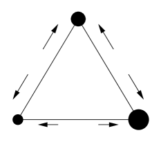
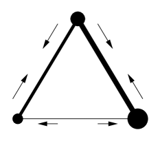
Figure 4: Pictorial view of the 1RSB order parameter above (left) and below (right) the instability point. For $\rho>\rho_{\rm RSB}$ (left) the distribution is concentrated on the three vertices and it is stable under small fluctuations in any direction. For $\rho<\rho_{\rm RSB}$ (right) fluctuations along the upper sides get amplified under the population dynamics.

In terms of pdf $Q_{i}(u)$, the $\mathcal{Q}[Q]$ in Eq.(25) has the following composition

$$Q(u)=\left\{\begin{array}[]{ll}\delta(u)&\text{with prob. }p_{0}\\ \delta(u-1)&\text{with prob. }p_{+}\\ \delta(u+1)&\text{with prob. }p_{-}\\ (1-x)\,\delta(u)+x\,\delta(u-1)&\text{with prob. }\epsilon_{+}(x)\\ (1-x)\,\delta(u)+x\,\delta(u+1)&\text{with prob. }\epsilon_{-}(x)\end{array}\right.$$ (26)

In the following perturbative calculation, the weights on the top sides $\epsilon_{+}(x)$ and $\epsilon_{-}(x)$ will be considered positive and very small: $\epsilon_{+}=\int_{0}^{1}\epsilon_{+}(x)\,dx\ll 1$, $\epsilon_{-}=\int_{0}^{1}\epsilon_{-}(x)\,dx\ll 1$. In order to simplify notation let us use the following short names for the 5 distributions in Eq.(26): $\delta_{0}$, $\delta_{+}$, $\delta_{-}$, $Q_{+}(x)$ and $Q_{-}(x)$.

Our purpose is to calculate how the weights $\epsilon_{+}(x)$ and $\epsilon_{-}(x)$ are modified under one iteration of the population dynamics, given by the expressions in Eqs.(6,7). The only delicate point is the convolution of the $k=2$ pdf $Q_{1}$ and $Q_{2}$ in Eq.(8), that we write in a shorthand notation as $Q_{1}*Q_{2}$. A non-trivial convolution appears only when the messages $u_{1}$ and $u_{2}$ are in contradiction, i.e. when they have different signs. An explicit calculation yields

$$\delta_{+}*Q_{-}(x) = Q_{+}(f_{\mu}(x))\;,$$ (27)

$$\delta_{-}*Q_{+}(x) = Q_{-}(f_{\mu}(x))\;,$$ (28)

$$\text{with}\quad\qquad f_{\mu}(x) = \frac{1-x}{1-(1-e^{-2\mu})\,x}\;.$$ (29)

Please note that, for any finite value of $\mu$, $f_{\mu}$ is a bijective map of the interval $[0,1]$ onto itself, and it has the nice property that $f_{\mu}(f_{\mu}(x))=x$, implying that $\delta_{+}*Q_{-}(f_{\mu}(x))=Q_{+}(x)$.

In a single step of the evolution dynamics, the combinations of parents that produce a distribution $Q_{+}(x)$ in the population of sons are the following: If $J=1$, $\delta_{0}*Q_{+}(x)$ and $\delta_{+}*Q_{-}(f_{\mu}(x))$, and, if $J=-1$, $\delta_{0}*Q_{-}(x)$ and $\delta_{-}*Q_{+}(f_{\mu}(x))$. Analogous expressions for $Q_{-}(x)$ can be obtained with a $+\!\leftrightarrow\!-$ substitution. Each one of these expressions must be multiplied by a combinatorial factor 2. In terms of probabilities we have then

$$\epsilon_{+}(x) = (1+\rho)\Big{[}\;p_{0}\,\epsilon_{+}(x)+p_{+}\,\epsilon_{-}(f_{\mu}(x))\,|f^{\prime}_{\mu}(x)|\;\Big{]}+$$ (30)

$$+ (1-\rho)\Big{[}\;p_{0}\,\epsilon_{-}(x)+p_{-}\,\epsilon_{+}(f_{\mu}(x))\,|f^{\prime}_{\mu}(x)|\;\Big{]}\;,$$

$$\epsilon_{-}(x) = (1+\rho)\Big{[}\;p_{0}\,\epsilon_{-}(x)+p_{-}\,\epsilon_{+}(f_{\mu}(x))\,|f^{\prime}_{\mu}(x)|\;\Big{]}+$$ (31)

$$+ (1-\rho)\Big{[}\;p_{0}\,\epsilon_{+}(x)+p_{+}\,\epsilon_{-}(f_{\mu}(x))\,|f^{\prime}_{\mu}(x)|\;\Big{]}\;.$$

The above expressions hold for continuous functions $\epsilon_{+}(x)$ and $\epsilon_{-}(x)$. In the case these function were made of delta functions, the factors $|f^{\prime}_{\mu}(x)|$ would not appear.

In order to calculate the instability point $\rho_{\rm RSB}$, that is when fluctuations along the top sides become relevant (see Fig. 4), it is enough to consider the total weight on the top sides $\epsilon_{+}$ and $\epsilon_{-}$. Integrating Eqs.(30,31) over $x\in[0,1]$, one can easily obtain an expression for the evolution of the vector $(\epsilon_{+},\epsilon_{-})$, given by the matrix

$$\mathcal{M}=\left(\begin{array}[]{ccc}(1+\rho)p_{0}+(1-\rho)p_{-}&&(1-\rho)p_{0}+(1+\rho)p_{+}\\ (1-\rho)p_{0}+(1+\rho)p_{-}&&(1+\rho)p_{0}+(1-\rho)p_{+}\end{array}\right)\;.$$ (32)

Plugging into $\mathcal{M}$ the values of $p_{0}$, $p_{+}$ and $p_{-}$ corresponding to the RS ferromagnetic solution (18), one finds that the largest eigenvalue (in absolute value) of $\mathcal{M}$ becomes larger than 1 at $\rho_{\rm RSB}=5/6=0.833333$. We have thus found an analytic expression for the instability point seen in the numerical analysis, and the agreement is perfect.

Let us notice en passant that $\rho_{\rm RSB}=5/6$ coincides with the instability point found in Ref. Kwon , where the instability of integer-valued distributions towards real-valued ones was studied . This integers-to-reals instability is quite formal and in principle should not correspond to the physical one. However some other cases have been found MOPARI where such a coincidence can be shown to exist.

Since for $\rho=\rho_{\rm RSB}$ the vector $(\epsilon_{+},\epsilon_{-})$ is an eigenvector of $\mathcal{M}$ with eigenvalue 1, a possible set of solutions to Eqs.(30,31) is given by

$$\epsilon_{+}(x)/\epsilon_{+}=\epsilon_{-}(x)/\epsilon_{-}=S(x)=\sum_{n}a_{n}\Big{[}\delta(x-x_{n})+\delta(x-f_{\mu}(x_{n}))\Big{]}+C(x)\;,$$ (33)

where $C(x)$ is a continuous function such that $C(x)=C(f_{\mu}(x))\,|f^{\prime}_{\mu}(x)|,\;\forall x\in[0,1]$.

It should be then evident that the subspace of functions $S(x)$ which become unstable under the population dynamics for $\rho<\rho_{\rm RSB}$ contains also functions which are very different from those corresponding to the RS solution ($\delta_{0}$, $\delta_{+}$ and $\delta_{-}$), e.g. the function $\delta(x-x^{*}_{\mu})$ with $x^{*}_{\mu}=1/(1+e^{-\mu})$ being the fixed point of the map $f_{\mu}$.

Moreover we observe numerically that the distribution which is actually reached by the population dynamics is very broad, continuous and with no delta functions.

So, in this model, the RSB instability produces an infinitesimal fraction of distributions very different from the RS ones. On this aspect the instability of the present model is different from the one studied in Ref. MORI_STAB for the $p$-spin model. In that case the RS distributions ($\delta_{0}$, $\delta_{+}$ and $\delta_{-}$) acquire a small width, remaining close to the unperturbed ones. We have also studied this last kind of instability, and it turns out that in the present model it becomes relevant only for $\rho<0.8265<\rho_{\rm RSB}$, when the RS solution is already destabilized towards the 1RSB one.

III.4 Comparison with numerical simulations

In order to compare the analytical solution obtained under the 1RSB approximation with numerically computed ground states, we have run an algorithm analogous to the one used to obtain data in Ref. KRMA . More specifically we used the Genetic Renormalization Algorithm of GRA ; it is a heuristic numerical method for computing spin glass ground states with a very high level of reliability. It uses a population based search (thus the name genetic) and applies optimization on multiple scales (thus the name renormalization). We have computed numerically the ground state for Bethe lattices with fixed connectivity 3: system sizes range from $N=64$ to $N=512$, and the number of different sample changes with $N$ in order to keep the statistical error roughly constant. For the size studied here, errors on the ground states energy due to the heuristic are smaller than the statistical errors GRA . Note however that due to the discrete nature of the problem, there is a degeneracy of ground state, so even if we do find a ground state with probability almost $1$, the algorithm may have a natural bias towards some of these ground states, as we shall discuss.

Figure 5: Comparison between the magnetization of ground states found numerically (data with errors) and the analytic prediction under 1RSB (full line) and RS (dotted line) approximations. Statistical errors on numerical data is of the order of symbol size.

In Fig. 5 we compare the analytically computed magnetization (the dotted line is the RS approximation and the full line is the 1RSB approximation) with the magnetization of the ground states found by the numerical algorithm. Numerical data are far from the RS result and are mostly compatible with the 1RSB curve. Nevertheless, deep in the mixed phase ($0.73\lesssim\rho\lesssim 0.76$), we also find evidence that the extrapolation to the thermodynamical limit of the numerically measured magnetization is below the analytical one. This effect actually reduces the size of the mixed phase measured numerically.

A possible explanation to this effect is the following: given a model, like the one we are studying here, which has many degenerate or quasi-degenerate states with different magnetizations, an algorithm looking for such states, starting from a trial configuration of zero magnetization, most probably will stop in a state of magnetization smaller than the typical one. Such an effect has been already observed in Ref. Barthel : in that case a simple algorithm for the search of ground states always found states of zero magnetization in a situation where the thermodynamical magnetization was non-null.

Figure 6: Binder cumulant measured numerically for different system sizes do not cross at the same point, suggesting the presence of strong finite size effects.

We also tried to deduce from the numerical data the critical point $\rho_{\rm F}$ where the magnetization disappears. In Fig. 6 we show the Binder parameter for sizes $N=64,128,256,512$ together with analytical predictions (RS dotted line and 1RSB full line). Increasing $N$, the crossing point moves to left too much in order to be able to do any accurate prediction of $\rho_{\rm F}$. This is a clear evidence that, for this model, finite size effects are huge and make very hard to extract information from numerical data.

Let us stress an important difference between the present model and a similar one with Gaussian coupling, which has been studied in Ref. Liers numerically and analytically at the RS level. The authors of Ref. Liers found that all the numerical results were perfectly compatible, within the statistical error, with the analytic predictions obtained under the RS approximation: for this reason they concluded that RSB effect were tiny in that model. On the contrary here we can clearly see that numerical data are incompatible with the RS results: e.g. the crossing points of Binder cumulant shown in Fig. 6 goes well beyond the RS critical point.

IV Generic connectivity $k+1$

The 1RSB equations can not be solved in a fully analytical form: even in the simplest case ($k=2$) one needs to use a population dynamics algorithm. However we can compute analytically the stability point $\rho_{\rm RSB}$ and the point $\rho_{\rm F}^{\rm RS}$ where the RS solution looses the magnetization.

Let us call $S(k,r)$ the probability of having a field $h=r$ from the sum of $k$ messages $u_{1}\ldots u_{k}$. Its definition is given by the two functions $S_{+}(k,r)=S(k,r)$ and $S_{-}(k,r)=S(k,-r)$ with $r\geq 0$,

$$S_{+}(k,r)=\sum_{q=0}^{\lfloor\frac{k-r}{2}\rfloor}\frac{k!}{q!(r+q)!(k-2q-r)!}\Big{(}\frac{1-p_{0}+m_{\rm RS}}{2}\Big{)}^{r+q}\Big{(}\frac{1-p_{0}-m_{\rm RS}}{2}\Big{)}^{q}p_{0}^{k-2q-r},$$ (34)

$$S_{-}(k,r)=\sum_{q=0}^{\lfloor\frac{k-r}{2}\rfloor}\frac{k!}{q!(r+q)!(k-2q-r)!}\Big{(}\frac{1-p_{0}+m_{\rm RS}}{2}\Big{)}^{q}\Big{(}\frac{1-p_{0}-m_{\rm RS}}{2}\Big{)}^{r+q}p_{0}^{k-2q-r},$$ (35)

where $\lfloor x\rfloor$ is the largest integer not greater than $x$.

For any given $k$, the self-consistency equations thus read

$$p_{0} = S(k,0)\ ,$$ (36)

$$m_{\rm RS} = \rho\sum_{r=1}^{k}\Big{[}S_{+}(k,r)-S_{-}(k,r)\Big{]}\ .$$ (37)

Note that the right hand side of Eq.(37) is always an odd function in the variable $m_{\rm RS}$.

Equations (36,37) admit a paramagnetic solution with $m_{\rm RS}=0$ and $p_{0}=0$, a spin glass solution with $m_{\rm RS}=0$ and $p_{0}=p_{0}^{\rm SG}$, where $p_{0}^{\rm SG}$ is the solution Eq.(36) with $m_{\rm RS}=0$, and a ferromagnetic solution with $m_{\rm RS}\neq 0$ and $p_{0}<p_{0}^{\rm SG}$.

The point $\rho_{\rm F}^{\rm RS}$ where the RS magnetization vanishes can be obtained expanding, for small $m_{\rm RS}$, the right hand side of Eq.(37)

$$m_{\rm RS}=\rho\,c(p_{0},k)\,m_{\rm RS}+\mathcal{O}(m_{\rm RS}^{3})\ ,$$ (38)

and imposing the coefficient to be equal to 1 with $p_{0}=p_{0}^{\rm SG}$, i.e. with the system still unmagnetized: $\rho_{\rm F}^{\rm RS}=1/c(p_{0}^{\rm SG},k)$.

In order to compute the instability point $\rho_{\rm RSB}$, one can proceed as in the previous section. For a generic $k$ the matrix $\mathcal{M}$ reads

$$\mathcal{M}=\left(\begin{array}[]{cc}\frac{1+\rho}{2}Z+\frac{1-\rho}{2}M&\frac{1-\rho}{2}Z+\frac{1+\rho}{2}P\\ \frac{1-\rho}{2}Z+\frac{1+\rho}{2}M&\frac{1+\rho}{2}Z+\frac{1-\rho}{2}P\end{array}\right)$$ (39)

with $Z=k\,S(k-1,0)$, $P=k\,S_{+}(k-1,1)$ and $M=k\,S_{-}(k-1,1)$. The instability point $\rho_{\rm RSB}$ corresponds to the value of $\rho$ for which the maximum eigenvalue of $\mathcal{M}$ becomes larger than 1 in absolute value.

Let us eventually observe that the function $S(k,0)$ is a polynomial in $p_{0}$ with only powers of the same parity of $k$. This implies that, for odd $k$, the solution $p_{0}=0$ always exist, but it is stable under a small perturbation in $p_{0}$ only for $\rho<\rho_{0}$. The stability point $\rho_{0}$ can be easily computed as the value where the coefficient of the linear term in $S(k,0)$ is equal to 1. Analogously to what has been found in $p$-spin models MORI_STAB , we find that for odd $k$ the equality $\rho_{\rm RSB}=\rho_{0}$ always holds.

Figure 7: Left plot: The RSB instability point $\rho_{\rm RSB}$ and the point $\rho_{\rm F}^{\rm RS}$ where the RS solution becomes unmagnetized, as a function of the connectivity $k\!+\!1$. Right plot: rescaled variables.

In Fig. 7 we summarize the values of $\rho_{\rm RSB}$ and $\rho_{\rm F}^{\rm RS}$ for many values of the connectivity $k+1$. It is easy to check that $\rho_{\rm RSB}>\rho_{\rm F}^{\rm RS}$ strictly for any connectivity, and that $\rho_{\rm RSB}\sim\log(k)/\sqrt{k}$ and $\rho_{\rm F}^{\rm RS}\sim 1/\sqrt{k}$ for $k\gg 1$.

For all the values of $\rho$ that we checked, the magnetization of a solution is a non-monotonous function of the reweighting parameter $\mu$. When plotted versus $\exp(-\mu)$ it has a parabolic shape, taking its maximum very close to the value of $\mu$ maximizing $\Phi(\mu)$ and its minima at the extrema $\mu=0$ and $\mu=\infty$ corresponding to the RS solution. So the magnetization in the RSB solutions is typically larger than in the RS solution (see also Fig. 1 for the $k=2$ case). This implies the inequality $\rho_{\rm F}^{\rm 1RSB}\leq\rho_{\rm F}^{\rm RS}$, and the size of the mixed phase is bounded from below by the quantity $(\rho_{\rm RSB}-\rho_{\rm F}^{\rm RS})$, which is strictly positive for any finite connectivity.

We have also checked that in the $k\to\infty$ limit our results converge to those for the SK model SK . Indeed for odd $k$ and $\rho<\rho_{\rm RSB}=\rho_{0}$ the solution has $p_{0}=0$, and the expression for $\rho_{\rm F}^{\rm RS}$ simplifies to

$$\rho_{\rm F}^{\rm RS}=\left[\sum_{i=0}^{(k-1)/2}\frac{k!}{i!(k-i)!}\;\frac{k-2i}{2^{k-1}}\right]^{-1}\quad.$$ (40)

In the $k\to\infty$ limit, $\rho_{\rm F}^{\rm RS}\sim\sqrt{\pi/(2k)}$ which corresponds to the value found by De Almeida and Thouless AT , once the energy of the system is rescaled by the proper $\sqrt{k}$ factor.

Figure 8: The relative size of the mixed phase for a spin glass on the Bethe lattice as a function of the critical temperature. The big black dot is the result for the 3d EA model (after KRMA ).

The authors of Ref. KRMA reported that, if any mixed phase existed in the 3d EA model, its size would be very tiny: defining the relative size as

$$\frac{\rho_{\rm RSB}-\rho_{\rm F}}{(\rho_{\rm RSB}+\rho_{\rm F})/2}\;,$$ (41)

their numerical findings are compatible with a relative size of 0.05 roughly. In order to compare such a numerical result for the 3d EA model with the analytical estimation of the mixed phase found here, we plot in Fig. 8 the relative size of the mixed phase for different connectivities as a function of the critical temperature. The black big point in Fig. 8 corresponds to the numerical result for the 3d EA model. We see clearly that such a numerical finding is perfectly compatible with the mean-field prediction. Again, some 4d simulations are necessary to confirm or infirm the absence of a mixed phase in finite dimensions.

V Summary and discussion

In this work we have studied analytically and numerically the low temperature phase of a spin glass model with ferromagnetically biased couplings defined on a Bethe lattice with fixed connectivity. We have shown that such a model has a mixed phase for any connectivity and that the relative size of such a mixed phase may change a lot with the connectivity. Exact locations of the phase boundaries have been computed numerically and even analytically when possible (e.g. $\rho_{\rm RSB}$ for even connectivity). The instability which induces the spontaneous breaking of the replica symmetry has been deeply analyzed.

Regarding the lack of a clear evidence for a mixed phase in the 3d EA model we have found many reasons for that. Under the Bethe approximation, the expected size of the mixed phase in 3d is very tiny and perfectly compatible to what has been found numerically in Ref. KRMA (see Fig. 8). Finite size corrections on the numerical data are huge (see Fig. 6). Consequences of the RSB may be very hard to detect numerically with small systems: e.g. the complexity in the mixed phase may be very small (see Fig. 3). Finally the same algorithm may have some small bias, whose main effect is to reduce the size of the mixed phase. For all these reasons we believe that the study of the mixed phase is in general, as the study of the spin glass phase in field AT , a very difficult task from the numerical point of view.

Let us finish discussing a point that we believe interesting: the physical meaning of the equality $\rho_{\rm RSB}=\rho_{0}$. For even connectivities the number of cavity messages arriving on a site is an odd number. So the solution with no null messages always exists. It is very curious that the RS-to-RSB instability studied here (as well as the 1RSB-to-2RSB instability studied in Ref. MORI_STAB ) coincides with the appearance of null messages. This coincidence strongly suggests that (for even connectivities) null messages are unphysical and they arise only when the solution ceases to be the correct one. The instability of the 1RSB solution toward further steps of replica symmetry needs to be studied in order to check the above conjecture.

- (1) M. Mézard, G. Parisi, M.A. Virasoro, Spin Glass Theory and Beyond, World Scientific, Singapore (1987)
- (2) A. Bray and M. Moore, J. Phys. C 17, L463 (1984). D. Fisher and D. Huse, Phys. Rev. B 38, 373 (1988).
- (3) F. Krzakala and O.C. Martin, Phys. Rev. Lett. 89, 267202 (2002).
- (4) A. Crisanti, T. Rizzo, Phys. Rev. E 65, 046137 (2002).
- (5) M. Mézard, G. Parisi, Eur. Phys. J. B 20, 217 (2001).
- (6) M. Mézard, G. Parisi, J. Stat. Phys. 111 1 (2003).
- (7) S. Franz, M. Leone, F. Ricci-Tersenghi, and R. Zecchina, Phys. Rev. Lett. 87, 127209 (2001).
- (8) S. Cocco, O. Dubois, J. Mandler, and R. Monasson, Phys. Rev. Lett. 90, 047205 (2003).
- (9) M. Mézard, F. Ricci-Tersenghi, and R. Zecchina, J. Stat. Phys. 111, 505 (2003).
- (10) L. Viana and A.J. Bray, J. Phys. C 18, 3037 (1985).
- (11) M. Mézard and G. Parisi, Europhys. Lett. 3, 67 (1987).
- (12) I. Kanter and H. Sompolinsky, Phys. Rev. Lett. 58, 164 (1987).
- (13) C. Kwon and D.J. Thouless, Phys. Rev. B 37, 7649 (1988).
- (14) C. de Dominicis and Y.Y. Goldschmidt, J. Phys. A 22, L775 (1989).
- (15) R. Monasson, Phys. Rev. Lett. 75, 2847 (1995).
- (16) S. Boettcher, Eur. Phys. J. B 31, 29 (2003).
- (17) A. Montanari and F. Ricci-Tersenghi, Eur. Phys. J. B 33, 339 (2003).
- (18) A. Montanari, G. Parisi, and F. Ricci-Tersenghi, J. Phys. A 37, 2073 (2004).
- (19) J. Houdayer, O. C. Martin, Phys. Rev. Lett. 83 (1999) 1030-1033 and Phys. Rev. E 64, 056704 (2001).
- (20) W. Barthel, A.K. Hartmann, M. Leone, F. Ricci-Tersenghi, M. Weigt, and R. Zecchina, Phys. Rev. Lett. 88, 188701 (2002).
- (21) F. Liers, M. Palassini, A. K. Hartmann and M. Juenger, Phys. Rev. B 68, 094406 (2003).
- (22) D. Sherrington and S. Kirkpatrick, Phys. Rev. Lett. 32 1792 (1975).
- (23) J.R.L. de Almeida and D.J. Thouless, J. Phys. A 11, 983 (1977).