Issues pertaining to D’yakonov-Perel’ spin relaxation in quantum wire channels

Abstract

We elucidate the origin and nature of the D’yakonov-Perel’ spin relaxation in a quantum wire structure, showing (analytically) that there are three necessary conditions for it to exist: (i) transport must be multi-channeled, (ii) there must be a Rashba spin orbit interaction in the wire, and (iii) there must also be a Dresselhaus spin orbit interaction. Therefore, the only effective way to completely eliminate the D’yakonov-Perel’ relaxation in compound semiconductor channels with structural and bulk inversion asymmetry is to ensure strictly single channeled transport. In view of that, recent proposals in the literature that advocate using multi-channeled quantum wires for spin transistors appear ill-advised.

1 Introduction

Coherent spin transport in semiconductor quantum wires is the basis for interesting spintronic devices such as the Spin Field Effect Transistor (SPINFET) [1]. In this device (and its closely related cousins) a quasi one-dimensional quantum “wire” (as opposed to a quasi two-dimensional quantum “well”) is preferred as the channel for several reasons. First, one dimensional confinement of carriers ameliorates the harmful effects of ensemble averaging (at a finite temperature), thereby producing a strong conductance modulation [1]. This is a pre-requisite for any good “transistor” where the conductance of the “on” and “off” states must differ by several orders of magnitude. Second, one-dimensional confinement leads to a severe suppression of spin relaxation [2], [3]. As a result, the transistor channel can be made long, which not only relaxes the demands on fabrication, but also reduces the threshold voltage for switching the device (the threshold voltage of a SPINFET is inversely proportional to the channel length). This, in turn, reduces the dynamic power dissipation. Of course, increasing the gate length also increases the transit time through the channel and the switching delay, but the power dissipation is proportional to the square of the threshold voltage and hence inversely proportional to the square of the gate length, while the transit time is linearly proportional to the gate length. As a result, the important figure of merit – the power delay product – scales inversely with the gate length. A reduced power delay product may be ultimately the most significant advantage that spintronics has over conventional electronics.

This paper is organized as follows. In the next section, we discuss the D’yakonov-Perel’ spin relaxation in a quantum wire structure and derive analytical expressions for the spatial evolution of the average spin of an electron ensemble as a consequence of D’yakonov-Perel’ relaxation. The derived expressions are perfectly general and are valid in the presence of arbitrary driving electric fields, momentum randomizing collisions and inter-subband scattering. Based on these expressions, we derive the necessary and sufficient conditions for the D’yakonov-Perel’ spin relaxation to exist in a quantum wire. Finally, we conclude by stressing the importance of ensuring single channeled transport in spintronic devices in order to eliminate the D’yakonov-Perel’ relaxation.

2 D’yakonov-Perel’ relaxation

The D’yakonov-Perel’ spin relaxation is caused by momentum-dependent spin-orbit interactions that originate from bulk inversion asymmetry (giving rise to a Dresselhaus interaction) and structural inversion asymmetry (giving rise to a Rashba interaction). In this section, we will analytically derive the temporal and spatial evolution of the average spin of an ensemble of electrons in a quantum wire in the presence of these spin orbit interactions. This will elucidate the origin of the D’yakonov-Perel’ relaxation in a quasi one-dimensional structure, and identify pathways to eliminate it.

Consider the quantum wire structure shown in Figure 1. A transverse electric field $E_{y}\hat{y}$ is applied perpendicular to the wire axis ($\hat{x}$) to induce a structural inversion asymmetry that causes a Rashba spin orbit interaction [4]. This structure mimics the SPINFET [1].

Figure 1: Geometry of the quantum wire. Here $E_{x}$ is the longitudinal electric field that induces current flow. The transverse electric field $E_{y}$ induces Rashba spin-orbit coupling.

Since materials that have strong Rashba coupling (preferred for SPINFETs) usually also have bulk inversion asymmetry, we will assume that there is also a Dresselhaus interaction [5].

Spin evolution in the presence of spin-orbit interaction is treated by the standard spin density matrix [6]

$$\rho_{\sigma}(t)=\left[\begin{matrix}\rho\uparrow\uparrow(t)&\rho\uparrow\downarrow(t)\\ \rho\downarrow\uparrow(t)&\rho\downarrow\downarrow(t)\end{matrix}\right]$$ (1)

which is related to the spin polarization component as $S_{n}(t)=Tr[\sigma_{n}\rho_{\sigma}(t)]$ where $n$ = $x$, $y$, $z$ and $\sigma_{n}$-s are Pauli spin matrices. This spin density matrix evolves under the influence of momentum dependent spin orbit coupling Hamiltonian $H_{SO}(\vec{k})$ as

$$\rho_{\sigma}(t+\delta t)=exp\left[-\frac{iH_{SO}(k)\delta t}{\hbar}\right]\rho_{\sigma}(t)\ exp\left[\frac{iH_{SO}(k)\delta t}{\hbar}\right]$$ (2)

The spin-orbit coupling Hamiltonian has two main components: one due to Dresselhaus interaction

$$H_{D}(k)=\gamma\vec{\sigma}\cdot\vec{\kappa}$$ (3)

and the other due to Rashba interaction, whose strength depends on the transverse electric field $E_{y}$ and is given by

$$H_{R}(k)=\eta\left[\vec{\sigma}\times\vec{k}\right]\cdot\hat{y}$$ (4)

The constants $\gamma$ and $\eta$ depend on the material and, in case of $\eta$, also on the external electric field $E_{y}$.

In equation (3), $\vec{\kappa}$ is given by $\vec{\kappa}=\kappa_{x}\hat{x}+\kappa_{y}\hat{y}+\kappa_{z}\hat{z}$ [7] where

$$\kappa_{x}=\frac{1}{2}\left[k_{x}\{\left\langle k_{y}^{2}\right\rangle-\left\langle k_{z}^{2}\right\rangle\}+\{\left\langle k_{y}^{2}\right\rangle-\left\langle k_{z}^{2}\right\rangle\}k_{x}\right]$$ (5)

and $\kappa_{y}$, $\kappa_{z}$ are obtained by cyclic permutations of $k_{x}$, $k_{y}$ and $k_{z}$. In the quantum wire, electrons can move only along $\hat{x}$ (the axis of the quantum wire). Hence setting $k_{y}=k_{z}=0$, the Dresselhaus Hamiltonian simplifies to

$$H_{D}(k)=\gamma\left(\left\langle k_{y}^{2}\right\rangle-\left\langle k_{z}^{2}\right\rangle\right)k_{x}\sigma_{x}$$ (6)

where $\left\langle k_{y}^{2}\right\rangle=\left(n\pi/W_{y}\right)^{2}$ and $\left\langle k_{z}^{2}\right\rangle=\left(m\pi/W_{z}\right)^{2}$. Here $m$ and $n$ are subband indices along $\hat{z}$ and $\hat{y}$, respectively. Also, $W_{y}$ and $W_{z}$ are wire dimensions along $\hat{y}$ and $\hat{z}$ respectively. Similarly, from equation (4) we can derive the Rashba Hamiltonian to be

$$H_{R}(k)=\eta\sigma_{z}k_{x}$$ (7)

From equation (2) we can obtain the temporal evolution of the spin vector as [8], [9]:

$$\frac{d\vec{S}}{dt}=\vec{\Omega}\times\vec{S}$$ (8)

where the precession vector $\vec{\Omega}$ has two orthogonal components $\vec{\Omega}_{R}(k)$ and $\vec{\Omega}_{D}(k)$ due to Rashba and Dresselhaus interactions respectively:

$$\vec{\Omega}_{R}(k)=\frac{2a_{46}}{\hbar}E_{y}k_{x}\hat{z}$$ (9a)

$$\vec{\Omega}_{D}(k)=\frac{2a_{42}}{\hbar}\left[\left(\frac{m\pi}{W_{z}}\right)^{2}-\left(\frac{n\pi}{W_{y}}\right)^{2}\right]k_{x}\hat{x}$$ (9b)

Note that the precession vector $\vec{\Omega}$ lies in the $x-z$ plane (equations (9a) and (9b)).

Figure 2: Axis designations

Now we rotate the $x-z$ plane about the $y$ axis in a way (Figure 2) such that $\vec{\Omega}$ becomes coincident with the new $z$ axis. We name this new $z$ axis $z^{\prime}$ and the new $x$ axis $x^{\prime}$. This requires rotating the $x$ and $z$ axes through an angle $\alpha$ in the $x-z$ plane as shown in Figure 2. The angle $\alpha$ is given by

$$\alpha=tan^{-1}\left(\frac{\Omega_{D}}{\Omega_{R}}\right)$$ (10)

The spin precession equation (8) in the $x^{\prime}yz^{\prime}$ coordinate system reads as follows:

$$\frac{d\vec{S}}{dt}=\vec{\Omega}\times\vec{S}=det\left[\begin{matrix}\hat{x^{\prime}}&\hat{y}&\hat{z^{\prime}}\\ 0&0&\Omega(t)\\ S_{x^{\prime}}(t)&S_{y}(t)&S_{z^{\prime}}(t)\end{matrix}\right]$$ (11a)

where

$$\Omega(t)=\sqrt{\Omega_{D}^{2}(t)+\Omega_{R}^{2}(t)}=\zeta k_{x}(t)$$ (11b)

and

$$\zeta={{2}\over{\hbar}}\sqrt{\left(a_{46}E_{y}\right)^{2}+a_{42}^{2}\left[\left({{m\pi}\over{W_{z}}}\right)^{2}-\left({{n\pi}\over{W_{y}}}\right)^{2}\right]^{2}}$$ (11c)

From equation (11a) we get

$$\frac{dS_{x^{\prime}}}{dt}=-\Omega S_{y}$$ (12a)

$$\frac{dS_{y}}{dt}=\Omega S_{x^{\prime}}$$ (12b)

$$\frac{dS_{z^{\prime}}}{dt}=0$$ (12c)

Figure 3: Spin components in x’yz’ co-ordinate system

In spherical co-ordinates (Figure 3), $S_{x^{\prime}}=S\ sin\ \theta^{\prime}cos\ \phi^{\prime}$, $S_{y}=S\ sin\ \theta^{\prime}sin\ \phi^{\prime}$ and $S_{z^{\prime}}=S\ cos\ \theta^{\prime}$ where $S$ is the magnitude of the spin vector. Substitution of these expressions in equations (12a), (12b) and (12c) yield

$$\frac{d\phi^{\prime}}{dt}=\Omega(t)=\zeta k_{x}(t)$$ (13a)

$$\frac{d\theta^{\prime}}{dt}=0$$ (13b)

Solution of Equation (13a) yields

$$\phi^{\prime}(t)-\phi^{\prime}(0) =\zeta\int_{0}^{t}k_{x}(t^{\prime})dt^{\prime}$$ (14)

$$={{m^{*}\zeta}\over{\hbar}}\int_{0}^{t}v_{x}(t^{\prime})dt^{\prime}$$

$$={{m^{*}\zeta}\over{\hbar}}x$$

$$\equiv\Phi^{\prime}(x)$$

where we have assumed a parabolic electron energy dispersion so that the velocity is given by $v_{x}(t)$ = $\hbar k_{x}(t)/m^{*}$ ($m^{*}$ is the effective mass). Before we proceed to derive the expressions for the spin components as a function of position $x$, we need to relate the primed quantities to their unprimed counterparts.

$$cos\ \theta^{\prime} =\frac{\vec{S}\cdot\hat{z}^{\prime}}{|\vec{S}||\hat{z}^{\prime}|}$$ (15)

$$=(S_{x}/S)\ z^{\prime}_{x}+(S_{y}/S)\ z^{\prime}_{y}+(S_{z}/S)\ z^{\prime}_{z}$$

$$=(S_{x}/S)\ sin\ \alpha+(S_{z}/S)\ cos\ \alpha$$

$$=cos\ \phi\ sin\ \theta\ sin\ \alpha+cos\ \theta\ cos\ \alpha$$

where $z^{\prime}_{x}$ = $sin\ \alpha$, $z^{\prime}_{y}$ = 0 and $z^{\prime}_{z}$ = $cos\ \alpha$. From the above, we find

$$sin\ \theta^{\prime}=\left[1-A\right]^{1/2}$$ (16)

where

$$A =cos^{2}\theta^{\prime}$$ (17)

$$=\left(\frac{S_{x}}{S}\right)^{2}sin^{2}\alpha+\left(\frac{S_{z}}{S}\right)^{2}cos^{2}\alpha+\frac{S_{x}S_{z}}{S^{2}}\ sin\ 2\alpha$$

The components of $\vec{S}$ in the original system of coordinates $(x,y,z)$ are then easily obtained from the components in the primed system $(x^{\prime},y,z^{\prime})$.

$$S_{x} =S_{x^{\prime}}\ cos\ \alpha+S_{z^{\prime}}\ sin\ \alpha$$ (18)

$$=S\ sin\ \theta^{\prime}cos\ \phi^{\prime}\ cos\ \alpha+S\ cos\ \theta^{\prime}sin\ \alpha$$

$$S_{y} =S_{y^{\prime}}=S\ sin\ \theta^{\prime}sin\ \phi^{\prime}$$

$$S_{z} =-S_{x^{\prime}}\ sin\ \alpha+S_{z^{\prime}}\ cos\ \alpha$$

$$=-S\ sin\ \theta^{\prime}cos\ \phi^{\prime}\ sin\ \alpha+S\ cos\ \theta^{\prime}cos\ \alpha$$

Using equations (15)–(18), we get

$$S_{x}(x) =S_{0}\ cos\ [\Phi^{\prime}(x)+\phi^{\prime}(0)]\ cos\ \alpha+S_{x}(0)\ sin^{2}\alpha$$ (19)

$$+S_{z}(0)\ sin\ \alpha\ cos\ \alpha$$

$$S_{y}(x) =S_{0}\ sin\ [\Phi^{\prime}(x)+\phi^{\prime}(0)]$$

$$S_{z}(x) =-S_{0}\ cos\ [\Phi^{\prime}(x)+\phi^{\prime}(0)]\ sin\ \alpha$$

$$+S_{x}(0)\ sin\ \alpha\ cos\ \alpha+S_{z}(0)\ cos^{2}\ \alpha$$

where

$$S_{0}^{2} =S^{2}-S_{x}(0)^{2}sin^{2}\alpha-S_{z}(0)^{2}cos^{2}\alpha$$ (20)

$$-S_{x}(0)\ S_{z}(0)\ sin\ 2\alpha$$

Let us now consider the situation where electrons are injected into the quantum wire with their spins polarized along the $+\hat{x}$ direction. In that case, $\phi^{\prime}(0)=0$, $S$ = $S_{x}(0)$ and $S_{y}(0)=S_{z}(0)$ = 0. The above equation then simplifies to

$$S_{x}(x) =S_{x}(0)\left[cos^{2}\alpha\ cos\ \Phi^{\prime}+sin^{2}\alpha\right]$$ (21)

$$=\frac{S_{x}(0)\left[\beta^{2}(m,n)+\left(a_{46}E_{y}\right)^{2}cos\ \gamma(m,n)x\right]}{\beta^{2}(m,n)+\left(a_{46}E_{y}\right)^{2}}$$

$$S_{y}(x) =S_{x}(0)\ cos\ \alpha\ sin\ \Phi^{\prime}$$

$$=\frac{a_{46}\ E_{y}\ sin\ \gamma(m,n)x}{\sqrt{\beta^{2}(m,n)+\left(a_{46}E_{y}\right)^{2}}}\ S_{x}(0)$$

$$S_{z}(x) =S_{x}(0)\ sin\ \alpha\ cos\ \alpha\left[1-cos\ \Phi^{\prime}\right]$$

$$=\frac{2\ a_{46}\ E_{y}\ \beta(m,n)\ S_{x}(0)}{\beta^{2}(m,n)+\left(a_{46}E_{y}\right)^{2}}\ sin^{2}\left[\frac{\gamma(m,n)x}{2}\right]$$

where

$$\beta(m,n)=\frac{m^{2}\pi^{2}a_{42}}{W_{z}^{2}}-\frac{n^{2}\pi^{2}a_{42}}{W_{y}^{2}}$$ (22a)

$$\gamma(m,n)=\frac{2m^{*}}{\hbar^{2}}\sqrt{\beta^{2}(m,n)+\left(a_{46}E_{y}\right)^{2}}$$ (22b)

It is straightforward to verify from equation (21) that

$$S_{x}(x)^{2}+S_{y}(x)^{2}+S_{z}(x)^{2}=1$$ (23)

Thus, the magnitude of the spin vector is conserved only for every individual electron. However, when we have an ensemble of electrons, the magnitude of the ensemble averaged spin may decay with distance. This is the D’yakonov-Perel’ relaxation. In the next section we investigate when this relaxation exists.

3 Necessary conditions for D’yakonov-Perel’ relaxation

3.1 Rashba interaction

We can see immediately from equation (21) that if there is no Rashba interaction ($a_{46}$ = 0 or, $E_{y}$ = 0), then at all positions $x$,

$$\left\langle S_{x}(x)\right\rangle =\left\langle S_{x}(0)\right\rangle$$ (24)

$$\left\langle S_{y}(x)\right\rangle =\left\langle S_{z}(x)\right\rangle=0$$

Therefore,

$$\left|\left\langle\vec{S}(x)\right\rangle\right| =\sqrt{{\left\langle S_{x}(x)\right\rangle^{2}+\left\langle S_{y}(x)\right\rangle^{2}+\left\langle S_{z}(x)\right\rangle^{2}}}$$ (25)

$$=\left\langle S_{x}(0)\right\rangle$$

$$=\left|\left\langle{\vec{S}}(0)\right\rangle\right|$$

$$=a~{}constant~{}independent~{}of~{}position~{}x$$

Here the angular brackets $\langle~{}\rangle$ denote ensemble average over electrons and $\langle\vec{S}(x)\rangle$ is the ensemble averaged spin vector at position $x$.

Equation (25) indicates that as along as the carriers are injected with their spins aligned along the axis of the wire, there is no D’yakonov-Perel’ relaxation, since the ensemble average spin $|\langle{\vec{S}}\rangle|$ does not decay at all. Therefore, Rashba interaction is required for the ensemble averaged spin to relax.

3.2 Dresselhaus interaction

If there is no Dresselhaus interaction ($a_{42}$ = 0), then

$$\left\langle S_{x}(x)\right\rangle =\left\langle S_{x}(0)cos\left[\left({{2m^{*}a_{46}E_{y}}\over{\hbar^{2}}}\right)x\right]\right\rangle$$

$$\left\langle S_{y}(x)\right\rangle =\left\langle S_{x}(0)sin\left[\left({{2m^{*}a_{46}E_{y}}\over{\hbar^{2}}}\right)x\right]\right\rangle$$

$$\left\langle S_{z}(x)\right\rangle =0$$

Therefore,

$$\left|\left\langle{\vec{S}}(x)\right\rangle\right| =\sqrt{{\left\langle S_{x}(x)\right\rangle^{2}+\left\langle S_{y}(x)\right\rangle^{2}+\left\langle S_{z}(x)\right\rangle^{2}}}$$

$$=\left|\left\langle{\vec{S}}(0)\right\rangle\right|$$

$$=a~{}constant~{}independent~{}of~{}position~{}x$$

Again, we see that the ensemble averaged spin $|\langle{\vec{S}}\rangle|$ does not decay. In this case, the spin oscillates between the $x$- and $y$-polarization (the $z$-polarization remains $0$), but the “amplitude” of this oscillation does not decay. Therefore, there can be no D’yakonov-Perel’ relaxation without Dresselhaus interaction.

3.3 Multi-channeled transport

If both Rashba and Dresselhaus interactions are present, but transport is single channeled, i.e. $m$ = $m_{0}$ and $n$ = $n_{0}$, then every electron is in the same subband ($m_{0}$, $n_{0}$). In that case,

$$\left\langle S_{x}(x)\right\rangle^{2} =\left[\frac{S_{x}(0)\left(\beta^{2}_{0}+(a_{46}\ E_{y})^{2}cos\ \gamma_{0}x\right)}{\beta^{2}_{0}+\left(a_{46}\ E_{y}\right)^{2}}\right]^{2}$$ (26)

$$\left\langle S_{y}(x)\right\rangle^{2} =\left[\frac{a_{46}\ E_{y}\ S_{x}(0)\ sin\ \gamma_{0}x}{\sqrt{\beta^{2}_{0}+\left(a_{46}\ E_{y}\right)^{2}}}\right]^{2}$$

$$\left\langle S_{z}(x)\right\rangle^{2} =\left[\frac{2\ a_{46}\ \beta_{0}\ E_{y}\ S_{x}(0)\ sin^{2}\left(\gamma_{0}x/2\right)}{\beta^{2}_{0}+\left(a_{46}\ E_{y}\right)^{2}}\right]^{2}$$

where $\beta_{0}=\beta(m_{0},n_{0})$, and $\gamma_{0}=\gamma(m_{0},n_{0})$.

Once again, it is easy to verify that

$$|\langle{\vec{S}}(x)\rangle| =\sqrt{{\left\langle S_{x}(x)\right\rangle^{2}+\left\langle S_{y}(x)\right\rangle^{2}+\left\langle S_{z}(x)\right\rangle^{2}}}$$

$$=|\langle{\vec{S}}(0)\rangle|$$

$$=a~{}constant~{}independent~{}of~{}position~{}x$$

Consequently, there is no D’yakonov-Perel’ relaxation if transport is single channeled. This is true regardless of whether the electrons are injected into the lowest subband, or any other subband, as long as there is no inter-subband transition.

4 What is necessary for D’yakonov-Perel’ relaxation?

If transport is multi-channeled, then different electrons at position $x$ are in different subbands. In that case, the indices $n$ and $m$ are different for different electrons, so that ensemble averaging results in

$$\left|\left\langle{\vec{S}}(x)\right\rangle\right| =\sqrt{{\left\langle S_{x}(x)\right\rangle^{2}+\left\langle S_{y}(x)\right\rangle^{2}+\left\langle S_{z}(x)\right\rangle^{2}}}$$ (27)

$$\neq\left|\left\langle{\vec{S}}(0)\right\rangle\right|$$

Therefore, multi-channeled transport, in the presence of both Rashba and Dresselhaus interaction leads to D’yakonov-Perel’ relaxation. It is important to note that “scattering”, or inter-subband transitions are not required for the D’yakonov-Perel relaxation. Even if every electron remains in the subband in which it was originally injected, there will be a D’yakonov-Perel’ relaxation as a consequence of ensemble averaging over the electrons. Of course, if there is scattering and inter-subband transitions, then the subband indices ($m$, $n$) for every electron becomes a function of position $x$, in which case the effect of ensemble averaging is exacerbated and the relaxation will be more rapid. Thus, we have established that three conditions are needed for D’yakonov-Perel’ relaxation: (i) Rashba interaction, (ii) Dresselhaus interaction, and (iii) multi-channeled transport.

In Figure 4, we show $\left|\langle\vec{S}(x)\rangle\right|$ as a function of $x$ for two cases: single channeled transport and multi-channeled transport. It is evident that the spin does not decay for single channeled transport but does decay for multi-channeled transport.

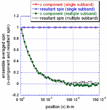
Figure 4: Spin relaxation in a $GaAs$ quantum wire of rectangular cross section $30$nm$\times 4$nm. The driving electric field is 2kV/cm and lattice temperature is $30$K. These results are obtained from Monte Carlo simulation described in [2], [3]. Spin does not relax for single channeled (single subband) transport, but does relax for multichanneled transport.

5 Conclusion

In this paper, we have established the origin of the D’yakonov-Perel’ spin relaxation in a quantum wire.This relaxation is harmful for most spintronic devices (one example is the SPINFET [1]), because it leads to spin randomization. Since optimum materials for SPINFET-type devices (e.g InAs) usually possess strong Rashba and also some Dresselhaus spin orbit interactions, the only effective way to eliminate the D’yakonov-Perel’ relaxation is to ensure and enforce single channeled transport. There has been recently some proposals that advocate using multi-channeled devices for SPINFET’s, along with the claim that they provide better spin control via the use of multiple gates [10]. While we do not believe that spin control is improved by using multiple gates since synchronizing these gates is an additional engineering burden that can only degrade device operation and gate control, it is even more important to understand that multi-channeled devices have serious drawbacks. The original proposal for the SPINFET pointed out that multi-channeled transport is harmful because it dilutes the spin interference effect which is the basis of the SPINFET device [1]. Here, we have pointed out an additional motivation to avoid multi-channeled devices: they will suffer from D’yakonov-Perel’ relaxation, while the single channeled device will not.

References

• [1] Datta, S. and Das, B., “Electronic analog of the electro-optic modulator”, Applied Physics Letters, (1990), 56, 665–667.
• [2] Pramanik, S., Bandyopadhyay, S. and Cahay, M., “Spin dephasing in quantum wires”, Physical Review B,(2003), 68, 075313-1 – 075313-10
• [3] Pramanik, S.,Bandyopadhyay, S. and Cahay, M., “Decay of spin-polarized hot carrier current in a quasi-one-dimensional spin-valve structure”, Applied Physics Letters, (2004), 84, 266–268.
• [4] Bychkov, Y. and Rashba, E., “Oscillatory effects and the magnetic susceptibility of carriers in inversion layers”, Journal of Physics C: Solid State Physics, (1984), 17, 6039–6045.
• [5] Dresselhaus, G., “Spin-orbit coupling effects in zinc blende structures”, Physical Review, (1955), 100, 580–586.
• [6] Saikin, S., Shen, M., Cheng, M. and Privman, V., “Semiclassical Monte Carlo model for in-plane transport of spin polarized electrons in III-V heterostructures”, Journal of Applied Physics, (2003), 94, 1769–1775.
• [7] Das, B., Datta, S. and Reifenberger, R., “Zero-field spin splitting in a two-dimensional electron gas”, Physical Review B, (1990), 41, 8278–8287.
• [8] Bournel, A., Dollfus, P., Bruno, P. and Hesto, P., “Spin polarized transport in 1D and 2D semiconductor heterostructures”, Materials Science Forum, (1999), 297–298, 205–212.
• [9] Bournel, A., Dollfus, P., Galdin, S., Musalem, F-X, and Hesto, P., “Modelling of gate induced spin precession in a striped channel high electron mobility transistor”, Solid State Communications, (1997), 104, 85–89.
• [10] Carlos Egues, J. and Burkard, G. and Loss, D., “Datta-Das transistor with enhanced spin control”, Applied Physics Letters, (2003), 82, 2658–2660.