Multiplicative versus additive noise in multi-state neural networks

Abstract

The effects of a variable amount of random dilution of the synaptic couplings in $Q$-Ising multi-state neural networks with Hebbian learning are examined. A fraction of the couplings is explicitly allowed to be anti-Hebbian. Random dilution represents the dying or pruning of synapses and, hence, a static disruption of the learning process which can be considered as a form of multiplicative noise in the learning rule. Both parallel and sequential updating of the neurons can be treated. Symmetric dilution in the statics of the network is studied using the mean-field theory approach of statistical mechanics. General dilution, including asymmetric pruning of the couplings, is examined using the generating functional (path integral) approach of disordered systems. It is shown that random dilution acts as additive gaussian noise in the Hebbian learning rule with a mean zero and a variance depending on the connectivity of the network and on the symmetry. Furthermore, a scaling factor appears that essentially measures the average amount of anti-Hebbian couplings.

Keywords: neural networks, multi-state neurons, stochastic dynamics, thermodynamics, dilution, additive noise, multiplicative noise.

1 Introduction

In general, artificial neural networks have been widely applied to memorize and retrieve information. During the last number of years there has been considerable interest in neural networks with multi-state neurons using the framework of statistical mechanics, which deals with large systems of stochastically interacting microscopic elements (see, e.g., [1] and references cited therein). In these models, the firing states of the neurons or their membrane potentials are the microscopic dynamical variables. Basically, compared to models with two-state (=binary) neurons, such models can function as associative memories for grey-toned or colored patterns [2, 3] and/or allow for a more complicated internal structure of the recall process, e.g., a distinction between the exact location and the details of a picture in pattern recognition and the analogous problem of retrieval focusing in the framework of cognitive neuroscience [4], a combination of information retrieval based on skills and based on specific facts or data [5, 6].

Different types of multi-state neurons can be distinguished according to the symmetry of the interactions between the different states. Here we are primarily interested in the so-called $Q$-Ising neuron, the states of which can be represented by scalars, and the interaction between two neurons can then be written as a function of the product of these scalars. So, the $Q$-states of the neuron can be ordered like a ladder between a minimum and a maximum value, usually taken to be $-1$ and $+1$. Special cases are $Q=2$, i.e., the well-known Hopfield model [7] and $Q=\infty$, i.e., networks with analogue or graded response neurons [8, 9, 10].

In analogy to the Hopfield model, the multi-state neuron models we discuss here have their immediate counterpart in random magnetic systems (=spin-glasses) (cfr., e.g., [11] and [12]), but with couplings defined in terms of embedded patterns through a learning rule. Since one of the aims of these networks is to find back the embedded patterns as attractors of the recall process, they are also interesting from the point of view of dynamical systems.

This close relation with spin-glass systems means that the methods and techniques used to study the latter have been successfully applied to these network models. In particular, it also means that concepts like temperature, fluctuations, disorder, noise, stochasticity …play a crucial role. In the literature it is well-known (see, e.g., [13]) that noise can have rather surprising and counterintuitive effects in the behavior of dynamical systems. It has been shown many times that noise can have a constructive rather than a destructive role. Relevant examples [13] of this fact are the phenomenon of stochastic resonance, noise induced ordering transitions, noise induced disordering phase transitions and an increase of the maximal information content with dilution in some neural network models [14]. In principle, these ordering effects seem to be related to the multiplicative character of the fluctuations, as compared to the disordering role of additive fluctuations. But things are not so simple because there is an interplay between additive and multiplicative noise terms.

Moreover, there are several types of internal fluctuations, e.g., thermal fluctuations introduced through a random term, quite often assumed to be gaussian distributed with zero mean and uncorrelated at different times. These internal fluctuations are described by an additive noise term, i.e., a random term that does not depend on the variable under consideration. This is not a necessary character of internal fluctuations. In some systems these can also be described by a multiplicative noise which is coupled to the state of the system. As a natural extension of the concept of internal fluctuations, external noise are those fluctuations that are not of thermal origin.

In the $Q$-Ising neural network models we are considering here, the following noise can be characterized. First, the neurons are stochastic such that the analogue of temperature is introduced. This enables us, as hinted at already above, to use the techniques of statistical mechanical mean-field theory, and ultimately to compute, e.g., the storage capacity of the network [1]. The zero-temperature limit will always reduce our system to a deterministic Hopfield or multi-state $Q$-Ising network. The meaning of this stochastic behavior is to model that neurons fire with variable strength, that there are delays in synapses, that there are random fluctuations in the release of transmitters …. Briefly, we model this internal noise by thermal fluctuations.

Secondly, in single pattern recall with many – a fraction of the size of the network – stored patterns there is the generally nontrivial interference noise due to the other patterns. This noise has been treated, e.g., by statistical neurodynamics [1, 15, 16] or functional integration methods [19, 17, 18, 14].

Thirdly, in the case of the Hopfield model the Hebb learning rule has been generalized in [20] in order to bring the model closer to natural systems. In particular, two types of noise terms have been added. The first one, an additive external contribution which is independent of the learning algorithm, and assumed to be gaussian distributed, is relaxing the hypothesis that the entire synaptic efficacy is coming from the learning process. The second one, a random multiplicative factor of order ${\cal O}(1)$, represents a static disruption of the learning process. An important example of the latter is random dilution of the network by the pruning or dying of synapses, relaxing the unrealistic condition that every neuron is connected to every other one. The effects of both these static fluctuations on the recall process in the Hopfield model have been estimated using equilibrium mean-field theory statistical mechanics. Technically speaking, the use of this method allows for symmetric dilution only, because the detailed balance principle, i.e., absence of microscopic probability currents in the stationary state, is needed to define an energy function. An additional remark is that non-linear updating of the synapses is allowed in that work. It has been shown that all these effects can be represented by an additive static gaussian noise in the learning rule and that the model is robust against the interference of this static noise.

In this contribution we extend the work of Sompolinsky [20] in different directions. Since we use both replica mean-field theory equilibrium methods and non-equilibrium functional integration techniques, the assumption of symmetric couplings is not required such that we can treat all forms of dilution. Moreover, we allow a fraction of the couplings to be anti-Hebbian [21]. We can also have sequential and parallel updating of the neurons, and we examine the effect of these noise terms in $Q$-Ising networks. The main results are that for the forms of dilution we have examined the effects can be represented by additive noise in the learning rule and a scaling factor proportional to the average amount of anti-Hebbian couplings. The diluted networks are robust under these effects.

The rest of this paper is organized as follows. In Section 2 we introduce the $Q$-Ising neural network model and the types of dilution we are interested in. Section 3 treats the statics of the model, where detailed balance requires, as we will explain, symmetric dilution. In Section 4 the dynamics of the network is studied allowing for a general form of dilution. Section 5 presents some concluding remarks.

2 $Q$-Ising networks with variable dilution

Consider a neural network consisting of $N$ neurons which can take values $\sigma_{i},i=1,\ldots,N$ from a discrete set ${\cal S}=\{-1=s_{1}<s_{2}<\ldots<s_{Q}=+1\}$. The $p$ patterns to be stored in this network are supposed to be a collection of independent and identically distributed random variables (i.i.d.r.v.), $\{{\xi}_{i}^{\mu}\in{\cal S}\}$, $\mu=1,\ldots,p$, with zero mean, $\left\langle\xi_{i}^{\mu}\right\rangle=0$, and variance $A=\left\langle(\xi_{i}^{\mu})^{2}\right\rangle$. The latter is a measure for the activity of the patterns. We remark that for simplicity we have taken these variables $s_{k},k=1,\ldots,Q$ equidistant and we have also taken the patterns and the neurons out of the same set of variables, but this is no essential restriction. Given the configuration ${\mbox{\boldmath$\sigma$}}_{N}(t)\equiv\{\sigma_{j}(t)\},j=1,\ldots,N$, the local field in neuron $i$ equals

$$h_{i}({\mbox{\boldmath$\sigma$}}_{N}(t))=\sum_{j=1}^{N}J_{ij}(t)\sigma_{j}(t)$$ (1)

with $J_{ij}$ the synaptic coupling from neuron $j$ to neuron $i$.

All neurons are updated sequentially or in parallel through the spin-flip dynamics defined by the transition probabilities

$$\Pr\{\sigma_{i}(t+1)=s_{k}\in{\cal S}|\mbox{\boldmath$\sigma$}_{N}(t)\}=\frac{\exp[-\beta\epsilon_{i}(s_{k}|\mbox{\boldmath$\sigma$}_{N}(t))]}{\sum_{s\in{\cal S}}\exp[-\beta\epsilon_{i}(s|\mbox{\boldmath$\sigma$}_{N}(t))]}\,.$$ (2)

The configuration ${\mbox{\boldmath$\sigma$}}_{N}(t=0)$ is chosen as input. Here the energy potential $\epsilon_{i}[s|{\mbox{\boldmath$\sigma$}}_{N}(t)]$ is defined by

$$\epsilon_{i}[s|{\mbox{\boldmath$\sigma$}}_{N}(t)]=-\frac{1}{2}[h_{i}({\mbox{\boldmath$\sigma$}}_{N}(t))s-bs^{2}]\,,$$ (3)

where $b>0$ is the gain parameter of the system. The zero temperature limit $T=\beta^{-1}\rightarrow 0$ of this dynamics is given by the updating rule

$$\sigma_{i}(t)\rightarrow\sigma_{i}(t+1)=s_{k}\qquad\mbox{such that}\qquad\min_{s\in{\cal S}}\epsilon_{i}[s|{\mbox{\boldmath$\sigma$}}_{N}(t)]=\epsilon_{i}[s_{k}|{\mbox{\boldmath$\sigma$}}_{N}(t)]\,.$$ (4)

This updating rule (4) is equivalent to using a gain function $\mbox{g}_{b}(\cdot)$,

$$\sigma_{i}(t+1) = \mbox{g}_{b}(h_{i}(\mbox{\boldmath$\sigma$}_{N}(t)))$$

$$\mbox{g}_{b}(x) \equiv \sum_{k=1}^{Q}s_{k}\left[\theta\left(b(s_{k+1}+s_{k})-x\right)-\theta\left(b(s_{k}+s_{k-1})-x\right)\right]$$ (5)

with $s_{0}\equiv-\infty$ and $s_{Q+1}\equiv+\infty$ and $\theta(\cdot)$ the Heaviside function. For finite $Q$, this gain function $\mbox{g}_{b}(\cdot)$ looks like a staircase with $Q$ steps. The gain parameter $b$ controls the average slope of $\mbox{g}_{b}(\cdot)$ and, hence, suppresses or enhances the role of the states around zero.

It is clear that the $J_{ij}$ explicitly depend on the architecture. We are interested in architectures with variable dilution and we also want to allow a fraction of the couplings to be anti-Hebbian. We realize this by choosing the couplings according to the Hebb rule multiplied with a factor $c_{ij}$

$$J_{ij}^{c}=\frac{c_{ij}}{c}J_{ij},\quad J_{ij}=\frac{1}{NA}\sum_{\mu=1}^{p}\xi_{i}^{\mu}\xi_{j}^{\mu}\quad\forall i,j\,,$$ (6)

with the $\{c_{ij}=0,\pm 1\},i,j=1,\ldots,N$ chosen to be i.i.d.r.v and obeying, in general, a distribution of the form

$$\textrm{P}[c_{ij}=x]=c_{1}\delta_{x,1}+c_{2}\delta_{x,-1}+(1-c_{1}-c_{2})\delta_{x,0}$$ (7)

with $c=c_{1}+c_{2}=\langle|c_{ij}|\rangle=\langle c_{ij}^{2}\rangle$ the connectivity, i.e., the average number of connections per neuron given by $cN$. In order to allow for variable symmetry as well, we define a joint-probability distribution for $i<j$ ($c_{ii}=1$)

$$\textrm{P}[(c_{ij},c_{ji})=(x,y)]= \quad\left(c_{1}^{2}+\frac{u+2v+w}{4}\right)\delta_{x,1}\delta_{y,1}+\left(c_{2}^{2}+\frac{u-2v+w}{4}\right)\delta_{x,-1}\delta_{y,-1}$$

$$+\left(c_{1}(1-c_{1}-c_{2})-\frac{v+w}{2}\right)\left(\delta_{x,1}\delta_{y,0}+\delta_{x,0}\delta_{y,1}\right)$$

$$+\left(c_{2}(1-c_{1}-c_{2})+\frac{v-w}{2}\right)\left(\delta_{x,0}\delta_{y,-1}+\delta_{x,-1}\delta_{y,0}\right)$$

$$+\left(c_{1}c_{2}-\frac{u-w}{4}\right)\left(\delta_{x,1}\delta_{y,-1}+\delta_{x,-1}\delta_{y,1}\right)$$

$$+\left((1-c_{1}-c_{2})^{2}+w\right)\delta_{x,0}\delta_{y,0}$$ (8)

with

$$u =\langle c_{ij}c_{ji}\rangle-\langle c_{ij}\rangle\langle c_{ji}\rangle=\langle c_{ij}c_{ji}\rangle-(c_{1}-c_{2})^{2}$$

$$v =\langle c_{ij}^{2}c_{ji}\rangle-\langle c_{ij}^{2}\rangle\langle c_{ji}\rangle=\langle c_{ij}^{2}c_{ji}\rangle-c(c_{1}-c_{2})$$

$$w =\langle c_{ij}^{2}c_{ji}^{2}\rangle-\langle c_{ij}^{2}\rangle\langle c_{ji}^{2}\rangle=\langle c_{ij}^{2}c_{ji}^{2}\rangle-c^{2}.$$ (9)

We note that these expressions are symmetric under the change $i\leftrightarrow j$.

These distributions generalize the following cases of random dilution frequently discussed in the literature (see, e.g., [1])

• Symmetric dilution where $c_{ij}=c_{ji}$ (SD): Due to the symmetry, $u=c-(c_{1}-c_{2})^{2}$, $v=(c_{1}-c_{2})(1-c_{1}-c_{2})$ and $w=c(1-c)$, yielding for eq. (2)

  $$\textrm{P}[(c_{ij},c_{ji})=(x,y)]=c_{1}\delta_{x,1}\delta_{y,1}+c_{2}\delta_{x,-1}\delta_{y,-1}+\left(1-c\right)\delta_{x,0}\delta_{y,0}$$ (10)

  whereby in most cases $c_{2}$ is taken to be zero, indicating that there are no anti-Hebbian couplings mixed in explicitly.

• Asymmetric dilution with $c_{ij}\neq c_{ji}$ and $c_{2}=0$ (AD): In this case $u=v=w=\langle c_{ji}c_{ji}\rangle-c^{2}$ and the joint-probability distribution eq. (2) becomes

  $$\textrm{P}[(c_{ij},c_{ji})=(x,y)]= (u+c^{2})\delta_{x,1}\delta_{y,1}+(c(1-c)-u)(\delta_{x,1}\delta_{y,0}+\delta_{x,0}\delta_{y,1})$$

  $$+(1+u-2c+c^{2})\delta_{x,0}\delta_{y,0}\,.$$ (11)

The meaning of the variable dilution as introduced in eq.(6)-(9) can best be understood from the theory of random graphs with $N$ nodes and $p$ the probability that any two of them are connected (see, e.g., [22]). The number of connections a node has for $N\rightarrow\infty$ (i.e., in the thermodynamic limit) goes to a Poisson distribution

$$P(n)=e^{\langle n\rangle}\frac{\langle n\rangle^{n}}{n!}$$ (12)

telling us that $\left\langle n\right\rangle=pN$ is the average number of connections per node. In order to indicate what range of dilution we allow for, we look at the diameter of the random graph, $d$, i.e., the maximum distance between any pair of nodes. This diameter is concentrated around

$$d=\frac{\log{(N)}}{\log{(\langle n\rangle)}}=\frac{\log{(N)}}{\log{(pN)}}\,.$$ (13)

The diameter is clearly 1 in the case that there is an edge with probability $1$ and, hence, we have a fully connected graph. The diameter diverges when $p\sim 1/N$. Given that $p$ scales with $N$ like $p\sim N^{z}$, several regimes containing different types of subgraphs can be distinguished as a function of $z$ [22]. In particular, it can be shown that the precise point above which the system becomes completely connected (such that it is always possible to find a path between any two nodes) is $\langle n\rangle\geq\log{(N)}$.

Looking at eq. (7) we find that this describes precisely a random graph with $c=c_{1}+c_{2}$ being the probability to have an edge. It follows that the average number of connections per neuron is $cN$. Since our $Q$-Ising network is taken to be a mean-field system characterized by an extensive number of long-range interactions we need to have that $\langle n\rangle=cN$ tends to infinity for $N\to\infty$ and all $c$. This implies that

$$\mbox{P}(|c_{ij}|=1)=\frac{\log{(N)}}{N}+c$$ (14)

such that $cN=\log{(N)}$ for $c=0$ and the complete connectivity of our model is still guaranteed. In this way, the diameter of our network is $d=1$ for $\forall c>0$ and $d=\infty$ when $c=0$, and the average number of connections is given by $\langle n\rangle=cN+\log{(N)}$. The limit $c\to 0$, i.e., the so-called extremely diluted limit has now a simple interpretation: each neuron has an infinite number of neighboring neurons but such that the average distance between any two neurons tends to infinity. All this is graphically illustrated in figure 1.

      

      

Figure 1: Effect of dilution. Top left: $c=1$ (fully connected); top right: $0<c<1$ (some couplings are cut); bottom left: $c=0$ (extreme dilution, tree-like structures); and bottom right: not all sites are connected (= finite connectivity).

We remark that in this way we can understand that eq. (6) has a well-defined meaning. There is a factor $cN$ in the denominator which always tends to infinity in the thermodynamic limit $N\to\infty$, whatever the value of $c$. Finally, we note that a distribution for the $c_{ij}$ can be chosen that does not support complete connectivity (see figure 1 bottom right), e.g., by taking $c=\tilde{c}/N$, with $\tilde{c}$ a fixed number independent of $N$. The system then consists of disjoint clusters of different sizes (=finite connectivity) [23]. These models are much more difficult to handle and are outside the scope of the present work.

3 Symmetric dilution and statics of the $Q$-Ising model

It is well-known that networks with symmetric couplings $J_{ij}$ obey the detailed balance principle. Systems with detailed balance can be described by standard equilibrium statistical mechanics making use of a Hamiltonian. The $Q$-Ising neural network we have defined in Section 2 is of a mean-field type with couplings (6) of infinite range and restricting ourselves to symmetric dilution $c_{ij}=c_{ji}$ (cfr., eq. (10)) the couplings $J_{ij}^{c}$ remain symmetric. The long time behavior of this network for sequential updating of the neurons is then governed by the following Hamiltonian

$$H=-\frac{1}{2}\sum_{i\neq j}J_{ij}^{c}\sigma_{i}\sigma_{j}+b\sum_{i}\sigma_{i}^{2}\,.$$ (15)

For parallel updating of the neurons a Hamiltonian is defined in terms of a two-spin representation [24] as

$$H=-\sum_{ij}J_{ij}^{c}\sigma_{i}\tau_{j}+b\sum_{i}(\sigma_{i}^{2}+\tau_{i}^{2})\,.$$ (16)

The thermodynamic properties of the system are then determined from the free energy using the standard techniques of replica mean-field theory [25, 26]. It is outside the scope of this contribution to go into the very details of these techniques but we indicate how the dilution is going to affect the calculations and the results.

The free energy is given as the logarithm of the partition function averaged over the disorder. This average is done using the replica technique such that we can write

$$Z^{n}({\mbox{\boldmath$\xi$}})=\underset{\mbox{\boldmath$\sigma$}}{\mbox{Tr}}\exp{\left(-\beta\sum_{\alpha=0}^{n}H({\mbox{\boldmath$\xi$}},{\mbox{\boldmath$\sigma$}}^{\alpha})\right)}$$ (17)

where $H({\mbox{\boldmath$\xi$}},{\mbox{\boldmath$\sigma$}}^{\alpha})$ is the Hamiltonian of each replica of the system given above and $\alpha$ is the replica index. Next, we first average this partition function over the dilution. At this point we remark that we consider the case of sequential updating. Parallel updating does not contain any additional difficulties [14]. Furthermore, we do not write explicitly the term proportional to $b$ in the Hamiltonian since it does not contain the $c_{ij}$ such that it can be inserted at any point of the calculation. Due to the central limit theorem we can easily see that $J_{ij}^{c}\sim\mathcal{O}((cN)^{-1/2})$, so that we can expand

$$Z^{n} =\underset{{\mbox{\boldmath$\sigma$}}}{\mbox{Tr}}\exp{\left(\frac{\beta}{2}\sum_{\alpha}\sum_{i,j\neq i}J_{ij}^{c}\sigma_{i}^{\alpha}\sigma_{j}^{\alpha}\right)}$$

$$=\underset{{\mbox{\boldmath$\sigma$}}}{\mbox{Tr}}\prod_{i<j}\left[1+\beta\sum_{\alpha}J_{ij}^{c}\sigma_{i}^{\alpha}\sigma_{j}^{\alpha}+\frac{\beta^{2}}{2}(J_{ij}^{c})^{2}\left(\sum_{\alpha}\sigma_{i}^{\alpha}\sigma_{j}^{\alpha}\right)^{2}+\mathcal{O}((cN)^{-3/2})\right]\,.$$ (18)

The average over the dilution variables $c_{ij}$ with $i<j$ denoted by $\left\langle\cdot\right\rangle_{\bf c}$ is then straightforward

$$\langle Z^{n}\rangle_{{\bf c}} =\underset{{\mbox{\boldmath$\sigma$}}}{\mbox{Tr}}\prod_{i<j}\left[1+\beta\,\,\frac{c_{1}-c_{2}}{c}\sum_{\alpha}J_{ij}\sigma_{i}^{\alpha}\sigma_{j}^{\alpha}+\frac{\beta^{2}}{2c}(J_{ij})^{2}\left(\sum_{\alpha}\sigma_{i}^{\alpha}\sigma_{j}^{\alpha}\right)^{2}+\mathcal{O}((cN)^{-3/2})\right]$$

$$\simeq\underset{{\mbox{\boldmath$\sigma$}}}{\mbox{Tr}}\exp{\left[\frac{\beta}{2}\,\,\frac{c_{1}-c_{2}}{c}\sum_{\alpha}\sum_{i,j\neq i}J_{ij}\sigma_{i}^{\alpha}\sigma_{j}^{\alpha}+\frac{\beta^{2}}{4}\,\,\frac{c-(c_{1}-c_{2})^{2}}{c^{2}}\sum_{i,j\neq i}(J_{ij})^{2}\left(\sum_{\alpha}\sigma_{i}^{\alpha}\sigma_{j}^{\alpha}\right)^{2}\right]}$$ (19)

where we have used that $J_{ij}\sim\mathcal{O}(N^{-1/2})$. Finally, noting that $(J_{ij})^{2}\rightarrow(\alpha c)/{N}+\mathcal{O}((cN)^{-2})$ as $N\rightarrow\infty$, with $\alpha={p}/(cN)$ the finite loading capacity, we write the replicated partition function averaged over the dilution as

$$\langle Z^{n}\rangle_{{\bf c}}=\underset{{\mbox{\boldmath$\sigma$}}}{\mbox{Tr}}\exp{\left[\frac{\beta}{2}\,\,\frac{c_{1}-c_{2}}{c}\sum_{\alpha}\sum_{i,j\neq i}J_{ij}\sigma_{i}^{\alpha}\sigma_{j}^{\alpha}+\frac{\beta^{2}\alpha}{4N}\,\,\frac{c-(c_{1}-c_{2})^{2}}{c}\sum_{i,j\neq i}\left(\sum_{\alpha}\sigma_{i}^{\alpha}\sigma_{j}^{\alpha}\right)^{2}\right]}\,.$$ (20)

Using a Hubbard-Stratonovich transformation this can be further expressed as

$$\langle Z^{n}\rangle_{{\bf c}}=\left\langle\underset{{\mbox{\boldmath$\sigma$}}}{\mbox{Tr}}\exp{\left[\frac{\beta}{2}\sum_{\alpha}\sum_{i,j\neq i}\left(\frac{c_{1}-c_{2}}{c}J_{ij}+d_{ij}\right)\sigma_{i}^{\alpha}\sigma_{j}^{\alpha}\right]}\right\rangle_{{\bf d}}$$ (21)

with $\left\langle\cdot\right\rangle_{\bf d}$ indicating the average over the $d_{ij}$, a set of i.i.d.r.v. for $i<j$ and symmetric with $d_{ii}=0$. They obey a gaussian distribution with mean $\langle d_{ij}\rangle=0$ and variance $\langle d_{ij}^{2}\rangle=\alpha s/(cN)$ with $s=c-(c_{1}-c_{2})^{2}$. This shows that the symmetric dilution (10), being a form of multiplicative noise, introduces an effective Hamiltonian where the learning rule now contains an additive noise term plus a scaling of the Hebbian part

$$J_{ij}^{c}=J_{ij}\frac{c_{ij}}{c}\quad\rightarrow\quad J_{ij}^{c}=\frac{c_{1}-c_{2}}{c}J_{ij}+d_{ij}\,.$$ (22)

The scaling factor expresses the influence of explicitly allowing an average amount $c_{2}=\textrm{P}[c_{ij}=-1]$ of anti-Hebbian couplings. For $c_{2}=0$ the scaling term is $1$ and in this case the expression (22) agrees with the results of Sompolinsky [20] for the Hopfield model $Q=2$ and with the results of Theumann and Erichsen [27] for the symmetrically diluted $Q$-Ising model.

An analogous calculation can be performed for parallel updating of the neurons leading precisely to eq. (21) with $\sigma_{j}^{\alpha}$ replaced by $\tau_{j}^{\alpha}$ and with the factor $1/2$ removed. In all these calculations we have only used the first and second moments of the probability distribution for the $c_{ij}$. This is due to the mean-field character of the network we have treated. Therefore, one can easily extend this result to any (symmetric) multiplicative noise such that

$$J_{ij}^{m}=J_{ij}\frac{\eta_{ij}}{\eta}\quad\rightarrow\quad J_{ij}^{a}=\frac{\sqrt{\eta-s}}{\eta}J_{ij}+\sqrt{\frac{\alpha s}{\eta N}}d^{\prime}_{ij},$$ (23)

with obvious meaning of the superscripts $m$ and $a$, with $d^{\prime}_{ij}=\mathcal{N}(0,1)$ a gaussian with mean zero and variance $1$, and with $\eta=\langle\eta_{ij}^{2}\rangle$ and $s=\eta-\langle\eta_{ij}\rangle^{2}$ characterizing the multiplicative noise.

To close this Section we remark that when we are interested in the further calculation of the free energy, e.g., in order to obtain the equilibrium fixed-point equations and the loading capacity we have to average the partition function (21) over the pattern distribution employing the standard techniques. We refer to the literature for the final results [27, 14].

4 General dilution and dynamics of the $Q$-Ising model

For asymmetric dilution (recall, e.g., (• ‣ 2)) the system we have defined does not obey detailed balance. In this case we have to resort to techniques used in non-equilibrium statistical mechanics. The method we use to study the effect of general dilution in the dynamics is the generating functional approach [19, 18].

The idea of this approach is to look at the probability to find a certain microscopic path in time. The basic tool to study the statistics of these paths is the generating function

$$\big{\langle}\big{\langle}Z[{\bf\Phi}]\big{\rangle}_{{\bf c}}\big{\rangle}_{{\mbox{\boldmath$\xi$}}}=\sum_{{\mbox{\boldmath$\sigma$}}(0)}...\sum_{{\mbox{\boldmath$\sigma$}}(t)}\exp{\left(-i\sum_{s=0}^{t}\sum_{i=1}^{N}(\phi_{i}(s)\sigma_{i}(s))\right)}\big{\langle}\big{\langle}\mbox{P}[{\mbox{\boldmath$\sigma$}}(0)...{\mbox{\boldmath$\sigma$}}(t)]\big{\rangle}_{{\bf c}}\big{\rangle}_{{\mbox{\boldmath$\xi$}}}$$ (24)

where the dilution and pattern averages are denoted by $\big{\langle}\big{\langle}\cdot\big{\rangle}_{{\bf c}}\big{\rangle}_{{\mbox{\boldmath$\xi$}}}$ and where $\mbox{P}[{\mbox{\boldmath$\sigma$}}(0)...{\mbox{\boldmath$\sigma$}}(t)]$ is the probability to have a certain path in phase space

$$\mbox{P}[{\mbox{\boldmath$\sigma$}}(0)...{\mbox{\boldmath$\sigma$}}(t)]=\mbox{P}[{\mbox{\boldmath$\sigma$}}(0)]\prod_{t^{\prime}=0}^{t-1}W[{\mbox{\boldmath$\sigma$}}(t^{\prime})|{\mbox{\boldmath$\sigma$}}(t^{\prime}-1)]$$ (25)

with $W[{\mbox{\boldmath$\sigma$}}(t^{\prime})|{\mbox{\boldmath$\sigma$}}(t^{\prime}-1)]$ the transition probabilities from ${\mbox{\boldmath$\sigma$}}(t^{\prime}-1)$ to ${\mbox{\boldmath$\sigma$}}(t^{\prime})$. For the $Q$-Ising network with parallel updating they read

$$W[{\mbox{\boldmath$\sigma$}}(t^{\prime})|{\mbox{\boldmath$\sigma$}}(t^{\prime}-1)]=\prod_{i=1}^{N}\frac{\exp{\left(\beta\sigma_{i}(t^{\prime})\sum_{j}J_{ij}^{c}\sigma_{j}(t^{\prime}-1)-\beta b\sigma_{i}^{2}(t^{\prime})\right)}}{\underset{\sigma}{\textrm{Tr}}\exp{\left(\beta\sigma\sum_{j}J_{ij}^{c}\sigma_{j}(t^{\prime}-1)-\beta b\sigma^{2}\right)}}\,.$$ (26)

We remark again that sequential updating can be treated in an analogous way. Furthermore, we note that one can obtain all the order parameters of the system through derivation of the generating function, e.g., the overlap between the network configuration and an embedded pattern is given by

$$m(t)=\frac{1}{A}\big{\langle}\big{\langle}\xi_{i}\sigma_{i}(t)\big{\rangle}_{{\bf c}}\big{\rangle}_{{\mbox{\boldmath$\xi$}}}=i\,\lim_{{\bf\Phi}\rightarrow 0}\frac{1}{A}\Big{\langle}\Big{\langle}\frac{\xi_{i}\,\partial Z[{\bf\Phi}]}{\partial\phi_{i}(t)}\Big{\rangle}_{{\bf c}}\Big{\rangle}_{{\mbox{\boldmath$\xi$}}}\,.$$ (27)

Introducing the local fields ${\bf h}=\{h_{i}(s)=\sum_{j}J_{ij}^{c}\sigma_{j}(s)\}$ and their conjugates $\hat{\bf h}$, we arrive at

$$\big{\langle}\big{\langle}Z[{\bf\Phi}]\big{\rangle}_{{\bf c}}\big{\rangle}_{{\mbox{\boldmath$\xi$}}} =\int\{d{\bf h}\}\{d\hat{{\bf h}}\}\sum_{{\mbox{\boldmath$\sigma$}}(0)}...\sum_{{\mbox{\boldmath$\sigma$}}(t)}\mbox{P}[{\mbox{\boldmath$\sigma$}}(0)]\prod_{s>0}^{t}\prod_{i}\mbox{P}[\sigma_{i}(s)|h_{i}(s-1),b]$$

$$=\exp{\left(N\mathcal{F}[{\mbox{\boldmath$\sigma$}},\hat{{\bf h}}]\right)}\prod_{i}\prod_{s=0}^{t}\exp{\left(i\hat{h}_{i}(s)h_{i}(s)-i\phi_{i}(s)\sigma_{i}(s)\right)}$$ (28)

where the disorder and dilution are put in one term

$$\mathcal{F}[{\mbox{\boldmath$\sigma$}},\hat{{\bf h}}]=\frac{1}{N}\log{\left(\Bigg{\langle}\Bigg{\langle}\exp{\left[-i\sum_{i}\sum_{s=0}^{t}\hat{h}_{i}(s)\sum_{j}J_{ij}^{c}\sigma_{j}(s)\right]}\Bigg{\rangle}_{{\bf c}}\Bigg{\rangle}_{{\mbox{\boldmath$\xi$}}}\right)}\,.$$ (29)

We do not report the whole treatment of the generating function here but refer to, e.g., [19] for more details on the method. We do discuss in detail, however, the dilution average since this is precisely the subject of our study.

As in the statics we use that the diluted couplings $J_{ij}^{c}$ are of order $\mathcal{O}((cN)^{-1/2})$ and that the $J_{ij}\sim\mathcal{O}(N^{-1/2})$. We note that, in principle, diagonal coupling terms usually taken to be of the form $J_{ii}=\alpha J_{0}$ can be present, but they are taken out separately because they do not need to be averaged over. Introducing then $b_{ij}=\sum_{s}\hat{h}_{i}(s)\sigma_{j}(s)$ and using the fact that the distribution for the asymmetric dilution eq. (2) is i.i.d.r.v. for $i<j$ we can write

$$\bigg{\langle}\cdot\bigg{\rangle}_{{\bf c}} =\prod_{i<j}\big{\langle}\exp{[-i(J_{ij}^{c}b_{ij}+J_{ji}^{c}b_{ji})]}\Big{\rangle}_{(c_{ij},c_{ji})}$$

$$=\prod_{i<j}\Big{\langle}1-\frac{i}{c}J_{ij}\left(c_{ij}b_{ij}+c_{ji}b_{ji}\right)-\frac{1}{2c^{2}}J_{ij}^{2}\left(c_{ij}b_{ij}+c_{ji}b_{ji}\right)^{2}+\mathcal{O}((cN)^{-3/2})\Big{\rangle}_{(c_{ij},c_{ji})}$$

$$=\prod_{i,j\neq i}\exp{\left[-i\,\,\frac{c_{1}-c_{2}}{c}J_{ij}b_{ij}-\frac{s}{4c^{2}}J_{ij}^{2}(b_{ij}+b_{ji})^{2}-\frac{u-s}{2c^{2}}J_{ij}^{2}b_{ij}b_{ji}\right]}$$

$$=\prod_{i,j\neq i}\exp{\left[-i\,\,\frac{\sqrt{c-s}}{c}J_{ij}b_{ij}-\frac{s}{2c^{2}}J_{ij}^{2}(w_{+}b_{ij}+w_{-}b_{ji})^{2}\right]}$$ (30)

where we have introduced a number of shorthand notations

$$s=c-(c_{1}-c_{2})^{2}\,,\qquad w_{\pm}=\sqrt{\frac{1\pm\sqrt{1-\Gamma^{2}}}{2}}\,,\qquad\Gamma\equiv\frac{u}{s}=\frac{\langle c_{ij}c_{ji}\rangle-\langle c_{ij}\rangle^{2}}{\langle c_{ij}^{2}\rangle-\langle c_{ij}\rangle^{2}}=\frac{\langle c_{ij}c_{ji}\rangle-(c_{1}-c_{2})^{2}}{c-(c_{1}-c_{2})^{2}}\,.$$ (31)

We remark that the parameter $\Gamma$ is a measure for the symmetry in the $c_{ij}$, and takes values in the range $[-1,1]$; $\Gamma=1$ is complete symmetry, $\Gamma=-1$ is complete antisymmetry. Finally, a Hubbard-Stratonovich transformation can be done as before leading to

$$\bigg{\langle}\cdot\bigg{\rangle}_{{\bf c}}=\Bigg{\langle}\prod_{i,j\neq i}\exp{\left[-i(\frac{c_{1}-c_{2}}{c}J_{ij}+[w_{+}d_{ij}+w_{-}d_{ji}])b_{ij}\right]}\Bigg{\rangle}_{{\bf d}}$$ (32)

where the $d_{ij}$ are a set of i.i.d.r.v. for $i<j$, symmetric, $d_{ij}=d_{ji}$, and obeying a gaussian probability distribution with $\langle d_{ij}\rangle=0$ and $\langle d_{ij}^{2}\rangle=sJ_{ij}^{2}/c^{2}$. This shows that also general asymmetric dilution can be written as additive noise in the learning rule with a scaling of the Hebbian part

$$J_{ij}^{c}=J_{ij}\frac{c_{ij}}{c}\quad\rightarrow\quad J_{ij}^{c}=\frac{\sqrt{c-s}}{c}J_{ij}+\sqrt{\frac{\alpha s}{cN}}(w_{+}d^{\prime}_{ij}+w_{-}d^{\prime}_{ji}),$$ (33)

where now $d^{\prime}_{ij}=\mathcal{N}(0,1)$. We note explicitly that the parameters $v$ and $w$ (recall eq. (9)) do not play a role in the calculation. Only the mean $c$, the variance $s$ and the covariance $u$ of the probability distribution for the random dilution are important. Again, for $c_{2}=0$ the scaling factor expressing the explicit mixing in of anti-Hebbian couplings is $1$ and in the symmetric case (SD), $\Gamma=1$ in addition, such that the additive noise reduces to $J_{ij}^{c}=J_{ij}+d_{ij}$ (see eq. (22)).

As in the statics, the calculation of the dynamics can be pursued by doing the average over the patterns and expressions for the overlap, correlation functions and response functions can be obtained. This is beyond the purpose of the present contribution and will be presented in [14]. Finally, the remarks made before that sequential dynamics can be treated similarly and that the effective dynamics is formally the same, boil down to the fact that the explicit form of the transition rates is not needed to derive the effective path average. Only the initial conditions need to factorize over the site index $i$ and this is a characteristic property of mean-field systems.

Using the generating functional approach it is clear that the effect of random dilution on the learning rule in neural networks based on other types of multi-state neurons [1], e.g., Blume-Emery-Griffiths neurons, Potts neurons, Ashkin-Teller neurons can be examined in an analogous way.

5 Concluding remarks

In this work we have examined the effects of general random dilution, which can be considered as a static disruption of the learning process and, hence, as a form of multiplicative noise in the Hebbian learning rule, on the statics and dynamics of $Q$-Ising multi-state neural networks. A fraction of the couplings is explicitly taken to be anti-Hebbian. Both sequential updating and parallel updating of the neurons are allowed.

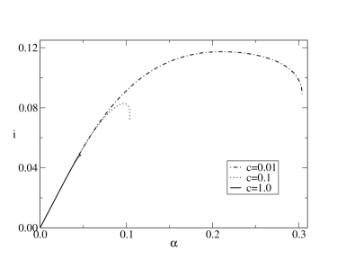
Figure 2: Information content $i$ as a function of the loading capacity $\alpha$ for the $Q=3$ Ising model with uniform patterns ($A=2/3$), $b=0.5$, $T=0$, and symmetric dilution with $c_{2}=0$ and $c_{1}=c=0.01$, $0.1$ and $1.0$.

It is shown, using replica mean-field theory, that for symmetric dilution the effect on the learning rule appears as additive gaussian noise together with a scaling of the Hebbian part. This scaling is a measure for the average amount of anti-Hebbian couplings and becomes $1$ when no such couplings are present. This extends previous results in the literature. Moreover, for general dilution, including asymmetric forms, a similar result is obtained using the generating functional approach employed in studies of the dynamics of disordered systems. The additive noise is determined as a function of the mean, the variance and the covariance of the probability distribution characterizing the dilution. We conjecture that this result is valid for any network of mean-field type.

Although this is beyond the scope of the present work it is relevant to remark that it can be shown that the type of multi-state networks studied here are robust against the interference of static noise coming from random dilution (cfr., e.g., [14, 20]) in the sense that the quality of the retrieval properties is affected very little, unless the amount of dilution is very high. As an illustration of this fact we show in fig. 2 the information content, being the product of the loading capacity and the mutual information, of a $Q=3$-Ising neural network with parameters as indicated in the figure caption for several amounts of symmetric dilution $c$. For more details on this we refer to [14].

The fact that the effect of random dilution can be expressed as additive noise in the learning rule makes the analytical calculations on these networks easier and more transparent and can be of help in the non-trivial numerical simulations of diluted systems.

6 Acknowledgements

We thank Rubem Erichsen Jr. for informative discussions. This work has been supported in part by the Fund of Scientific Research, Flanders-Belgium.

References

- [1] D. Bollé, “Multi-state neural networks based upon spin-glasses: a biased overview”, in Advances in Condensed matter and statistical Mechanics, eds. S. Korutcheva and R. Cuerno, (Commack, NY: Nova Science Publishers), to appear, 2004
- [2] T. Tadaki and J. Inoue, “Multi-state image restoration by transmission of bit-composed data”, Phys. Rev. E 65, 016101, 2001
- [3] J. Inoue and D.M. Carlucci, “Image restoration using the -Ising spin-glass”, Phys. Rev. E 64, 036121, 2001.
- [4] D.L. Schacter, K.A. Norman and W. Koutstaal, “The cognitive neuroscience of constructive memory”, Annu. Rev. Psychol. 49, 289, 1998
- [5] H. Komatsu and Y. Ideura, “Relationship between color, shape and pattern selectivity of neurons in the inferior temporal cortex of the monkey”, J. Neurophysiol. 70, 677, 1993
- [6] L.R. Squire, “Mechanisms of memory”, Science 232, 1612, 1986
- [7] J.J. Hopfield, “Neural networks and physical systems with emergent collective computational abilities”, Proc. Nat. Acad. Sci. USA 79, 2554, 1982
- [8] J.J. Hopfield, “Neurons with graded response have collective computational properties like those of two-state neurons”, Proc. Nat. Acad. Sci. USA 81, 3088, 1984
- [9] C.M. Marcus and R.M. Westerfelt, “Dynamics of iterated-map networks”, Phys. Rev. A 40, 501, 1989
- [10] C.M. Marcus, F.M. Waugh and R.M. Westerfelt, “Associative memory in an analog iterated-map neural network”, Phys. Rev. A 41, 3355, 1990
- [11] D. Sherrington and S. Kirkpatrick, “ Solvable model of a spin-glass”, Phys. Rev. Lett. 35, 1792, 1972
- [12] S.K. Ghatak and D. Sherrington, “Crystal field effects in a general S-Ising spin-glass”, J. Phys. C: Solid State Physics 10, 3149, 1977
- [13] J. García-Ojalvo and J.M. Sancho, Noise in Spatially Extended Systems, Springer, NY, 1999
- [14] D. Bollé, R. Erichsen Jr and T. Verbeiren, “Parallel versus sequential dynamics of -Ising neural networks”, in preparation
- [15] S. Amari and K. Maginu, “Statistical neurodynamics of associative memory”, Neural Networks 1, 63, 1988
- [16] H. Nishimori, Statistical Physics of Spin Glasses and Information Processing, Oxford Univ. Press, 2001
- [17] E.D. Siggia, P.C. Martin and H.A. Rose, “Statistical dynamics of classical systems”, Phys. Rev. A 8, 423, 1973
- [18] C. De Dominicis, “Dynamics as a substitute for replicas in systems with quenched random impurities” J. Phys. A: Math. Gen. 18, 4913, 1978
- [19] A.C.C. Coolen, “Statistical Mechanics of Recurrent Neural Networks II-Dynamics”, in Handbook of Biological Physics Vol 4, ed. by F. Moss and S. Gielen, Elsevier Science, 597, 2001
- [20] H. Sompolinsky, “Neural networks with nonlinear synapses and a static noise”, Phys. Rev. A 34, 2571, 1986
- [21] J.J. Hopfield, D.I. Feinstein and R.G. Palmer, “Unlearning has a stabilizing effect in collective memories”, Nature 304, 158, 1983
- [22] B. Bollobàs, Modern Graph Theory, Springer, New York, 1998
- [23] B. Wemmenhove and A.C.C. Coolen, “Finite connectivity attractor neural networks”, J. Phys. A: Math. Gen., 36, 9617, 2003.
- [24] P. Peretto, “Collective properties of a neural network: a statistical physics approach”, Biol. Cybern., 50, 51, 1984
- [25] L. Viana and A.J. Bray, “Phase diagrams for dilute spin glasses”, J. Phys. C: Solid State Physics, 18, 3037, 1985
- [26] M. Mézard, G. Parisi and M.A. Virasoro, Spin glass theory and beyond, World Scientific, Singapore, 1987
- [27] W.K. Theumann and R. Erichsen Jr., “Retrieval behavior and thermodynamic properties of symmetrically diluted -Ising neural networks”, Phys. Rev. E 64, 061902, 2001