A Simulation Method to Resolve Hydrodynamic Interactions in Colloidal Dispersions

Abstract

A new computational method is presented to resolve hydrodynamic interactions acting on solid particles immersed in incompressible host fluids. In this method, boundaries between solid particles and host fluids are replaced with a continuous interface by assuming a smoothed profile. This enabled us to calculate hydrodynamic interactions both efficiently and accurately, without neglecting many-body interactions. The validity of the method was tested by calculating the drag force acting on a single cylindrical rod moving in an incompressible Newtonian fluid. This method was then applied in order to simulate sedimentation process of colloidal dispersions.

I Introduction

There are a number of useful systems consisting of small solid particles dispersed in host fluids. Among them, colloidal dispersions are most common to our daily life and are of great importance, particularly in the fields of engineering and biology Russel et al. (1989); Larson (1999). Colloidal dispersions have been reported to exhibit several unusual phenomena, such as long-range correlations in sedimenting particles Segré et al. (2001), long-range anisotropic interactions in liquid crystal colloidal dispersions Stark (2001), transient gel formations during phase separations of colloidal suspensions Tanaka (1999), and electro-rheological effects in particle suspensions of nonconductive fluids Winslow (1949).

Since the dynamics of colloidal dispersions are very complicated, it is extremely difficult to investigate their dynamic properties by means of analytical methods alone. Computational approaches are necessary in order to elucidate the true mechanisms of dynamic phenomena in a variety of situations. Colloidal dispersions, however, have a typical multi-scale problem. The molecules comprising host fluids are much smaller and move much faster than colloidal particles. From a computational point of view, performing fully microscopic molecular simulations for this kind of multi-scale system is extremely inefficient. An alternative, which is generally considered much better than microscopic simulations, is to treat host fluids as coarse-grained continuum media.

Several numerical methods have been developed in an effort to simulate colloidal dispersions. Two of the most well known methods are the Stokesian dynamics Brady and Bossis (1988) and the Eulerian–Lagrangian method. The former is thought to be the most efficient Method, capable of treating hydrodynamic interactions properly. Furthermore, it can be implemented as $O(N_{p})$ scheme for $N_{p}$ particles by utilizing the fast multipole method Ichiki (2002). However, it is extremely difficult to deal with dense dispersions and dispersions consisting of non-spherical particles by means of Stokesian dynamics due to the complicated mathematical structures used in Stokesian dynamics. On the other hand, the Eulerian–Lagrangian method is a very natural and sensible approach to simulate solid particles with arbitrary shapes. A number of kinds of tailor-made mesh, including unstructured mesh, overset mesh, and boundary-fitted coordinates, have been applied to specific problems, so that the shapes of the particles are properly expressed in the discrete mesh-space. Thus, in principle it is possible to apply this method to dispersions consisting of many particles with any shape. However, a numerical inefficiency arises from the following: i) re-constructions of the irregular mesh are necessary at every simulation step according to the temporal particle position, and ii) the Navier–Stokes equation must be solved with boundary conditions imposed on the surfaces of all colloidal particles. The computational demands thus are enormous for systems involving many particles, even if the shapes are all spherical.

Thus, our goal is to develop an efficient simulation method that can be applied to particle dispersions in complex fluids. Since host fluids are considered incompressible in such systems, an efficient simulation must address how to efficiently and accurately evaluate hydrodynamic interactions. As a first step towards this goal, we attempted to develop a method to simulate colloidal dispersions in simple Newtonian fluids. The reliability of this method was tested by calculating the drag force acting on a cylindrical object in a flow. Its performance was subsequently demonstrated by simulating the sedimentation processes of colloidal particles in a Newtonian fluid within a small Reynolds number regime.

II Simulation method

In order to overcome the problems arising at the solid-fluid interface in the Eulerian–Lagrangian method, rather than the original discontinuous rectangle profile (interfacial thickness, $\xi=0$) schematically depicted in Fig. 1, a smoothed profile was introduced to the interface ($\xi>0$). This simple modification greatly benefits the performance of numerical computations, compared to the original Eulerian–Lagrangian method for the following reasons.

Figure 1: An example of the smoothed profile (dashed line). The original rectangular profile is also shown for comparison (solid line).

i) Regular Cartesian coordinates can be used for many particle systems with any particle shape, rather than boundary-fitted coordinates. The solid-fluid interface has a finite volume ($\propto\pi a^{d-1}\xi$, with $a$ and $d$ as the particle radius and system dimension) supported by multiple grid points. Thus, the round particle shape can be treated in fixed Cartesian coordinates without difficulty. The simulation scheme is thus free from the mesh re-construction problem that significantly suppresses the computational efficiency of the Eulerian–Lagrangian method. In addition, the simple Cartesian coordinate enables use of the periodic boundary conditions as well as the fast Fourier transformation (FFT).

ii) At the interfaces, the velocity component in the direction normal to the interface of the host fluid must be equal to that of the particle. This kinetic condition is imposed in the Navier–Stokes equation, as the boundary value condition defined for the solid-fluid interface in typical methods. In our method, however, this condition is automatically satisfied by an incompressibility condition on the entire domain, which will be subsequently explained in detail.

iii) The computational demands for this method include sensitivity to the number of grid points (volume of the total system), however it is insensitive to the number of particles. Thus, our method is thought to be suitable for simulating dense colloidal dispersions.

The non-zero interfacial thickness $\xi$ is the only approximation used in the present method. Thus, inter-particle hydrodynamic interactions can be fully resolved within the approximation of the non-zero thickness in the present method.

There have been two similar methods developed by different authors Glowinski et al. (2001); Höfler and Schwarzer (2000). The basic ideas of these methods is to use a fixed grid and represent the particles not as boundary conditions to the fluid, but by a body force or Lagrange multipliers in Navier–Stokes equation. The essential difference in our approach to these two methods is to introduce a explicit diffuse interface in a smoothed profile. As long as a fixed grid is used, the moving boundary is inevitably represented as diffuse as grid spacing. The introduction of a explicit smoothed profile makes us to present a clear formulation of a numerical algorithm and is advantagous when it is applied to complex fluids Yamamoto (2001); Yamamoto et al. (2004)

The lattice Boltzmann (LB) method Succi (2001) has attracted much attention in recent years to simulate colloidal dispersions with hydrodynamic interactions Ladd and Verberg (2001). The LB equation was proved to offer a faithful discretization of Navier–Stokes equation, and colloidal dispersions are simulated in the Eulerian–Lagrangian manner. In practical viewpoints, the LB method is forumlated on a fixed Cartesian lattice and is well adapted to parallel computation. The LB approach, although the formulation is not intuitive and its treatment of moving solid-fluid boundary is somewhat complicated, has several similar merits to the present method.

The “fluid particle dynamics” (FPD) method was proposed earlier and is similar to our method in spirit Tanaka and Araki (2000). In this method, although a similar smoothed profile was adopted, there are several important differences between FPD and the present method. The most significant difference is that particles are modeled as a highly viscous fluid with viscosity $\eta_{c}$, much greater than the fluid viscosity $\eta_{s}$ in FPD. This enables the rigidity of the particles to be sustained approximately by artificial diffusivity $\Delta\eta\phi(\mbox{\boldmath$x$},t)$ ($\Delta\eta\equiv\eta_{c}-\eta_{s}\gg\eta_{s}$) within the particle domain. While this model is physically correct, a practical problem remains in that a larger viscosity requires smaller time increments. In contrast, the present method treats colloidal particles as undeformable solids, (i.e., $\Delta\eta\to\infty$) thus no additional constraint arises in the numerical implementations.

II.1 Basic working equations

Colloidal dispersions are considered in a simple Newtonian liquid. The motion of the host fluid is governed by the Navier–Stokes equation with the incompressibility condition,

$$\left(\partial_{t}+\mbox{\boldmath$u$}_{f}\cdot\nabla\right){\mbox{\boldmath$u$}_{f}} = \frac{1}{\rho}\nabla\cdot\mbox{\boldmath$\sigma$}_{f},$$ (1)

$$\nabla\cdot\mbox{\boldmath$u$}_{f} = 0$$ (2)

where $\mbox{\boldmath$u$}_{f}$ is the fluid velocity, $\rho$ is the fluid density. The stress tensor is represented by,

$$\mbox{\boldmath$\sigma$}_{f} = -p\mbox{\boldmath$I$}+\eta\left\{\nabla\mbox{\boldmath$u$}_{f}+\left(\nabla\mbox{\boldmath$u$}_{f}\right)^{T}\right\}$$ (3)

where $p$ is the pressure, $\eta$ is the fluid viscosity.

The colloidal particles are assumed to be rigid and spherical, and their positions $\mbox{\boldmath$R$}_{i}$ are tracked in a Lagrangian reference frame,

$$\dot{\mbox{\boldmath$R$}_{i}} = \mbox{\boldmath$V_{i}$},$$ (4)

with the translational momentum equation

$$M_{i}\dot{\mbox{\boldmath$V$}_{i}} = \mbox{\boldmath$F$}^{H}_{i}+\mbox{\boldmath$F$}^{PP}_{i}+\mbox{\boldmath$F$}^{g}_{i},$$ (5)

and the angler momentum equation

$$\mbox{\boldmath$I$}_{i}\cdot\dot{\mbox{\boldmath$\Omega$}}_{i} = \mbox{\boldmath$N$}^{H}_{i},$$ (6)

where $\mbox{\boldmath$R$}_{i}$, $\mbox{\boldmath$V$}_{i}$, $\mbox{\boldmath$\Omega$}_{i}$, $M_{i}$, and $\mbox{\boldmath$I$}_{i}$ are the position, the translational velocity, the angular velocity, the mass, and the inertia tensor of the $i$th particle, respectively. The hydrodynamic force $\mbox{\boldmath$F$}_{i}^{H}$ and torque $\mbox{\boldmath$N$}_{i}^{H}$ acting on a particle can be obtained by integrating the stress tensor over the surface as

$$\mbox{\boldmath$F$}^{H}_{i} = \int_{S_{i}}\mbox{\boldmath$\sigma$}_{f}\cdot d\mbox{\boldmath$S$}$$ (7)

$$\mbox{\boldmath$N$}^{H}_{i} = \int_{S_{i}}\mbox{\boldmath$r$}\times\left(\mbox{\boldmath$\sigma$}_{f}\cdot d\mbox{\boldmath$S$}\right),$$ (8)

where $r$ is the relative position vector from the center of rotation to the colloid surface. Furthermore, $\mbox{\boldmath$F$}^{PP}_{i}$ is the force due to direct particle-particle interactions, and $\mbox{\boldmath$F$}^{g}_{i}=M_{i}(1-\rho_{*}^{-1})\mbox{\boldmath$g$}$ is the buoyant force where $\rho_{*}=\rho_{c}/\rho$ is the mass density ratio of the particles to the host fluid, and $g$ is the gravitational acceleration. Relevant dimensionless parameters in the above equations include the Reynolds number $Re=UL/\nu$, the Froude number $Fr=U/\sqrt{gL}$, the mass density ratio $\rho_{*}$, and the volume fraction $\alpha$. Here $U$ and $L$ represent typical velocity and length scales specific to the systems under consideration, respectively. The kinematic viscosity $\nu=\eta/\rho$ and the mass density of colloidal particles $\rho_{c}$ are assumed to be constant.

In typical methods, the above set of equations should be solved using proper boundary conditions defined at the solid-fluid interface. In the present method, however, the solid-fluid boundary condition is replaced with a body force and an incompressibility condition on a total velocity defined on the entire domain.

II.2 Modified working equations

Assuming a smoothed profile with a finite thickness $\xi$ to the solid-fluid interface, we here derive the body force which accurately takes the interactions between solids and fluids due to the motions of colloids in an incompressible fluid into consideration. The present study considers a mono-disperse system consisting of $N$ spherical particles with radius $a$. The positions of the particles $\{\mbox{\boldmath$R$}_{1},\cdots,\mbox{\boldmath$R$}_{N}\}$ are first transformed to a continuous field

$$\phi(\mbox{\boldmath$x$},t) \equiv \sum_{i=1}^{N}\phi_{i}(\mbox{\boldmath$x$},t),$$ (9)

using the $i$th particle’s profile function $\phi_{i}(\mbox{\boldmath$x$})$ centered at $\mbox{\boldmath$R$}_{i}$. Several possible mathematical forms for $\phi_{i}(\mbox{\boldmath$x$})$ exist, however, some typical functions are listed in Appendix A.

The continuum velocity field $\mbox{\boldmath$u$}_{p}$ is defined for the solid particles using $\{\mbox{\boldmath$V$}_{1},\cdots,\mbox{\boldmath$V$}_{N}\}$, $\{\mbox{\boldmath$\Omega$}_{1},\cdots,\mbox{\boldmath$\Omega$}_{N}\}$, and $\phi_{i}$ as

$$\phi\mbox{\boldmath$u$}_{p}(\mbox{\boldmath$x$},t) \equiv \sum_{i=1}^{N}\left\{\mbox{\boldmath$V$}_{i}(t)+\mbox{\boldmath$\Omega$}_{i}(t)\times\left(\mbox{\boldmath$x$}-\mbox{\boldmath$R$}_{i}(t)\right)\right\}\phi_{i}(\mbox{\boldmath$x$},t).$$ (10)

The total (fluid+particle) velocity field is then given by

$$\mbox{\boldmath$u$}(\mbox{\boldmath$x$},t) \equiv (1-\phi)\mbox{\boldmath$u$}_{f}+\phi\mbox{\boldmath$u$}_{p}$$ (11)

$$= \mbox{\boldmath$u$}_{f}+\phi\left(\mbox{\boldmath$u$}_{p}-\mbox{\boldmath$u$}_{f}\right).$$

Since the particle velocity field $\mbox{\boldmath$u$}_{p}$ is constructed from the rigid motions of particles, $\nabla\cdot\mbox{\boldmath$u$}_{p}=0$ is verified as

$$\nabla\cdot\mbox{\boldmath$u$}_{p} = \nabla\cdot\sum_{i}\left\{\mbox{\boldmath$V$}_{i}+\mbox{\boldmath$\Omega$}_{i}\times\left(\mbox{\boldmath$x$}-\mbox{\boldmath$R$}_{i}\right)\frac{\phi_{i}}{\phi}\right\}$$ (12)

$$= \sum_{i}\left\{\mbox{\boldmath$V$}_{i}+\mbox{\boldmath$\Omega$}_{i}\times\left(\mbox{\boldmath$x$}-\mbox{\boldmath$R$}_{i}\right)\right\}\cdot\nabla\frac{\phi_{i}}{\phi},$$

$$\nabla\frac{\phi_{i}}{\phi} = \frac{\left(\nabla\phi_{i}\right)\phi-\phi_{i}\left(\nabla\phi\right)}{\phi^{2}}$$ (13)

$$= \frac{\left(\nabla\phi_{i}\right)\phi_{i}-\phi_{i}\left(\nabla\phi_{i}\right)}{\phi^{2}}=\mbox{\boldmath$0$}.$$

Assuming the incompressibility of the fluid velocity $\mbox{\boldmath$u$}_{f}$, the divergence of the total velocity is

$$\nabla\cdot\mbox{\boldmath$u$} = \left(\nabla\phi\right)\cdot(\mbox{\boldmath${u}$}_{p}-\mbox{\boldmath${u}$}_{f}).$$ (14)

The gradient of $\phi$ is proportional to the surface-normal vector and have a support on the interfacial domains. Therefore, the incompressibility condition on the total velocity $\nabla\cdot\mbox{\boldmath$u$}=0$ means the solid-fluid impermeability condition at the solid-fluid interface.

We are to derive the evolution of the total velocity $u$. To make the points clearer, we first consider the problem assuming that the motions of particles $\left\{\mbox{\boldmath$R$}_{i}(t),\mbox{\boldmath$V$}_{i}(t),\mbox{\boldmath$\Omega$}_{i}(t)\right\}$ are given. In Eq. (11), only the fluid velocity $\mbox{\boldmath$u$}_{f}$ is to be solved. The evolution equation of the total velocity is splitted as

$$\left(\partial_{t}+\mbox{\boldmath$u$}\cdot\nabla\right)\mbox{\boldmath$u$} = \frac{1}{\rho}\nabla\cdot\mbox{\boldmath$\sigma$},$$ (15)

$$\partial_{t}\mbox{\boldmath$u$} = \phi\mbox{\boldmath$f$}_{p},$$ (16)

where the stress tensor is

$$\sigma = -p^{*}\mbox{\boldmath$I$}+\eta\left\{\nabla\mbox{\boldmath$u$}+\left(\nabla\mbox{\boldmath$u$}\right)^{T}\right\}.$$ (17)

By integrating Eqs (15) with (17), the total velocity is predicted as $\mbox{\boldmath$u$}=\mbox{\boldmath$u$}^{*}$. The pressure $p^{*}$ in Eq. (17) is determined to fulfill the incompressibility condition $\nabla\cdot\mbox{\boldmath$u$}=\nabla\cdot\mbox{\boldmath$u$}^{*}=0$. Then, the body force $\phi\mbox{\boldmath$f$}_{p}$ is added to enforce Eq. (11) and solid-fluid inpermeability condition. Therefore, the time-integrated body force $\phi\mbox{\boldmath$f$}_{p}$ is determined as

$$\int_{t}^{t+h}ds\phi\mbox{\boldmath$f$}_{p} = \phi\left(\mbox{\boldmath$u$}_{p}-\mbox{\boldmath$u$}^{*}\right)-\frac{1}{\rho}\nabla p_{p}h,$$ (18)

where the pressure $p_{p}$ is determined to fulfill $\nabla\cdot\mbox{\boldmath$u$}=\left(\nabla\phi\right)\cdot(\mbox{\boldmath$u$}_{p}-\mbox{\boldmath$u$}^{*})=0$. By solving Eq. (16) with the body force, Eq. (18), we finally make Eq. (11) where the fluid velocity is

$$(1-\phi)\mbox{\boldmath$u$}_{f} = (1-\phi)\mbox{\boldmath$u$}^{*}-\frac{1}{\rho}\nabla p_{p}h.$$ (19)

We note that the non-slip condition at the solid-fluid interface is fulfilled in this time evolution of the total velocity. Since the viscous stress (17) acts on the entire domain including the interfacial domain, the tangential velocity difference between $\mbox{\boldmath$u$}_{f}$ and $\mbox{\boldmath$u$}_{p}$ is reduced. In other words, non-slip or slip condition can be imposed in the definition of the stress $\sigma$ used in Eq. (15). When compared to FPD Tanaka and Araki (2000), their body force is $\phi\mbox{\boldmath$f$}_{p}=\Delta\eta\nabla\cdot\phi\left\{\nabla\mbox{\boldmath$u$}+\left(\nabla\mbox{\boldmath$u$}\right)^{T}\right\}$ with the artificial diffusivity $\Delta\eta$. In the limit of $\Delta\eta\to\infty$, the particle becomes rigid, however this limit cannot be achieved by the numerical scheme used in FPD. In contrast to FPD, the body force $\phi\mbox{\boldmath$f$}_{p}$ guarantees the rigidity of the solid particle without additional large artificial diffusivity.

We complete the time evolution by deriving the hydrodynamic force $\mbox{\boldmath$F$}^{H}_{i}$ acting on the particles. The hydrodynamic force is defined as the momentum flux between the fluid and solid. Thus, the hydrodynamic force is simply the counteraction from the fluid,

$$\mbox{\boldmath$F$}^{H}_{i} = -\int\rho\phi_{i}\mbox{\boldmath$f$}_{p}d\mbox{\boldmath$x$}.$$ (20)

In contrast to the force in Eq. (7) which is expressed as the surface integral, the above force is given as the volume integral. The volume integral is much advantageous in mesh-based discretization compared to the surface integral since no generation of body-fitted mesh is needed.

II.3 Simulation procedure

i) For a given particle configuration $\{\mbox{\boldmath$R$}_{i}^{n}\}$, velocity $\{\mbox{\boldmath$V$}_{i}^{n}\}$, and angular momentum $\{\mbox{\boldmath$\Omega$}_{i}^{n}\}$ (${i=1\ldots N}$), where the superscript $n$ denotes the time step and $h$ is the time increment, the fluid velocity at a time $t=nh$ is predicted as

$$\mbox{\boldmath$u$}^{*} = \mbox{\boldmath$u$}^{n-1}+\int_{t_{n-1}}^{t_{n-1}+h}ds\nabla\cdot\left(\frac{1}{\rho}\mbox{\boldmath$\sigma$}-\mbox{\boldmath$u$}\mbox{\boldmath$u$}\right),$$ (21)

under the incompressibility condition $\nabla\cdot\mbox{\boldmath$u$}^{*}=0$ which determines the intermediate pressure $p^{*}$.

ii) At step $n$, the total velocity $\mbox{\boldmath$u$}^{n}$ should be equal to $\mbox{\boldmath$u$}_{p}$ within the particle domain and the surface-normal velocity components of particles and fluid should be match in the interfacial domain. Thus, it must be corrected by the body force $\mbox{\boldmath$f$}_{p}$ defined by

$$\phi\mbox{\boldmath${f}$}_{p}^{n} = \left\{\phi^{n}\left(\mbox{\boldmath$u$}_{p}^{n}-\mbox{\boldmath$u$}^{*}\right)\right\}/h-\frac{1}{\rho}\nabla p_{p}.$$ (22)

The correcting pressure $p_{p}$ is determined to make a resultant total velocity incompressible. This leads to the Poisson equation of $p_{p}$,

$$\nabla^{2}p_{p} = \rho\nabla\cdot\left\{\phi\left(\mbox{\boldmath$u$}_{p}^{n}-\mbox{\boldmath$u$}^{*}\right)\right\}/h.$$ (23)

Finally, we have

$$\mbox{\boldmath$u$}^{n} = \mbox{\boldmath$u$}^{*}+\phi\mbox{\boldmath$f$}_{p}^{n}h,$$ (24)

$$p^{n} = p^{*}+p_{p}.$$ (25)

iii) The hydrodynamic force and torque acting on each colloidal particle are now computed using the volume integrals,

$$\mbox{\boldmath$F$}_{i}^{H} = -\int\rho\phi_{i}\mbox{\boldmath$f$}_{p}^{n}d\mbox{\boldmath$x$},$$ (26)

$$\mbox{\boldmath$N$}_{i}^{H} = -\int\rho\left(\mbox{\boldmath$x$}-\mbox{\boldmath$R$}_{i}^{n}\right)\times\phi_{i}\mbox{\boldmath$f$}_{p}^{n}d\mbox{\boldmath$x$}.$$ (27)

and the velocity, angular velocity, and position of each colloidal particles at the current step $n$ are updated to $(n+1)$ as

$$\mbox{\boldmath$V$}_{i}^{n+1} = \mbox{\boldmath$V$}_{i}^{n}+\frac{1}{M_{i}}\int_{t_{n}}^{t_{n}+h}ds\left(\mbox{\boldmath$F$}^{H}_{i}+\mbox{\boldmath$F$}^{PP}_{i}+\mbox{\boldmath$F$}^{g}_{i}\right),$$ (28)

$$\mbox{\boldmath$\Omega$}_{i}^{n+1} = \mbox{\boldmath$\Omega$}_{i}^{n}+\mbox{\boldmath$I$}_{i}^{-1}\cdot\int_{t_{n}}^{t_{n}+h}ds\mbox{\boldmath$N$}^{H}_{i},$$ (29)

$$\mbox{\boldmath$R$}_{i}^{n+1} = \mbox{\boldmath$R$}_{i}^{n}+\int_{t_{n}}^{t_{n}+h}ds\mbox{\boldmath$V$}_{i}.$$ (30)

Since the same $\phi\mbox{\boldmath$f$}_{p}$ is used for both the host fluid (24) and the colloidal particles (26), (27) through the interface, no excess or shorts for solid-fluid interactions exist. The same type of solid-fluid interaction has been previously proposed in Ref. Kajishima et al. (2001), though the treatment used in the present method is more general. It is important to note that the timing of the updates for fluid (21) and particles (28)-(30) has been shifted; the particles always go one step ahead of the fluid. This shift is primarily due to a technical issue related to the solid-fluid boundary condition. In general, the boundary value conditions, which is replaced with the force due to solid-fluid interactions in the present method, is necessary to update the fluid. Otherwise, in order to update both the fluid and the particles simultaneously, the implicit scheme for particles must be used. Consider the problem to integrate the $(n-1)$th step variables, $\{\mbox{\boldmath$R$}_{i}^{n-1},\mbox{\boldmath$V$}_{i}^{n-1},\mbox{\boldmath$\Omega$}_{i}^{n-1}\}$ with $\mbox{\boldmath$u$}^{n-1}$, to $n$th step. The particle velocity of next step, $\mbox{\boldmath$u$}^{n}_{p}$, in Eq. (22) is needed to update the total velocity $\mbox{\boldmath$u$}^{n-1}$ to $\mbox{\boldmath$u$}^{n}$ before $\{\mbox{\boldmath$R$}_{i}^{n-1},\mbox{\boldmath$V$}_{i}^{n-1},\mbox{\boldmath$\Omega$}_{i}^{n-1}\}$ is updated. This situation requires the implicit treatment. The use of the implicit scheme complicates the algorithm and reduces the efficiency. The timing-shift is therefore necessary to realize the full explicit scheme described above. The initial condition, $\{\mbox{\boldmath$R$}_{i}^{n},\mbox{\boldmath$V$}_{i}^{n},\mbox{\boldmath$\Omega$}_{i}^{n}\}$ with $\mbox{\boldmath$u$}^{n-1}$, can be generically constructed. From the total velocity $\mbox{\boldmath$u$}^{n-1}$ satisfying the initial boundary condition given by $\{\mbox{\boldmath$R$}_{i}^{n-1},\mbox{\boldmath$V$}_{i}^{n-1},\mbox{\boldmath$\Omega$}_{i}^{n-1}\}$, the hydrodynamic force and torque is computed as surface integrals and the particle trajectory is integrated from $(n-1)$th to $n$th step. Together with the construction of the initial condition, the timing-shift algorithm is realized without loss of generality.

In the above formulation, although the solid-fluid interaction force (22) was computed on the basis of the Euler scheme for simplicity of presentation, implementations of higher order schemes are straightforward for Eqs. (28)-(30). Furthermore, in order to update the host fluid in Eq. (21), no restrictions exist for the time discretization and any conventional scheme can be used for incompressible fluids.

III Numerical results

The present method has been applied to two specific problems: The calculation of the drag force acting on an infinitely long cylindrical rod moving in a Newtonian fluid in order to check the validity. The method was also applied to simulations of many sedimenting particles in a two dimensional fluid in order to demonstrate the performance. In the present simulations, the Navier–Stokes equation was discretized with a de-aliased Fourier spectral scheme in space and a second order Runge–Kutta scheme (the Heun scheme) in time. For the colloidal particles, the velocity and the angular velocity were integrated with the Heun scheme, and the position was integrated with the Crank–Nicolson scheme. The external boundary condition on the edge of the systems was imposed in the same manner as the fluid-solid boundary condition on the particle surface. The simulation code is remarkably simple due to such unified treatment for all boundary conditions.

III.1 Drag force on a cylindrical rod

The drag force acting on an infinitely long cylindrical rod with radius $a$ was computed by solving the Navier–Stokes equation around the rod in order to check the accuracy of the present method. Figure 2 shows a cross section of the geometry around the rod with finite thickness $\xi$ at the interface.

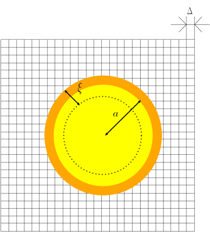
Figure 2: Schematic representation of the cross section of geometry around the rod. $\Delta$ is the lattice spacing, $a$ is the rod radius, and $\xi$ is the interfacial thickness. The rod surface now has a finite volume $\sim 2\pi a\xi$ supported by several grid points on the fixed Cartesian coordinate.

First, the effects of the finite thickness on the drag force are examined in the square domain of $L^{2}$. An uniform stream $U$ in $x$-direction was assigned to the edge of the domain as the boundary condition. Here the Reynolds number was defined by $Re=2aU/\nu$. The drag coefficient was calculated as $C_{D}=F_{D}/\rho U^{2}a$, where the drag force $F_{D}$ was computed from Eq. (26) for various values of $\Delta$, $a$, $L$, and $U$. Figure 3 shows the relative error $\left\{C_{D}(Re,\xi/\Delta)-C_{D}(Re,\xi/\Delta=0)\right\}/C_{D}(Re,\xi/\Delta=0)$ as a function of the interfacial thickness $\xi/\Delta$, where $C_{D}(Re,\xi/\Delta=0)$ was estimated by extrapolating the measured curve of $C_{D}(Re,\xi/\Delta)$ to $\xi/\Delta\to 0$. The relative error in $C_{D}$ was observed to increase with increasing $\xi/\Delta$, however, it tended to converge within $5\%$ for several values of $a/\Delta$ for $\xi/\Delta=1$ and $0<Re<20$. Thus, $\xi/\Delta=1$ was set for further simulations.

Figure 3: The relative error in the drag coefficient $C_{D}$ as a function of the interfacial thickness $\xi/\Delta$.

Next, the drag coefficient $C_{D}$ was calculated. The rod was fixed at the origin in the circular domain with radius $L$. The velocity at the external boundary $r=L$ was set to $\mbox{\boldmath$u$}(r=L,\theta)=U/(1-2\log(a/L))\left[\left\{1-\left(a/L\right)^{2}-2\log\left(a/L\right)\right\}\mbox{\boldmath$e$}_{x}-2\left\{1-\left(a/L\right)^{2}\right\}\cos\theta\mbox{\boldmath$e$}_{r}\right]$ where $\mbox{\boldmath$e$}_{x}$ and $\mbox{\boldmath$e$}_{r}$ are the unit vectors in $x$- and $r$- directions, respectively, and $\tan\theta=y/x$. An analytical solution for the Stokes equation is known for this boundary condition, and the drag force is given by $F_{D}=8\pi\eta U/(1-2\log(a/L))$. The computed $C_{D}$ using the present method as a function of $Re$ is shown in Fig. 4, and is in good agreement with the theoretical Stokes law in $Re\leq 1$ within $5\%$.

Figure 4: Comparisons of the drag coefficient $C_{D}$ (plus) from our method with the theoretical curve of the Stokes law (solid line).

The accuracy of the present method using the finite interfacial thickness $\xi/\Delta=1$ was determined to be acceptable for simulating colloidal dispersions for $Re\leq 1$ based on the numerical results above.

III.2 Sedimentation

The performance of the present method was examined by simulating sedimentation processes of mono-disperse particles in a two dimensional Newtonian fluid in a rectangular box surrounded by non-slip walls with $\rho_{*}=1.1$ and $\alpha=0.143$ The dimensionless parameters were taken to be $Re=0.0916$, $Fr=0.0512$, where the settling velocity and the diameter of particle were taken as the characteristic velocity and length. Other computational parameters were chosen as $\Delta=1$, $\xi/\Delta=1$, $a/\Delta=10$, $L_{x}/\Delta=512$, and $L_{y}/\Delta=1024$, where $y$-axis is in the direction of gravity. In order to prevent the particles from overlapping within the core radius $\simeq a$, the force was added $\mbox{\boldmath$F$}_{i}^{PP}=-\partial E_{PP}/\partial\mbox{\boldmath$R$}_{i}$ due to direct particle-particle interaction using the repulsive part of the Lennard-Jones potential $E_{PP}=0.4\sum_{i=1}^{N-1}\sum_{j=i+1}^{N}\left[\left(2a/R_{ij}\right)^{12}-\left(2a/R_{ij}\right)^{6}\right]\theta(2^{7/6}a-R_{ij}),$ where $\theta(\cdots)$ is the step function and $R_{ij}\equiv\left|\mbox{\boldmath$R$}_{i}-\mbox{\boldmath$R$}_{j}\right|$. The direct interaction $\mbox{\boldmath$F$}_{i}^{PP}$ is not very important when the particles are moving around because the particles never overlap due to the lubrication effect, even without $\mbox{\boldmath$F$}_{i}^{PP}$. Figure 5 shows the lubrication force acting on two approaching rods computed using the present method. The lubrication force is always repulsive in this case, and thus prevents the rods from approaching each other. The strength of the repulsion increases with increasing velocity $U$.

Figure 5: The normalized lubrication force acts on two approaching infinitely long cylindrical rods as a function of the nearest distance between the two surfaces. Different symbols denote different approaching velocities $U$, ranging from $2.5\times 10^{-6}$ to $9.6\times 10^{-2}$ by $U=2.5\times 10^{-6}\times 2.61^{n},~{}n=0\ldots 11$, which almost collapsed. The observed scaling behavior $F=\eta Uf(h)$ with scaling function $f(\dots)$ is characteristic of Stokes flow, due to Reynolds numbers $2aU/\nu<1$.

On the other hand, when the particles are stacked on the bottom wall during the later stage of sedimentation, $\mbox{\boldmath$F$}_{i}^{PP}$ is required to sustain the stacking against gravity. In fact, the repulsion vanishes for immobile pairs of rods.

At the initial configuration, all the particles were placed near the upper wall and both fluid and particle velocities were set to zero, as depicted in Fig. 6(a). A typical snapshot during sedimentation is shown in Fig. 6(b). Regions with swirled particles were observed, in which the particle velocities were highly correlated as a result of long-range inter-particle hydrodynamic interactions. A simulation with periodic boundary conditions in the horizontal ($x$-)direction was also conducted. In this simulation, swirls were still developed, however they were smaller than those observed with non-slip walls. The effect of confinement in the non-slip walls therefore enhances the velocity correlation. The computational demand required for the present simulation is less than one day of processing on a normal PC.

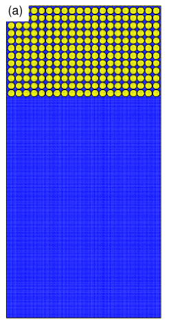
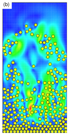
Figure 6: Snapshots of 240 colloidal disks sedimenting in a two-dimensional Newtonian fluid obtained using the present method. The magnitude of the host fluid velocity is indicated in color; change of color from blue to red corresponds to change of the fluid velocity from small to large.

IV Concluding Remarks

A new computational method has been developed to simulate particle dispersion in fluids. Utilizing a smoothed profile for solid-fluid boundaries, hydrodynamic interactions in many particle dispersions can be taken fully into account, both accurately and efficiently. In principle, the present method can be easily applied to systems consisting of many particles with any shape. The reliability of the method was examined by calculating the drag force acting on a cylindrical object in a flow. The performance of the method was demonstrated to be satisfactory by simulating sedimentations of particles in a Newtonian fluid.

Another primary benefit of using the smoothed profile arose when the method was extended to colloidal dispersions in complex fluids with an internal degree of freedom, such as the molecular orientation or ionic density. In complex fluids, inter-particle interactions can be mediated by the internal degree of freedom of the fluid. In such cases, the fluid-particle interactions at the colloid surface could be more efficiently handled by utilizing a smoothed profile. Previous studies on particle dispersions in liquid crystal solvents demonstrate a striking example of this efficiency Yamamoto (2001); Yamamoto et al. (2004). Although the hydrodynamic effects were neglected in these simulations, extensions to implement the hydrodynamic effects by incorporating the present method are currently underway.

Appendix A Selection of smoothed profiles

The specific form of the smoothed profile should be selected according to the convenience of the physical modeling of systems under consideration. In the present study, an infinitely differentiable function with compact support was used. We adopted $\phi$ defined as

$$\phi_{i}(\mbox{\boldmath$x$}) = g(\left|\mbox{\boldmath$x$}-\mbox{\boldmath$R$}_{i}\right|),$$ (31)

$$g(x) = \frac{h((a+\xi/2)-x)}{h((a+\xi/2)-x)+h(x-(a-\xi/2))},$$ (32)

$$h(x) = \left\{\begin{array}[]{cc}\exp\left(-\Delta^{2}/x^{2}\right)&x\geq 0,\\ 0&x<0.\end{array}\right.$$ (35)

where $\mbox{\boldmath$R$}_{i}$, $a$, $\xi$, and $\Delta$ were the position of the particle, the radius of the particle, the interfacial thickness, and lattice spacing, respectively. This choice is shown in Fig. 2. While this $\phi$ may appear somewhat complicated compared to other more simple choices, this $\phi$ has the following benefits: i) three domains; solid, fluid, and interface are explicitly separated, namely, $\phi=1$ is the solid domain ($\left|\mbox{\boldmath$x$}-\mbox{\boldmath$R$}_{i}\right|<a-\xi/2$), $\phi=0$ is the fluid domain ($a+\xi/2<\left|\mbox{\boldmath$x$}-\mbox{\boldmath$R$}_{i}\right|$), and $0<\phi<1$ is the interfacial domain ($a-\xi/2<\left|\mbox{\boldmath$x$}-\mbox{\boldmath$R$}_{i}\right|<a+\xi/2$), ii) high order derivatives of $\phi_{i}$ with respect to $x$ can be analytically calculated, and iii) due to its support-compactness, the integrals in Eqs. (26) and (27) remain local, which contributes greatly to the efficiency of the computation.

The second possible choice is

$$\phi_{i}(\mbox{\boldmath$x$}) = \frac{1}{2}\left(\tanh\frac{a-\left|\mbox{\boldmath$x$}-\mbox{\boldmath$R$}_{i}\right|}{\xi}+1\right).$$ (36)

This choice was used in Refs Tanaka and Araki (2000); Yamamoto (2001); Yamamoto et al. (2004). This $\phi$ is also infinitely differentiable as well as analytically easy to handle. However, the support is not compact and the separation of the three domains is ambiguous. Furthermore, the ambiguity of domain separation tends to be more enhanced for higher order derivatives. For practical implementation, due to exponential decay of the hyperbolic function, a proper cutoff radius is adopted for the calculation of the integrals in Eqs. (26) and (27).

The third possible choice is given by

$$\phi_{i}(\mbox{\boldmath$x$}) = s(a-\left|\mbox{\boldmath$x$}-\mbox{\boldmath$R$}_{i}\right|),$$ (37)

$$s(x) = \left\{\begin{array}[]{cc}0&x<-\xi/2,\\ \frac{1}{2}\left(\sin\frac{\pi x}{\xi}+1\right)&\left|x\right|<\xi/2,\\ 1&x>\xi/2.\end{array}\right.$$ (41)

which has the property of exact separation of the three domains, however, the second derivative of $\phi$ is discontinuous at the fluid-interface boundary. Therefore, it is not recommended for computational models requiring derivatives higher than the second order of $\phi$.

The detailed choice of $\phi$ does not affect the results of the present simulations because only the first order derivative of $\phi$ is required in the present case. However, care must taken if higher order derivatives are required.

References

- Russel et al. (1989) W. B. Russel, D. A. Saville, and W. R. Schowalter, Colloidal Dispersions (Cambridge University Press, Cambridge, 1989).
- Larson (1999) R. G. Larson, The Structure and Rheology of Complex Fluids (Oxford University Press, New York, 1999).
- Segré et al. (2001) P. N. Segré, F. Liu, P. Umbanhowar, and D. A. Weitz, Nature 409, 594 (2001).
- Stark (2001) H. Stark, Phys. Rep. 351, 387 (2001).
- Tanaka (1999) H. Tanaka, Phys. Rev. E 59, 6842 (1999).
- Winslow (1949) W. M. Winslow, J. Appl. Phys. 20, 1137 (1949).
- Brady and Bossis (1988) J. F. Brady and G. Bossis, Ann. Rev. Fluid Mech. 20, 111 (1988).
- Ichiki (2002) K. Ichiki, J. Fluid Mech. 452, 231 (2002).
- Glowinski et al. (2001) R. Glowinski, T. W. Pan, T. I. Hesla, D. D. Joseph, and J. Périaux, J. Comput. Phys. 192, 363 (2001).
- Höfler and Schwarzer (2000) K. Höfler and S. Schwarzer, Phys. Rev. E 61, 7146 (2000).
- Yamamoto (2001) R. Yamamoto, Phys. Rev. Lett. 87, 075502(4) (2001).
- Yamamoto et al. (2004) R. Yamamoto, Y. Nakayama, and K. Kim, J. Phys.: Condens. Matter 16, S1945 (2004).
- Succi (2001) S. Succi, The lattice Boltzmann equation for fluid dynamics and beyond (Clarendon Press, Oxford, 2001).
- Ladd and Verberg (2001) A. Ladd and R. Verberg, J. Stat. Phys. 104, 1191 (2001).
- Tanaka and Araki (2000) H. Tanaka and T. Araki, Phys. Rev. Lett. 85, 1338 (2000).
- Kajishima et al. (2001) T. Kajishima, S. Takiguchi, H. Hamasaki, and Y. Miyake, JSME Int. J., Ser. B 44, 526 (2001).