Heterogeneity, and the secret of the sea

Abstract

This paper explores tools for modeling and measuring the compositional heterogeneity of a rock, or other solid specimen. Intuitive “variation per decade” plots, simple expressions for containment probability, generalization for familiar error-in-the-mean expressions, and a useful dimensionless sample bias coefficient all emerge from the analysis. These calculations have also inspired subsequent work on log-log roughness spectroscopy (with applications to scanning probe microscope data), and on angular correlation mapping of lattice fringe images (with applications in high resolution transmission electron microscopy). It was originally published as Appendix E of a dissertationFraundorf (1980) on “Microcharacterization of interplanetary dust collected in the earth’s stratosphere”.

I 2nd moment statistics: next after mean

An intuitively simple, but quantitative, approach to spatial heterogeneity is possible using mathematics which claims wide familiarity because of its already diverse applications. The composition of a specimen can be considered a function of spatial position whose statistical properties are fully described by a set of underlying probability distributionsWang and Uhlenbeck (1945). These distributions are fully specified by knowledge of their moments. Naturally, the first parameters to measure in describing these distributions are the first moments: the average values or compositional abundances. Elemental and mineral (modal) abundances have long been familiar tools in the characterization of geological specimens.

The logical next step in specifying the distributions is to use information on point-to-point variations to measure the second moments of the probability distributions. If, for simplicity and in the interest of improved sample statistics, the underlying distributions are considered invariant under translations and rotations, then the statistics of point-to-point variations are fully described by the set of one-parameter functions known as radial covariances. If these functions are measured (using a three-dimensional array of sample points) for a specimen whose distributions are not invariant under rotations and translations (e.g. in samples with aligned crystals or a compositional gradient), then these functions will represent averages (over direction and position) of covariance functions which depend on orientation and absolute position in the sample. Of course, if one wishes to infer statistical properties of the parent material from a laboratory sampling, it is necessary (and traditional) to assume translational invariance in the absence of contrary information. Because inferences from samples volume to the larger specimen are an important aspect here, a definition of source material extending only to material in which the underlying distributions are “stationary” will be implicit in the discussion to follow. Rotational invariance (or isotropy) for the underlying distributions will not be taken for granted, although its assumption will be necessary if one wishes to measure the radial covariances from polished sections which do not sample a wide variety of orientations in the specimen.

Applications for the concept described above are most familiar in the field of time series analysisBlackman and Tukey (1959); Bloomfield (1976), where the one-dimensional independent variable, time, is used in place of the three-dimensional variable, position. However, the concept itself is quite general, and myriad two and three dimensional spatial applications already exist in the literatureWu (1972); Peebles (1973). In fact, curiousity about the statistical properties of composition in rocks was inspired with an article by Martin GardnerGardner (1978) concerning applications to natural phenomena ranging from the topology of cratered terrainMandelbrot (1977) to the pattern of notes and rhythm in a piece of musicVoss and Clark (1975).

The general covariance function (or cross-covariance) of variables $A$ and $B$ evaluated at regions displaced by $\Delta\vec{x}$ is defined by

$$\sigma_{AB}[\Delta\vec{x}]\equiv\langle\{A[\vec{x}+\Delta\vec{x}]-\mu_{A}\}\{B[\vec{x}]-\mu_{B}\}\rangle_{\vec{x}}.$$ (1)

Conventional notation will be used here: population (or “parent specimen”) averages are denoted by angle brackets $\langle\rangle$ or Greek letters, while sample (i.e. measured) averages are denoted by a bar over the quantity, or Roman letters. In particular, $\mu_{A}$ and $\mu_{B}$ are defined as the population averages of $A$ and $B$ respectively, with the averages here taken over all possible values of location vector $\vec{x}$. Note: This quantity is sometimes put into dimensionless (correlation coefficient) form by normalizing with standard deviations of $A$ and $B$, as in $\rho_{AB}[\Delta x]\equiv\frac{\sigma_{AB}[\Delta x]}{\sigma_{A}\sigma_{B}}$.

For the petrographic application, it is useful to examine a mixture of $n$ homogeneous phases. Consider spatial heterogeity for the variables $A$ and $B$ which take on values of ${}_{i}A$ and ${}_{i}B$, respectively, in the ith phase, $i=1,n$. If $p[i,j,t]$ is the joint probability that, for two sample points separated by a distance (or lag) $t$, the first will lie on a phase $i$ region and the second will lie on a phase $j$ region, then the radial covariance function for $A$ and $B$ can be written:

$$\sigma_{AB}[t]=\sum\limits_{i=1}^{n}{\sum\limits_{j=1}^{n}{p[i,j,t]({}_{i}A-\mu_{A})({}_{j}B-\mu_{B})}}.$$ (2)

If $A\equiv B$, then the quantity defined above is referred to as the radial auto-covariance for $A$.

The $\sigma_{AB}[t]$ constitute a measure of the statistical correlation between the value of the parameters $A$ and $B$ at points in the specimen separated by a distance $t$. For the special case $t=0$, the radial covariance $\sigma_{AB}[t]$ reduces to the covariance for $A$ and $B$ in the specimen, i.e. $\sigma_{AB}[0]=\sigma_{AB}$. Similarly the radial auto-covariance for $A$, $\sigma_{AA}[t]$, reduces to the variance of $A$ in the specimen, i.e. $\sigma_{AA}[0]={\sigma_{A}}^{2}$. Using this notation, the absolute value of $\sigma_{AB}[t]$ for the specimen is less than or equal to the product of standard deviations $\sigma_{A}\sigma_{B}$, and it is equal to zero when values of $A$ and $B$ measured at points separated by length $t$ are uncorrelated.

Although the general covariance functions contain all information on the statistics of point-to-point variations in a specimen, the value of the function at any chosen argument depends upon heterogeneities that may have many different length scalesPeebles (1973). Fortunately, knowledge of covariance functions can be converted, without loss of detail, to knowledge of spectral densities which serve to separate effects due to heterogeneity on various size scales. In this way, data obtained by techniques which are sensitive to heterogeneity on different size scales can be combined to provide a picture of compositional variability over a wide range of spatial frequencies.

If we mimic equation 1 and define correlation $C_{AB}[\Delta\vec{x}]$ as the average over all $\vec{x}$ of $A$ times $B$ at regions displaced by $\Delta\vec{x}$, one can quite generally write $\sigma_{AB}=C_{AB}-\mu_{A}\mu_{B}$, where the product of the means is a constant with no dependence on $\Delta\vec{x}$. But the Fourier correlation theoremPress et al. (1992) says that correlation is the inverse transform of the conjugate product of spectral densities for $A$ and $B$ in the specimen, and $\mu_{A}$ and $\mu_{B}$ are volume-normalized spectral densities measured at zero frequency. Thus the Fourier transform of $\sigma_{AB}$ is the conjugate product of volume-normalized spectral densities for $A$ and $B$, with the zero-frequency value set to zero.

To be specific, equation 2 defines a function of the magnitude of the separation between two points in the sample, but not of the direction of that separation. Its three-dimensional Fourier transform (using signal processing conventions) can be written as:

$$\gamma_{AB}[f]\equiv 2\int\limits_{0}^{\infty}{\frac{t}{f}}\sin[2\pi ft]C_{AB}[t]dt.$$ (3)

The inverse equation for this expression is:

$$C_{AB}[t]\equiv 2\int\limits_{0}^{\infty}{\frac{f}{t}}\sin[2\pi ft]\gamma_{AB}[f]df.$$ (4)

For the case $t=0$, this yields the relationships:

$$C_{AB}[0]\equiv\int\limits_{0}^{\infty}4\pi{f^{2}}\gamma_{AB}df=\int\limits_{-\infty}^{\infty}{4\pi f^{3}}\gamma_{AB}d(\ln f).$$ (5)

Hence one might relate spectral density physically to $4\pi{f^{2}}\gamma_{AB}$, which from above is that portion of the covariance $\sigma_{AB}[0]=C_{AB}[0]-\mu_{A}\mu_{B}$ resulting from compositional fluctuations occurring with spatial frequency in the interval from $f$ to $f+df$. For a quantity independent of the units used to measure frequency, the second equality in 5 relates spectral density to $4\pi{f^{3}}\gamma_{AB}$, that portion of the covariance between $A$ and $B$ in a given “e-fold” of frequency (or decade of frequency should one further multiply by $\ln 10$).

One example is the special case when all variations occur with one frequency, $f_{o}$. Sinusoidal banding of an otherwise homogeneous material would, for instance, give rise to this condition. Regardless of details of the underlying distribution, however, the radial auto-covariance and spectral-density (sans origin) for a variable of this type can be written:

$$\sigma_{AA}[t]\equiv\sigma_{A}^{2}\frac{{\sin[2\pi f_{o}t]}}{{2\pi f_{o}t}},$$ (6)

and

$$\gamma_{AA}[f]\equiv\sigma_{A}^{2}\frac{{\delta[f-f_{o}]}}{{4\pi f_{o}^{2}}}.$$ (7)

II The well-mixed model

Although long-range order, like that described by equations 6 and 7, is certainly possible in geological materials (e.g. in compositional zoning of mineral single crystals), it is likely to be the exception rather than the rule in most aggregate materials. A more likely model is one which assumes that the specimen consists of single-phase regions whose relative positions are fully random (that is, well-mixed) with respect to one another. If the regions are atomic dimensions in size, then the model describes a glass; if the single-phase regions are considerably larger, then the model would describe, for example, a well-mixed breccia. In igneous or metamorphosed materials, the possibility of compositional correlations between adjacent crystals could give rise to deviations from this well-mixed case.

Even a well-mixed model could be quite difficult analytically if one wishes to consider the details of the interplay (in three dimensions) between grain shapes, sizes, and the packing arrangement. However, considerable simplification results if one assumes short range order in the sense that lage, which leave their initial grain, necessarily terminate on points compositionally uncorrelated with the starting location. If we define $p[i]$ as the fractional abundance of phase $i$ points, and $\xi_{i}[t]$ as the probability that lag $t$, beginning at an arbitrary location on a grain of type $i$, will not leave that grain before ending, then we can write:

$$\sigma_{AB}[t]=\sum\limits_{i=1}^{n}{p[i]({}_{i}A-\mu_{A})}({}_{i}B-\mu_{B})\xi_{i}[t],$$ (8)

and

$$\gamma_{AB}[f]=\sum\limits_{i=1}^{n}{p[i]({}_{i}A-\mu_{A})}({}_{i}B-\mu_{B})\Xi_{i}[f].$$ (9)

The function $\Xi_{i}[f]$ is the radial Fourier transform of the containment probability $\xi_{i}[t]$, which in turn obeys the simple constraint:

$$4\pi\int\limits_{0}^{\infty}{\xi_{i}[t]t^{2}dt=\Xi_{i}[0]=\langle V_{i}}\rangle,i=1,n.$$ (10)

Here, $\langle V_{i}\rangle$ is the (volume-weighted) average volume for grains of type $i$.

Calculations for several simple grain geometries have been attempted. For spherical grains of diameter $D$, the containment probability isPlachy (1980):

$$\xi_{i}[t]=\{\begin{array}[]{*{20}c}{1-\frac{3}{2}\left({\frac{t}{D}}\right)+\frac{1}{2}\left({\frac{t}{D}}\right)^{3}}&{,t\leq D.}\\ 0&{,t>D.}\\ \end{array}$$ (11)

Of course, not only are truly spherical grains rare, but a model made up solely of spheres of one size necessarily is filled with voids.

A more realistic model for containment probabilities comes from the case of rectangular solids. Unfortunately, a full analytical solution has not yet been obtained. The case for a cube of side $d$ has been tabulated by a combination of analytical and numerical methods. Somewhat by accident it was discovered that an RMS deviation from the exact values of only 0.0045, over the non-zero range $0<t<\sqrt{3}d$, is obtained with the much simpler approximation:

$$\xi_{i}[t]\cong\{\begin{array}[]{*{20}c}{\left(1-{\frac{t}{{bd}}}\right)^{2}}&{,t\leq bd.}\\ 0&{,t>bd.}\\ \end{array}$$ (12)

Here $b$, from the volume constraint 10, must equal $\left({\frac{30}{4\pi}}\right)^{1/3}$. The Fourier transform of the approximation is also similar to the exact one, although the low level “ripples” for values of $f$ large compared to $1/d$ are differently placed. These ripples are of course averaged away when a continuum of grain sizes are used, and hence should have no effects in applications to real materials. Thus the approximation given in 12 for a cube of side $d$ will be adopted as a simple expression for work here.

The equation 8 provides a model for mixed-grain radial covariances, given the phase abundances $p[i]$ and the containment probability function $\xi_{i}[t]$ for grains of each phase. Note that in this well-mixed case, auto-covariance will always be a positive monotone-decreasing function of lag which goes to zero for lags large compared to “compositional” grain sizes in the specimen. In particular, if the grain geometry (in terms of the containment probability function) is the same for all phases, then all of the $\sigma_{AB}[t]$ for the specimen exhibit the same $t$ dependence. For such a specimen, knowledge of the $t$ dependence for the radial auto-covariance of one variable would specify the $t$ dependence for all. Conversely, if the $n$ phases obey one of $m$ different containment probability functions ($m\leq n$), then measurement of the radial auto-covariance for $m$ variables might allow calculation of the containment probabilities for each phase type via 8, as well as a check of the model by predicting values of the radial cross-covariances (i.e. cases in which $A\neq B$).

Given that many geological samples can be considered neither homogeneous glasses nor well-mixed breccias, then what deviations from the well-mixed model are to be expected? One simple deviation can be detected by checking the relationship between physical grain size and compositional grain size. If the two do not agree, then a more complicated history is required. For example, a physical grain size much smaller than the compositional grain size might result from a breccia composed of larger fragments which were crushed by not well-mixed prior to compaction. Conventional petrographic analysis, unsurpassed in its ability for qualitative discernment of patterns requiring knowledge of higher statistical moments, would be helpful in verifying the cause even if the effect itself required the quantitative approach described here.

In a wider variety of ways, well-mixed materials can be modified by open and closed-system thermodynamic processes. If the scale of transport allowed in such processes is large compared to the sample size, especially in the presence of a long-range gravitational force, then the resulting effects on specimen heterogeneity must be handled case by case. But if in-situ transport processes are limited to distances smaller than the specimen size, then one overall effect of the redistribution of material is predictable: regions enriched on one element will be surrounded by regions depleted in that element. This means that the probability of finding such a redistributed element is likely to decrease upon leaving an enriched region, prior to leveling off at the average probability. Hence the radial auto-covariance for that element is likely to go below zero before it dies out as $t$ gets larger. In the limiting case when an element-pure region (phase 1) is small compared to a surrounding element-free region (phase 2), then the negative excursion for $\sigma_{AA}[t]$ goes down to:

$$min[\sigma_{AA}[t]]\cong-\left(\frac{b_{1}}{b_{2}}\right)^{3}\sigma_{A}^{2}.$$ (13)

Here $b_{1}$ is a characteristic dimension of the enriched zone and $b_{2}$ a typical size for the depleted zone.

The possibly diagnostic nature of such deviations from the well-mixed case suggests that measurement of these quantities from actual samples, in addition to modeling on the basis of the observation of phase abundances and geometries, might be a worthwhile pursuit. This is especially true in light of the fact that information on point-to-point compositions in geological materials is frequently available, and the data on relative locations of the sampled points easy to obtain, during the course of automated modal analyses.

III Measurement from compositional data

Compositional information, as a function of position in a specimen, is most conveniently measured on flat sections of the specimen. This is true whether compositional identifications are made by optical microscopy, polished-section energy or wavelength dispersive x-ray analysis, or thin-specimen analytical transmission electron microscopy. As mentioned at the outset, measurement of radial covariances from “two-dimensional” samples of this sort requires either (1) an assumption that the specimen analyzed is isotropic, or (2) averaging of the data for sections which sample a wide range of orientations in the specimen. A third alternative is to use slices through the specimen taken in a why such that the relative three-dimensional positions of the sampled locations are known. Observations of the chondritic interplanetary dust aggregates examined in this thesis, with SEM and TEM, provide no indication that the assumption of radial isotropy is unwarranted at this point.

As will be easier to see in examples of the Fourier transformed radial covariances, the spatial resolution of the sampling method and the maximum separation between points considered in the covariance calculation determine, respectively, the upper and lower bounds (in terms of spatial frequency) on the “spectral window” through which specimen heterogeneity is being examined. In order to avoid aliasing it is useful to set the minimum spacing between analysis points (the “lag interval”) to be on the order of (or smaller than) the spatial resolution of the point analyses. In order to improve spectral resolution and increase the number of effectively independent sample locations, it is important to sample as wide a range of lags (point separations) as is possible. In meeting these criteria for a fixed number of point analyses, a simple square array of sampled locations is not the optimum configuration, but it is one which will be frequently encountered. In the discussion to follow, we will assume quite generally an array of $M$ sample locations: $A_{i}$ and $B_{i}$ are the values measured for $A$ and $B$ at the ith sample location (position $\vec{x}_{i},i=1,M$). Thus the postscripts on $A$ and $B$ refer to sampled locations, not to mineral phases.

Although a number of slightly different “sample” cross-covariance functions could be defined, it is simplest in the interest of subsequent error analysis to use for $\mu_{A}$ and $\mu_{B}$ the best available estimates for the mean values of $A$ and $B$ in the specimen, and then to calculate:

$$s_{AB}[t]\equiv\left({\frac{1}{M_{t}}}\right)\sum\limits_{i=1}^{M}{\sum\limits_{j=1}^{M}{\delta_{tij}(A_{i}-\mu_{A})}}(B_{j}-\mu_{B}).$$ (14)

Here $\delta_{tij}$ is simply a delta function used to disallow from the double sum all terms except those for which analysis points $i$ and $j$ are separated by a distance $t$ in the specimen, and $M_{t}$ is just the double sum over that delta function (i.e. the number of point pairs in the sample separated by a distance $t$). Of course, any two or three dimensional sample configuration is likely to include pairs which are not all integral multiples of the (minimum) lag interval, $\Delta t$. In order to create a set of equally spaced data points for the Fourier transform process, it is useful to “widen” $\delta_{tij}$ to allow all pairs into the sums for $t$ which have separations within $\frac{1}{2}\Delta t$ on either side of $t$, and then to evaluate 14 for all $t_{j}=(j-\frac{1}{2})\Delta t,j=1,T/\Delta t$. Here $T$ is the maximum lag introduced into the calculation. Because of the large uncertainties associated with data on lags larger than half of the sample size, $T$ will usually be chosen to be less than half of the maximum separation between points in the sample.

As with any estimate of the radial covariance based on measurements from a finite sample, 14 provides a biased estimate. If we define restricted averages, based only on data pairs separated by the distance $t$, of the form:

$$\bar{A}_{t}\equiv\left({\frac{1}{{M_{t}}}}\right)\sum\limits_{i=1}^{M}{\sum\limits_{j=1}^{M}{\delta_{tij}A_{i}}},$$ (15)

then with simple algebra it is easy to verify that:

$$\langle s_{AB}[t]\rangle=\sigma_{AB}[t]-\langle(\bar{A}_{t}-\mu_{A})(\bar{B}_{t}-\mu_{B})\rangle.$$ (16)

If lags of all sizes are uniformly distributed over the sample, then the second term in 16 will depend very little on $t$, and be approximately equal to $\langle(\bar{A}-\mu_{A})(\bar{B}-\mu_{B})\rangle$, the covariability in estimates of $\mu_{A}$ and $\mu_{B}$ from the sample. Thus when $A\equiv B$, the probable bias in the estimate 14 is just the variance in the estimate of $\mu_{A}$, which cannot be determined without assumptions about the character of the parent specimen (see next section). The amount of bias is roughly the same for all $t$, and hence 14 provides an unbiased estimate for the shape of $\sigma_{AB}[t]$, but not for its absolute position in the vertical direction. On the other hand, the bias in estimates of the spectral density is not independent of frequency. Before estimation of the spectral density, however, the abrupt cutoff in the radial covariance estimate at $t=T$ must be addressed.

In order to avoid forcing the calculated covariance function $s_{AB}[t]$ abruptly to zero for $t\geq T$, it is traditionalBlackmank59 to do this gradually prior to Fourier transformation by multiplying the measured covariance function by a function which goes “gently” from 1 down to zero over the interval $0<t<T$. A common choice of this function is the Hanning lag window, defined by:

$$D[t]=\{\begin{array}[]{*{20}c}{{\textstyle{1\over 2}}(1+\cos[{\textstyle{{\pi t}\over T}}])}&{,t\leq T}\\ 0&{,t>T}\\ \end{array}$$ (17)

The finite range of lags allowed into the calculation for $S_{AB}[t]$ inevitably decreases the resolution of the measured spectral density. Gentle supression of the covariance function for large lags prior to Fourier transformation results in a simple “blurring” of details from the spectral density function. Without this “smooth” window, the loss of resolution would occur in a more complicated way.

If we define the number of terms in the calculation: $N\equiv T/\Delta t$; and the discrete frequencies $f_{k}=(k-{\textstyle{1\over 2}})/(2T),k=1,N$; then we can write the three dimensional digital transforms (following 3 and 4) as:

$$g_{AB}[f_{k}]=\frac{{\left({\Delta t}\right)^{2}}}{T}\sum\limits_{j=1}^{N}{\frac{{t_{j}}}{{f_{k}}}}s_{AB}[t_{j}]D[t_{j}]\sin[2\pi f_{k}t_{j}],$$ (18)

for $k=1,N$, and conversely for $j=1,N$:

$$s_{AB}[t_{j}]D[t_{j}]=\frac{2}{{\Delta t}}\sum\limits_{j=1}^{N}{\frac{{f_{k}}}{{t_{j}}}}g_{AB}[f_{k}]\sin[2\pi f_{k}t_{j}].$$ (19)

To examine bias in the spectral density estimate, the discrete transform of 16 can be taken. Again if the lags are uniformly distributed over the sample volume, then to first order this can be written:

$$\langle g_{AB}[f]\rangle=\gamma_{AB}[f]-\langle(\bar{A}-\mu_{A})(\bar{B}-\mu_{B})\rangle\sum\limits_{j=1}^{N}{\frac{{t_{j}}}{f}\sin[2\pi ft_{j}]}.$$ (20)

The summation term in this equation is the discrete approximation to a delta function at the origin. That is, it is very large for $f\simeq 0$, but very small for other values of $f$. The upshot of this is that the spectral density estimate is likely to be seriously biased due to uncertainty in the specimen averages only for $f\geq(1/T)$. For aspects of the estimates for which bias due to the finite sample is not a problem, the analysis of uncertainties is straightforward if $A$ and $B$ are assume to be Gaussian variatesBlackman and Tukey (1959). As mentioned above, one result of such analysis is that large uncertainties are associated with data on lags larger than half the sample size. These uncertainties result in large uncertainties for all frequencies in the spectral density estimate. Thus making the maximum lag allowed into the calculation ($T$) small compared to the sample size has two effects on the spectral density estimates: It decreases spectral resolution but at the same time increases the stability of spectral density estimates for all frequencies.

IV The statistics of sampling

Suppose one measures the variable $A$ at $M$ points on a specimen, and wishes to determine an average value for $A$ in that specimen. The $M$ analysis “points” constitute the sample. Standard practice is to calculate the sample mean from the measured values for $A$:

$$\bar{A}\equiv\frac{1}{M}\sum\limits_{i=1}^{M}{A_{i}.}$$ (21)

This value $\bar{A}$ constitutes an “unbiased” estimate for the specimen (or “population”) mean $\mu_{A}$ since the expected value for this measurement is indeed the population avearge, i.e.:

$$\langle\bar{A}\rangle\equiv\mu_{A}.$$ (22)

The object of this section is to provide a prediction for the error in this estimate. To see how this error will depend on specimen heterogeneity, one need only consider the case in which all $M$ analysis points are clustered into a tiny volume much smaller than the grain size of a rock. One would hardly expect to learn much about the composition of the whole rock from such an analysis, regardless of the size of $M$. On the other hand, if the analysis points are randomly spread out over distances much larger than the average grain size, then for $M$ sufficiently large it should be possible to determine the rock composition arbitrarily well. A nice feature of the approach adopted here is that the resulting answer will require no assumption about the random mixing of the constituent grains. It instead follows simply from the definition of radial covariance.

The expected value for variance in the estimate of $\mu_{A}$ from measurements on the sample of $M$ points is:

$$\langle(\bar{A}-\mu_{A})^{2}\rangle\equiv\frac{1}{{M^{2}}}\sum\limits_{i=1}^{M}{\sum\limits_{j=1}^{M}{\langle(A_{i}-\mu_{A})(B_{j}-\mu_{B})\rangle}}$$ (23)

where the term in the summations is none other than $\sigma_{AA}[t_{ij}]$, i.e. the radial variance for separations $t_{ij}$ between ith and jth sample locations. Thus the variance in estimates of the mean is just the average of radial auto-covariance for data from pairs of points in the sample. In a similar fashion, an estimate of the covariance between sample estimates of $\mu_{A}$ and $\mu_{B}$ can be written as:

$$\langle(\bar{A}-\mu_{A})(\bar{B}-\mu_{B})\rangle\equiv\frac{1}{{M^{2}}}\sum\limits_{i=1}^{M}{\sum\limits_{j=1}^{M}{\sigma_{AB}[t_{ij}]}}.$$ (24)

Thus knowledge of the radial covariance functions for a given specimen allows prediction of the uncertainty in estimates of means based on measurements from a limited sample.

The way in which sample size and compositional coarseness modifies estimates of uncertainty in the mean can be seen more clearly if the “i=j” terms are separated from the double sum in equation 23. One can then write:

$$\langle(\bar{A}-\mu_{A})^{2}\rangle=\{1+(M-1)\rho\}\frac{{\sigma_{A}^{2}}}{M}=\{\begin{array}[]{*{20}c}{\frac{1}{M}{\sigma_{A}^{2}}}&{,\left|\rho\right|\ll\frac{1}{M}}\\ {}\hfil&{}\hfil\\ {\rho\sigma_{A}^{2}}&{,\left|\rho\right|\gg\frac{1}{M}}\\ \end{array}$$ (25)

where a sample bias coefficient for the sample configuration has been defined as an average over all pairs of sample points by:

$$\rho\equiv\frac{1}{{M(M-1)}}\sum\limits_{i=1}^{M}{\sum\limits_{j\neq 1}^{M}{\frac{{\sigma_{AA}[t_{ij}]}}{{\sigma_{AA}[0]}}.}}$$ (26)

This sample bias coefficient is to first order dependent only upon the lag dependence of the covariance function for $A$, and on the sample size. It, like the radial covariance function, is expected to approach zero for sample locations which are widely separated. Hence, for sufficiently large sample regions, equation 25 predicts that sample analysis points can be considered independent of one another. By the same token, however, for a sample of fixed size, an increase in the number of analysis points beyond $M\simeq\left|1/\rho\right|$ buys little decrease in uncertainty.

If one wishes to estimate $\sigma_{A}^{2}$ from the same limited-sample measurement, the increase in uncertainty due to a sample which is too localized is even more severe. If one measures the sample variance:

$$s_{A}^{2}\equiv\frac{1}{M}\sum\limits_{i=1}^{M}{(A_{i}-\bar{A})^{2}},$$ (27)

then an unbiased estimate for $\sigma_{A}^{2}$ is obtained from the relation:

$$\sigma_{A}^{2}=\left({\frac{M}{{M-1}}}\right)\frac{{\langle s_{A}^{2}\rangle}}{{1-\rho}}\cong\{\begin{array}[]{*{20}c}{{\textstyle{M\over{M-1}}}\langle s_{A}^{2}\rangle}&{,\left|\rho\right|\ll{\textstyle{1\over M}}}\\ {}\hfil&{}\hfil\\ {{\textstyle{1\over{1-\rho}}}\langle s_{A}^{2}\rangle}&{,\left|\rho\right|\gg{\textstyle{1\over M}}}\\ \end{array}$$ (28)

Equation 25 can then be written as:

$$\langle(\bar{A}-\mu_{A})^{2}\rangle=\frac{{1+(M-1)\rho}}{{(M-1)(1-\rho)}}\langle s_{A}^{2}\rangle,$$ (29)

which in the limits becomes

$$\langle(\bar{A}-\mu_{A})^{2}\rangle\cong\{\begin{array}[]{*{20}c}{{\textstyle{1\over{M-1}}}\langle s_{A}^{2}\rangle}&{,\left|\rho\right|\ll{\textstyle{1\over M}}}\\ {}\hfil&{}\hfil\\ {{\textstyle{\rho\over{1-\rho}}}\langle s_{A}^{2}\rangle}&{,\left|\rho\right|\gg{\textstyle{1\over M}}}\\ \end{array}$$ (30)

Again, these values equal those for independent sample locations if $\left|\rho\right|$ is sufficiently small. However for a sufficiently small sampled region, $\rho$ approaches one and even hundreds of analysis points on such a small sample cannot result in reasonable uncertainties for our estimate of $\mu_{A}$.

For the case when the sampled region is not a set of discrete points but a continuous sampled volume, then two simplifications ensue. First, the number of analysis points $M$ effectively goes to infinity, so that the limiting cases of equations 25 and 30 apply for which $\left|\rho\right|\gg\frac{1}{M}$. Secondly, equation 26 can be rewritten:

$$\rho={\textstyle{{4\pi}\over V}}\int\limits_{0}^{\infty}{\frac{{\sigma_{AA}[t]}}{{\sigma_{AA}[0]}}\xi[t]t^{2}dt=}{\textstyle{{4\pi}\over V}}\int\limits_{0}^{\infty}{\frac{{\gamma_{AA}[f]}}{{\sigma_{AA}[0]}}\Xi[f]f^{2}df.}$$ (31)

Here $\xi[t]$ is the containment probability defined in section II, but this time with reference to the sample volume $V$ instead of a grain volume. As before, $\Xi[f]$ is the radial Fourier transform of $\xi[t]$. When viewed in this light, the quantity $\xi[t]/V$ is just the probability of two points in the sample being separated by distance $t$, per unit volume increment $4\pi t^{2}dt$. The integration constraint 10 becomes:

$$4\pi\int\limits_{0}^{\infty}{\frac{{\xi[t]}}{V}t^{2}dt}=\frac{{\Xi[0]}}{V}=1.$$ (32)

Because of the presence of $V$ in the denominator of equation 31, a sample bias coefficient can also be calculated for two-dimensional and one-dimensional sample arrays.

For the purpose of this study, the most welcome facet of equation 31 is that the cube approximation of 12 can be utilized for both $\xi[t]$ and for $\sigma_{AA}[t]/\sigma_{AA}[0]$, in one case with reference to the sample volume and in the second case with reference to the specimen grain size, to provide a good general purpose estimate of sample bias coefficient as a function of sample size $D$ and grain size $d$:

$$\rho\left[{\frac{D}{d}}\right]\cong\{\begin{array}[]{*{20}c}{1-\left({\frac{D}{d}}\right)+\frac{2}{7}\left({\frac{D}{d}}\right)^{2}}&{,D\leq d}.\\ {}\hfil&{}\hfil\\ {\left({\frac{d}{D}}\right)^{3}-\left({\frac{d}{D}}\right)^{4}+\frac{2}{7}\left({\frac{d}{D}}\right)^{5}}&{,D>d}.\\ \end{array}$$ (33)

Appendix A Heterogeneity of interplanetary dust

One of the qualitatively striking features of material in chondritic interplanetary dust is the small, submicron size scale for chemical heterogeneityFraundorf (1981). This is manifest in three ways: i) in the small (e.g. 10-100 nm) size of individual mineral grains; ii) in the fact that compositions at locations separated by distances as small as 200 nm often seem to bear no relationi to one another, and iii) by the remarkable observationBrownlee (1978) that, in spite of their small size, nanogram specimens which probably sample different parent bodies show abundance ratios to silicon for 10 major elements which on the average agree within 40%.

Chondritic aggregates are not the ideal samples on which to begin making quantitative measurements of spatial heterogeneity, since contiguous sections of the aggregates available for such measurements are seldom more than several microns across. On the other hand, informative models of spatial heterogeneity are possible and further testing of those models may be possible with return of Stardust mission cometary dust specimens in 2006. It is toward these ends that this appendix is designed. In the second section of this appendix, it will be shown that the small grain size of the chondritic aggregates suggests that the 40% spread in element to silicon ratios mentioned above is evidence for significant diversity in the compositions of chondritic aggregate source materials, in so far as those compositions remain intact in our samples. In addition, comparisons with material in meteorites are discussed. In this section, the theoretical framework underlying the basic approach is addressed.

In discussing chondritic aggregate “source materials”, it is important to address the fundamental problem in simple terms at the outset. By “source material” we refer to the parent mass of a particular aggregate. Implicit in this is the assumption that the aggregate was at one time part of a larger body. The parent mass might, for example, be a geological zone in a comet. If comet exteriors are largely undifferentiated, then the geological zone might be an accretionary layer. In any case, it is obviously impossible to deduce the properties of a source material based on information which pertains only to a sample of that material. On the other hand, it is reasonable to make inferences based on what is known, even if that is very little.

To illustrate our predicament with respect to chondritic aggregate materials, suppose someone was to provide you with a hand specimen of material, and without providing additional information, to ask for your best guess as to the nature of the source. If the hand specimen was a crystal of uniform composition, you might guess that the parent material was a collection of similar crystals, in the absence of any hint as to other possible constituents. But having had some experience with terrestrial rock formations, you might have strong doubts that the single crystal was a very representative sample. If the hand specimen was instead an aggregate of thousands of millimeter sized crystals of three distinct minerals in apparently random juxtaposition with no obvious gradients or anistropy, you might have considerably more confidence in your estimate of source mineralogy, composition, and structure from the sample. Of course, in either case the hand specimen might have been unrepresentative, but given a feel for the random way in which rocks are often put together, much more confidence would be accorded to inferences from the second type of sample. One assumes that the parent material is a simple random mixture of crystals in the absence of evidence to the contrary. In the remainder of this section, the implications of this assumption will be made quantitative with help from results from the paper to which this appendix is attached.

The measure of point-to-point heterogeneity central to this argument can be expressed in two complimentary forms, as the radial covariance function $\sigma_{AB}[t]$ or its 3-D Fourier transform, the spectral density $\gamma_{AB}[f]$. Here $A$ and $B$ are both composition variables in the specimen (e.g. volume fraction of olivine, mass fraction of silicon, etc.) When $A$ and $B$ represent the same variable, we often prefer displaying spectral density as the decomposition of standard deviation per decade of frequency (or size-scale).

When a variety of structures is present in a specimen, one of course formally should Fourier transform the whole spatial array, thus in effect adding complex Fourier coefficients from each structure. However, when one can treat the structures as essentially uncorrelated in position with respect to one another (i.e. as ideally random in distribution), it is convenient instead to simply ”add Fourier intensities (i.e. squared amplitudes)” from each object type.

Thus for a random mixture of cubic grains of side $d$ which have various values for $A$ and $B$, it follows from equation 12 in section II that these functions are approximately:

$$\sigma_{AB}[t]\cong\{\begin{array}[]{*{20}c}{\sigma_{AB}[0]\left({1-\frac{t}{{bd}}}\right)^{2}}&{,t\leq bd}\\ {}\hfil&{}\hfil\\ 0&{,t>bd}\\ \end{array}$$ (34)

and

$$\gamma_{AB}[f]\cong\frac{{2+\cos[2\pi fbd]-3\sin[2\pi fbd]}}{{2\pi^{3}f^{4}bd}}\sigma_{AB}[0].$$ (35)

Here $b\equiv\left(\frac{30}{4\pi}\right)^{1/3}$, and $\sigma_{AB}[0]$ is the covariance of $A$ and $B$ in the specimen. Similar expressions follow for a random mixture of spherical grains from equation 11.

For specimens composed of pure phase ($A=1$) grains, $10\%$ abundant by volume in an $A=0$ matrix, the resulting standard deviation decompositions for collections of lognormally distributed grains are illustrated in Figures 1 and 2. In particular, Figure 1 illustrates the effect of grain shape differences (cubes versus spheres) for a relatively tight distribution of grain sizes (size or diameter mean of $1\mu m$ and standard deviation of $0.1\mu m$. Tighter size distributions (i.e. smaller ratios of standard deviation to mean size) result in even more oscillations in the high frequency (small size-scale) sides of the peak.

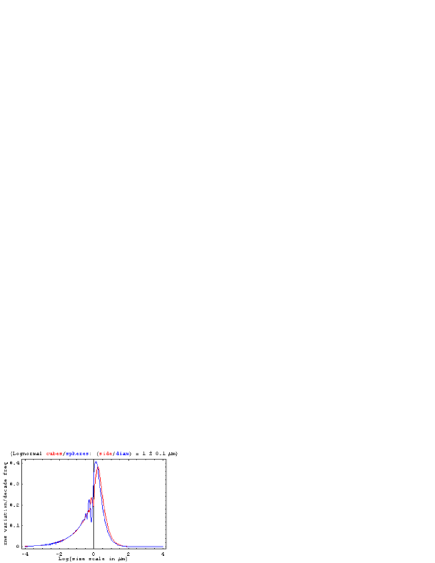
Figure 1: Root mean square compositional variability per decade of size-scale (or frequency) for log-normally distributed single-phase cubes one micron on a side, and spheres one micron in diameter.

Figure 2 illustrates the effect of changing grain size and standard deviation. Note that the effects of grain shape (e.g. Fourier ringing) are washed out as the range of sizes broadens. We also expect this to be the case as individual grain symmetries decrease. Of course, correlations in grain position or orientation might add new structure (e.g. lattice periodicities) to such heterogeneity spectra.

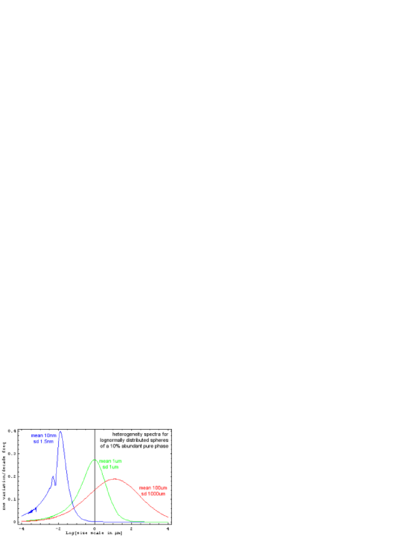
Figure 2: Root mean square compositional variability per decade of size-scale (or frequency) for log-normally distributed single-phase spheres with three different mean diameters and diameter standard deviations.

Our experience with fine-grained interplanetary dust particles (typical sizes $8\mu m$ in diameter) suggest that the porous or “re-entrant” material has a mean size for monomineralic grains (i.e. olivines, pyroxenes, sulfides) in the $0.1\mu m$ size rangeFraundorf (1981). However, particles with multi-micron sized monomineralic (e.g. olivine) grains with attached fine-grained material are also found. Thus for example a well-mixed lognormal grain size distribution with mean near $0.2\mu m$ but a much larger standard deviation may be appropriate for some types of interplanetary dust. The well-mixed model could be tested on microtomed dust particles not available at the time of the original paper, as well as against fine-grained carbonaceous meteorite matrices which may prove to be compositionally much coarser.

The tools described in this paper further allow one to model the relationship between individual dust particles and their “parent bodies”. For example, if the size and shape of individual grains is independent of composition, the correlation coefficient of a given particle to it’s source might be writtenFraundorf (1980)

$$\rho_{net}\cong\sum\limits_{i=1}^{m}{p_{i}\rho[\frac{D}{{d_{i}}}]}$$ (36)

Here $p_{i}$ is the volume fraction of grains of size $d_{i}$. More careful work on this question is likely worthwhile, particularly in anticipation of the Stardust comet sample return mission in 2006, at which time multiple particles from a single identified cometary source will become available.

Appendix B Log-log scale roughness spectroscopy

Here we turn from studies of compositional heterogeneity in three dimensions to the study of height variations across a surface in two dimensionsFraundorf and Armbruster (1993a, b). The transform equation (e.g. 3) in two dimensions is:

$$\gamma_{AB}[f]=2\pi\int\limits_{0}^{\infty}tJ_{0}[2\pi ft]{C_{AB}[t]dt},$$ (37)

where $J_{0}$ is the 0th order Bessel function of the first kind. As with the inverse in three dimensions (equation 4), the reverse transform in two dimensions is the forward transform, with $t$ and $f$ exchanged. The corresponding $t=0$ relationship in 2D then becomes:

$$C_{AB}[0]\equiv\int\limits_{0}^{\infty}2\pi{f}\gamma_{AB}df=\int\limits_{-\infty}^{\infty}{2\pi f^{2}}\gamma_{AB}d(\ln f).$$ (38)

Thus once again one might relate spectral density physically via a product (here $2\pi f^{2}\gamma_{AB}$) to that portion of the covariance $\sigma_{AB}[0]=C_{AB}[0]-\mu_{A}\mu_{B}$ between $A$ and $B$ in a given “e-fold” of frequency (or decade of frequency should one further multiply by $\ln 10$).

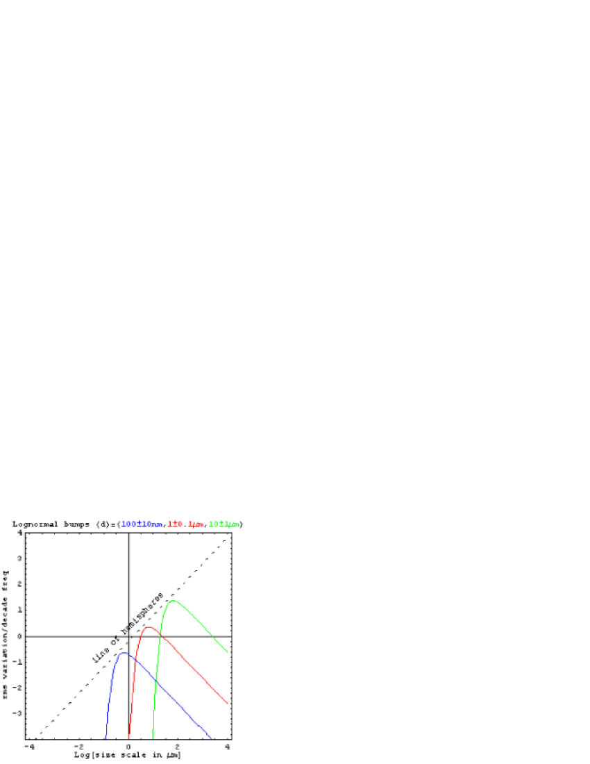
Figure 3: Root mean square roughness per decade of size-scale (or frequency) for log-normally distributed gaussian bumps three different mean diameters and diameter standard deviations.

Consider for example a Gaussian bump, of half-width $d$ at half of its maximum height $A$. If this bump is centered at the origin, it’s height as a function of position is $h[t]=A\exp[-\frac{t^{2}}{2d^{2}}]$. The 2D Fourier transform of this from 37 is $H[f]=2\pi d^{2}A\exp[-2\pi^{2}f^{2}d^{2}]$. Moving the bump from the origin will affect the transform’s phase, but not the spectral density obtained by squaring it’s amplitude: $\gamma_{hh}[f]=4\pi^{2}d^{4}A^{2}\exp[-4\pi^{2}f^{2}d^{2}]$. Inverse transforming this gives a height autocorrelation of $C_{hh}[t]=\pi d^{2}A^{2}\exp[-\frac{t^{2}}{4d^{2}}]$, which becomes the autocovariance $\sigma_{hh}[t]$ as well if indeed the spatial region integrated over is large enough to render the average height essentially zero.

Note in particular the “line of hemispheres” in Fig. 3. Crossing above this basically signals the existence of objects on a given width scale which are taller than they are wide. Grassy plains might represent an extreme in this regard. At the other extreme (exceptional flatness), silicon wafers immediately after growth of an epitaxial layer, with $0.13nm$ dimer row steps sometimes separated by a micron or more laterally represent the other extreme. We anticipate providing some experimental examples of these extremes, and further application examples, in a 2nd revision.

Appendix C Lattice fringe covariance fingerprints

In this appendix, covariances in high energy electron intensity as a function of scattering angle are examined as a tool for fingerprinting nanocrystal assemblagesFraundorf et al. (2004), given one or more high resolution lattice fringe images to work with. Calculations of these for some common nanoparticle structures are underway, and an expansion of this discussion is anticipated in a 2nd revision as well.