Resonant Spin Hall Conductance in Two-Dimensional Electron Systems with Rashba Interaction in a Perpendicular Magnetic Field

Abstract

We study transport properties of a two-dimensional electron system with Rashba spin-orbit coupling in a perpendicular magnetic field. The spin orbit coupling competes with Zeeman splitting to introduce additional degeneracies between different Landau levels at certain magnetic fields. This degeneracy, if occuring at the Fermi level, gives rise to a resonant spin Hall conductance, whose height is divergent as $1/T$ and whose weight is divergent as $-\ln T$ at low temperatures. The Hall conductance is unaffected by the Rashba coupling..

Remarkable phenomena have been observed in the two-dimensional electron gas (2DEG) over last two decades, including most notably, the discoveries of the integer and fractional quantum Hall effect Klitzing80 ; Tsui82 . From the point of view of applications, many semiconductor devices have been designed to take advantage of the properties of quantum physics. Nevertheless, a principal quantum aspect of an electron, its spin, has been largely ignored. In recent years, however, a new class of devices based on the spin degrees of freedom of electrons has emerged, giving rise to the field of spintronics.Prinz98Science ; Wolf01Science ; Awschalom02 Spintronics is believed to be a promising candidate for future information technology.Loss98 However, in order to be successful in device applications, effective spin injection into conventional semiconductors is essential. One proposal is to make use of the Rashba spin-orbit coupled 2DEGs to achieve this goal.Datta90 In particular, the spin-Hall effect predicted by Murakami et al Murakami03Science and Sinova et al Sinova03xxx has generated intensive theoretical studies. Thus far, all the studies have been limited to zero magnetic field.Shen03xxx

In this Letter, we study theoretically the spin transport properties of 2DEGs with a Rashba spin-orbit coupling in a perpendicular magnetic field. We find that the quantized charge Hall conductance remains intact in the presence of the Rashba spin-orbit coupling. However, a distinct spin Hall current can be generated. The spin Hall conductance can be made divergent or resonant by tuning the sample parameters and/or magnetic field $B$. The resonance effect stems from energy crossing of different Landau levels near the Fermi level due to the competition of Zeeman energy splitting and spin-orbit coupling. The height of the resonant peak in spin Hall conductance is proportional to $1/T$, and its weight is proportional to $-\ln T$ at low temperatures.

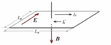
Figure 1: Illustration of the two dimensional electron system studied in the text.

We consider a two-dimensional electron system confined in the $x-y$ plane of an area $L_{x}\times L_{y}$ provided by a semiconductor quantum well as shown in Fig.1. The electron is subject to a spin-orbit interaction and to a perpendicular magnetic field $\vec{B}=-B\hat{z}$. An electric field is applied along the $y-$ axis. We are interested in the spin Hall conductance along the $x-$ direction. In our study, electron-electron interactions are neglected. The Hamiltonian for a single electron of spin-1/2 is given by

$$H = \frac{1}{2m}(\vec{p}+\frac{e\vec{A}}{c})^{2}+\frac{\lambda}{\hbar}\hat{z}\cdot(\vec{p}+\frac{e\vec{A}}{c})\times\vec{\sigma}$$ (1)

$$-\frac{1}{2}g_{s}\mu_{b}B\sigma_{z}+eEy,$$

where $m$, $-e$, $g_{s}$ are the electron’s effective mass, charge and Lande- $g$ factor, respectively. $\mu_{b}$ is the Bohr magneton, $\lambda$ is the Rashba coupling, and $\sigma_{\gamma}$ are the Pauli matrices. We choose the Landau gauge $\vec{A}=yB\hat{x}$, and consider periodic boundary condition in the $x$-direction, hence $p_{x}=k$ is a good quantum number.

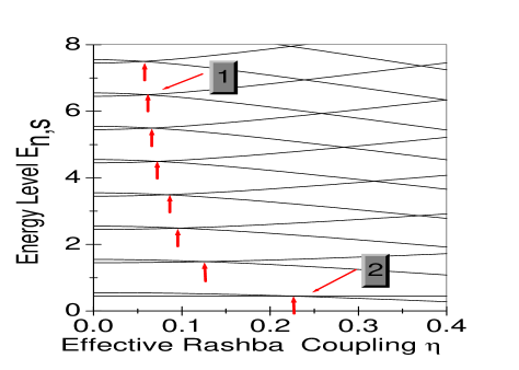
Figure 2: Landau levels of an electron as functions of $\eta=\lambda ml_{b}/\hbar^{2}$ for $g=g_{s}m/2m_{e}=0.1$. Arrows indicate those level crossings giving rise to resonant spin Hall conductance.

Let us start with a discussion of the single particle solution at $E=0$. The problem can be solved exactly. Rashba60 ; Luo88 ; Schliemann03 For a given k, the Hamiltonian can be written as,

$$H_{0}=\hbar\omega\{a_{k}^{{\dagger}}a_{k}+\frac{1-g\sigma_{z}}{2}+\sqrt{2}\eta(ia_{k}\sigma_{-}-ia_{k}^{{\dagger}}\sigma_{+})\},$$ (2)

where $\omega=eB/mc$, $\eta=\lambda ml_{b}/\hbar^{2}$, and $g=g_{s}m/2m_{e}$, with $m_{e}$ the mass of a free electron and $l_{b}=\sqrt{\hbar c/eB}$ the magnetic length. $a_{k}=[y+(k+ip_{y})c/eB]/\sqrt{2}l_{b}$, so that $[a_{k},a_{k}^{{\dagger}}]=1$. $\sigma_{\pm}=(\sigma_{x}\pm\sigma_{y})/2.$ The eigen energy of $H_{0}$ is given by

$$\epsilon_{ns}=\hbar\omega\left(n+\frac{s}{2}\sqrt{(1-g)^{2}+8n\eta^{2}}\right)\,,$$ (3)

with $s=\pm 1$, for $n\geq 1$; and $s=1$ for $n=0$. The eigenstate $\left|n,k,s\right\rangle$ has a degeneracy $N_{\phi}=L_{x}L_{y}eB/hc$, corresponding to $N_{\phi}$ quantum values of $k$. The two-component wavefunction is given by

$$\left|n,k,s\right\rangle=\left(\begin{array}[]{c}\cos{\theta_{ns}}\phi_{nk}\\ i\sin{\theta_{ns}}\phi_{n-1k}\end{array}\right)$$ (4)

where $\phi_{nk}$ is the eigenstate of the $n^{th}$ Landau level in the absence of the Rashba interaction. For $n=0,$ $\theta=0$, otherwise for $n\geq 1$, $\tan{\ \theta_{ns}}=u_{n}-s\sqrt{1+u_{n}^{2}}$, with $u_{n}=(1-g)/\sqrt{8n}\eta$. The energy levels as functions of dimensionless parameter $\eta$ are plotted in Fig. 2. An interesting feature of this system is the energy level crossing as $\eta$ changes by varying $B$ or $\lambda$. As we shall see below, this energy crossing, if it occurs at the Fermi level, gives rise to a resonance in the spin Hall conductance.

We now study the system in the presence of the $E$-field. The Hamiltonian $H$ can be rewritten as

$$H = H_{0}(E)+H^{\prime},$$

$$H^{\prime} = -(\eta el_{b}\sigma_{y}+kc/B)E,$$ (5)

where we have dropped an overall constant $-e^{2}E^{2}/2m\omega^{2}$. $H_{0}(E)$ is given by Eq. (2) of $H_{0}$ with the replacement of $y$ by $y+eE/m\omega^{2}$ in $a_{k}$. In the absence of Rashba coupling, $H$ is exactly solvable. For $\lambda\neq 0$ and $E\neq 0$, an exact solution of $H$ is not available. While $p_{x}$ remains to be a good quantum number, $H^{\prime}$ couples the state $\left|n,k,s\right\rangle$ with $\left|n\pm 1,k,s^{\prime}\right\rangle$. Below we shall calculate the charge and spin Hall current to the order of $O(E)$ by treating $H^{\prime}$ as a perturbation up to the first order. Our theory is accurate for the linear response. The charge current operator of a single electron is given by currentdef

$$j_{c} = -ev_{x},$$

$$v_{x} = [x,H]/\left(i\hbar\right)=p_{x}/m+y\omega+(\lambda/\hbar)\sigma_{y},$$ (6)

and the spin-$\gamma$ component current operator is

$$j_{s}^{\gamma}=\frac{\hbar}{2}(S^{\gamma}v_{x}+v_{x}S^{\gamma}).$$ (7)

Let $(j_{c,s})_{nks}$ be the current carried by an electron in the state $\left|n,k,s\right\rangle$ of $H$, including also the perturbative correction. We have, up to the first order in $E$,

$$(j_{c,s})_{nks}=(j_{c,s}^{(0)})_{nks}+(j_{c,s}^{(1)})_{nks},$$ (8)

where the superscript refers to the $0^{th}$ or $1^{st}$ order in the perturbation in $H^{\prime}$, and

$$(j_{c,s}^{(0)})_{nks} = \left\langle n,k,s\right|j_{c,s}\left|n,k,s\right\rangle,$$

$$(j_{c,s}^{(1)})_{nks} = \sum_{n^{\prime}s^{\prime}}\frac{\left\langle n^{\prime},k,s^{\prime}\right|H^{\prime}\left|n,k,s\right\rangle\left\langle n,k,s\right|j_{c,s}\left|n^{\prime},k,s^{\prime}\right\rangle}{(\epsilon_{ns}-\epsilon_{n^{\prime}s^{\prime}})}$$ (9)

$$+h.c..$$

In the above equation, $n^{\prime}=n\pm 1$ since the matrix element vanishes for other values of $n^{\prime}$. Note that $H_{0}(E)$ depends on $E$ so that the $0^{th}$ order in $H$ also contributes to the current. The average current density of the $N_{e}$-electron system is given by

$$I_{c,s}=\frac{1}{L_{y}}\sum_{nks}(j_{c,s})_{nks}f(\epsilon_{nks}),$$ (10)

where $f$ is the Fermi distribution function, and $N_{e}=\sum_{nks}f(\epsilon_{nks})$. The charge or spin Hall conductance is then given by $G_{c,s}=I_{c,s}/E$.

Figure 3: Left: Average spin $\left\langle\sigma_{z}\right\rangle$ (unit: $\hbar/2$) per electron as a function of $1/B$. Right: spin Hall conductance versus $B$ at $T=0$. The parameters used are $\lambda=0.9\times 10^{-11}eVm,$ $n_{e}=1.9\times 10^{16}/m^{2}$, $g_{s}=4$, and $m=0.05m_{e}$, taken for the inversion heterostructure In_0.53Ga_0.47As/In_0.52Al_0.48As. (See Ref.Nitta97prl ).

We first present the results for the charge current and the spin currents in the spin-$x$ and -$y$ components. They are found to be

$$(j_{c})_{nks} = (EL_{y})e^{2}/hN_{\phi},$$

$$(j_{s}^{x})_{nks} = 0,$$

$$(j_{s}^{y})_{nks} = \frac{\lambda}{2\hbar}\left(1+\frac{s}{\eta}\sqrt{\frac{n}{2(1+u_{n}^{2})}}\right)\,.$$ (11)

From the above expression, we obtain that the Hall conductance $G_{c}=\nu e^{2}/h$, with the filling factor $\nu=N_{e}/N_{\phi}$. In fact this result holds to all order in $E$. This is because the only k-dependence of the energy comes from the $-kcE/B$ term in $H$, thus the group velocity $v_{x}=cE/B$. This result is consistent with the quantization of the Hall conductance:Prange87 the spin-orbit coupling does not change the charge current carried by each state. The spin-$y$ component current is found to be finite even in the absence of $E$. Similar result was reported previously in the systems at $B=0$.Rashba03prb In the limit $B\rightarrow 0$, our result gives $I_{s}^{y}\rightarrow\lambda n_{e}/(2\hbar)$, which is the same as the result found at $B=0$. Since this is not a response to any external field, we will not give further discussion here.

The spin-z component current is the most interesting. Within the perturbation theory, $I_{s}^{z}$, hence $G_{s}^{z},$ can be divided into two parts. The part arising from the $0^{th}$ order in $H^{\prime}$ is found to be the product of the spin polarization $S^{z}$ and the Hall conductance $G_{c}$ divided by the electron charge ($-e$),

$$G_{s}^{z}{}^{(0)} = -\langle S^{z}\rangle(G_{c}/e),$$

$$\langle S^{z}\rangle = (\hbar/2\nu)\sum_{n,s}\cos{(2\theta_{ns})}f(\epsilon_{ns})$$ (12)

Since the charge current is a constant, $G_{s}^{z}{}^{(0)}\propto\langle S^{z}\rangle$. The spin polarization per electron at $T=0$ as a function of the Landau level filling is plotted in Fig. 3a, for a set of parameters appropriate for In_0.53Ga_0.47As/In _0.52Al_0.48As.Nitta97prl . $\langle S^{z}\rangle$ oscillates as a result of the alternative occupation of mostly spin-up and mostly spin-down electrons. It reaches maxima at filling $\nu=$ odd integers, and minima at $\nu=$ even integers at a strong field $B$. There is a jump at $B=B_{0}\approx 6.1T$ or $\nu=12.6$. Below the field, $\langle S^{z}\rangle$ reaches minima at filling $\nu=$even integers and minima at $\nu=$odd integer. The jump is caused by the energy crossing of two Landau levels with almost opposite spins. This value of the filling factor corresponds to the parameter $\eta$ at point $1$ in Fig.2. In the weak field limit, $\langle S^{z}\rangle\rightarrow-geB/4\pi c,$ and the spin susceptibility approaches to a constant, $d\langle S^{z}\rangle/dB=-ge/4\pi c.$

The second part in $G_{s}^{z}$ arises from $H^{\prime}$, and shows a resonance.

$$G_{s}^{z}{}^{(1)}=\frac{e\eta}{8\pi\sqrt{2}}\sum_{n,s,n^{\prime}=n+1,s^{\prime}}\frac{f(\epsilon_{ns})-f(\epsilon_{n^{\prime}s^{\prime}})}{(\epsilon_{ns}-\epsilon_{n^{\prime}s^{\prime}})}$$

$$\times\left(\sqrt{n}\sin 2\theta_{ns}\sin^{2}\theta_{n^{\prime}s^{\prime}}-\sqrt{n^{\prime}}\cos^{2}\theta_{ns}\sin 2\theta_{n^{\prime}s^{\prime}}\right)$$ (13)

Resonance occurs when two states are close to degeneracy. For reasonable values of the Rashba coupling, this will happen only for the pair of states $\left|n,s=1\right\rangle$ and $\left|n+1,s^{\prime}=-1\right\rangle.$ However, at $T=0,$ if $\left|n,s\right\rangle$ and $\left|n+1,s^{\prime}\right\rangle$ are both occupied or both unoccupied, the contributions to $G_{s}$ from this pair vanish. Therefore, only the states near the Fermi level are important in the sum in Eq. (13). If the two states at the Fermi energy become degenerate, $G_{s}^{z}$ becomes divergent. Therefore, there is a resonance in the spin Hall conductance. The resonant condition (in the clean limit) is given by

$$\sqrt{(1-g)^{2}+8n\eta^{2}}+\sqrt{(1-g)^{2}+8\left(n+1\right)\eta^{2}}=2,$$ (14)

where $n\leq\nu/2\leq n+1$. In a sample of given $n_{e}$, and $\lambda\neq 0$ and $1>g>0$, there is a resonant magnetic field $B_{0}$ for the resonance as the solution of Eq. (14). In Fig. 3b, we show the result of $G_{s}^{z}$ at $T=0$ as a function of $\nu$, or $1/B$. In addition to the oscillations similar to $\langle S^{z}\rangle$, there is a pronounced resonance at $B_{0}$ or at filling $\nu=12.6$. At this filling the $13^{th}$ Landau level is partially filled. From Fig. 3b, we also see that there are satellite peaks around the resonant field $B_{0}$. The resonance point coincides with the jump point for $\left\langle S^{z}\right\rangle.$ The spin Hall conductance becomes divergent while $\left\langle S^{z}\right\rangle$ has only a finite jump at the energy crossing point near the Fermi level.

In order to analyze this resonance further, we focus on the two relevant states and neglect all other states in the problem. For simplicity we consider the two states $\left|0,+1\right\rangle$ and $\left|1,-1\right\rangle$. The linear response of the two level problem to the electric field can be studied analytically. The singular part of the spin Hall conductance near the resonant point (point 2 in Fig. 2) is caused by the mixing of the two states, and is given by (for filling $\nu<1$),

$$G_{s}^{z}=-\frac{D\,f_{-}(1-f_{+})}{\left|b\right|}\left(1-\exp\left[-\frac{g\hbar\omega_{0}\left|b\right|}{(1+g)k_{B}T}\right]\right),$$ (15)

where $D=e\sqrt{2}\nu g/4\pi(1+g)$, $\omega_{0}$ is the value of $\omega$ at the resonant field $B_{0}$. The Fermi distribution $f_{\pm}=(\exp[\left(\pm g\hbar\omega_{0}\left|b\right|/2(1+g)-\mu\right)/k_{B}T]+1)^{-1}$, where $\mu$ is the chemical potential measured relative to the mid of the two levels, and $b=(B-B_{0})/B_{0}$. At low $T$, as $b\rightarrow 0$, $G_{s}^{z}\rightarrow-Dg(1+g)^{-1}\hbar\omega_{0}/kT$, and $\int G_{s}^{z}db\rightarrow-D\ln\left[\hbar\omega_{0}/k_{B}T\right]$. In Fig. 4, we show $G_{s}^{z}$ (including both singular and non-singular parts) as a function of $B$ at several temperatures. As we can see, both the height and the weight of the resonant peak increase as the temperature decreases.

The calculations reported in this paper have been performed on a 2DEG without potential disorder. Since the effects of disorder in systems with Rashba coupling and strong magnetic field is not well understood at this point, we will make only a few general comments here. We assume that, just as in the case without Rashba coupling, the presence of disorder gives rise to broadening of the Landau level and localization so that the extended states in a Landau levels are separated in energy from those in the next one by localized states. Inspection of the Rahsba Hamiltonian shows that Lauhglin’s gauge invariant argument still holds,Laughlin81 and each Landau level with its extended states completely filled contribute $e^{2}/h$ to the Hall conductance. Thus we conclude that identical quantum Hall effect is observed whether the Rashba coupling is present or not. For the spin Hall conductance, we further assume that there is only one extended state per Landau level as in the case of no Rashba coupling, and that the spin current is carried only by extended states. The resonance discussed above will then occur if the extended state of the band $\left|n,s\right\rangle$ and the $\left|n+1,s\prime\right\rangle$ band can become degenerate. In principle, such a degeneracy is disallowed due to level crossing avoidance. However, since potential disorder does not couple states of different spins, any coupling between these two states will have to arise from Landau level mixing effect of the disorder in the absence of Rashba coupling. Provided this is negligible, the crossing avoidance gap will also be negligible.

In summary, we have studied the transport properties of two dimensional electron gas with a Rashba spin-orbit coupling in a perpendicular magnetic field. The Rashba spin-orbit coupling competes with the Zeeman energy splitting to cause the energy level crossing. When the level crossing occurs near the Fermi level, the spin Hall conductance becomes divergent or resonant, while the charge Hall conductance remain intact.

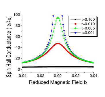
Figure 4: Spin Hall conductance as a function of $B$ at various temperatures for a two level system with $n_{e}$ fixed, $g=0.1,$ and $\nu=0.5$ at the resonant field $B_{0}$. $b=(B-B_{0})/B_{0},$ and $t=kT/\hbar\omega(B_{0})$.

This work was in part supported by RGC in Hong Kong (SQS), NFC (FCZ), and DOE/DE-FG02-04ER46124 (XCX).

References

- (1) K. v. Klitzing, G. Dorda, and M. Pepper, Phys. Rev. Lett. 45, 494 (1980).
- (2) D. C. Tsui, H. L. Stormer, and A. C. Gossard, Phys. Rev. Lett. 48, 1559 (1982).
- (3) G. A. Prinz, Science 282, 1660 (1998).
- (4) S. A. Wolf, D. D. Awschalom, R. A. Buhrman, J. M. Daughton, S. von Molnar, M. L. Roukes, A. Y. Chtchelkanova, and D. M. Treger, Science 294, 1488 (2001).
- (5) D. Awschalom, D. Loss, and N. Samarth (.eds), Semiconductor Spintronics and Quantum Computation (Springer, Berlin, 2002).
- (6) D. Loss and D. P. DiVincenzo, Phys. Rev. A 57, 120 (1998).
- (7) S. Datta and B. Das, Appli. Phys. Lett. 56, 665 (1990).
- (8) S. Murakami, N. Nagaosa, and S. C. Zhang, Science 301, 1348 (2003); cond-mat/0310005.
- (9) J. Sinova, D. Culcer, Q. Niu, N. A. Sinitsyn, T. Jungwirth, and A. H. MacDonald, to appear in Phys. Rev. Lett., (2004)/cond-mat/0307663; D. Culcer, J. Sinova, N. A. Sinitsyn, A. H. MacDonald, and Q. Niu, cond-mat/0309475.
- (10) S. Q. Shen, con-mat/0310368; A.A. Burkov and A.H. MacDonald, cond-mat/0311328; J. Schliemann and D. Loss, cond-mat/0310108; J. Hu, B.A. Bernevig, and C. Wu, cond-mat/0310093; L. Hu, J. Gao, and S. Q. Shen, cond-mat/0401231.
- (11) E. I. Rashba, Fiz. Tverd. Tela (Leningrad) 2, 1224 (1960) [Sov. Phys. Solid State 2, 1109 (1960)]; Y. A. Bychkov and E. I. Rashba, J. Phys. C 17, 6039 (1984).
- (12) J. Lou, H. Munekata, F. F. Fang, and P. J. Stiles, Phys. Rev. B 38, 10142 (1988); 41, 7685 (1990).
- (13) J. Schliemann, J. C. Egues, and D. Loss, Phys. Rev. B 67, 085302 (2003).
- (14) For brevity we write the current operators here in the Hilbert subspace .
- (15) R. E. Prange and S. M. Girvin (.eds), The Quantum Hall Effect, (Springer, Berlin, 1987).
- (16) E. I. Rashba, Phys. Rev. B 68, 241315 (2003).
- (17) J. Nitta, T. Akazaki, H. Takayanagi, and T. Enoki, Phys. Rev. Lett. 78, 1335 (1997).
- (18) R. B. Laughlin, Phys. Rev. B 23, 5632 (1981); B. I. Halperin, ibid. 25, 2185 (1982).