Message passing in random satisfiability problems

Abstract

This talk surveys the recent development of message passing procedures for solving constraint satisfaction problems. The cavity method from statistical physics provides a generalization of the belief propagation strategy that is able to deal with the clustering of solutions in these problems. It allows to derive analytic results on their phase diagrams, and offers a new algorithmic framework.

1 Message passing

Many NIPS participants can be confronted to the following type of generic problem [1]. A system involves many ’simple’ discrete variables, and each variable can take a certain number of discrete values (which is not too large). These variables interact, and the interactions can be written in the form of constraints, where each constraint involves a small fraction of all the variables. One wants to find the values of the variables which are compatible with all constraints (or, when this is impossible, find the values which minimize the number of violated constraints).

This ’constraint satisfaction problem’ (CSP) is a ubiquitous situation which shows up for instance in statistical physics, combinatorial optimization, error correcting codes, statistical inference,… It turns out that, in order to solve CSPs, these various disciplines have developed, often independently, some message passing procedures which turn out to be remarkably powerful. The general strategy involves two main steps:

• Organize the constraints and variables in a graph

• Exchange messages, of probabilistic nature, along the graph

We shall illustrate it here using as an example the famous ’satisfiability’ problem.

2 Satisfiability and complexity theory

The problem of satisfiability involves $N$ Boolean variables ${x_{i}\in\{0,1\}}$. There exist thus $2^{N}$ possible configurations of these variables. The constraints take the special form of ’clauses’, which are logical ’OR’ functions of the variables. For instance the clause $x_{1}\vee x_{27}\vee\bar{x}_{3}$ is satisfied whenever $x_{1}=1$ or $x_{27}=1$ or $x_{3}=0$. Therefore, among the $8$ possible configurations of $x_{1},x_{27},x_{3}$, the only one which is forbidden by this clause is $x_{1}=x_{27}=0$, $x_{3}=1$. An instance of the satisfiability problem is given by the list of all the clauses.

Satisfiability is a decision problem. One wants to give a yes/no answer to the question: is there a choice of the Boolean variables (called an ’assignment’) such that all constraints are satisfied (when there exists such a choice the corresponding instance is said to be ’SAT’, otherwise it is ’UNSAT’)?

This problem appears in many fields and its importance is a consequence of its genericity: an instance of the SAT problem can be seen as a logical formula (such as $(x_{1}\vee x_{27}\vee\bar{x}_{3})\wedge(\bar{x}_{11}\vee x_{2})\wedge\ldots$), and it turns out that any formula can be written in this form of the ’and’ function of several clauses, called ’conjunctive normal form’.

Satisfiability plays an essential role in the theory of computational complexity,because it was the first problem which has been shown to be ’NP-complete’, in a beautiful theorem by Cook in 1971 [2]. The NP problems are those decision problems where a ’yes’ answer can be checked in a time which is polynomial in $N$. This is a vast class of problems which contains such difficult problems as the traveling salesman, the problem of finding a Hamiltonian path in a graph (a path which goes once through all vertices), the protein folding problem, or the spin glass problem in statistical physics. The fact that satisfiability is NP-complete means that any other NP problem can be mapped to satisfiability in polynomial time. So if we happened to have a polynomial algorithm for satisfiability (i.e. an algorithm that solves the decision problem in a time which grows like a power of $N$), all the problems in NP would also be solved in polynomial time. This is generally considered unlikely, but the corresponding mathematical problem (whether the NP class is distinct or not from the ’P’ class of problems which are solvable in polynomial time) is an important open problem.

The result of Cook is a worst case analysis of the satisfiability problem. However it is known experimentally that many instances of this problem are easy to solve, and researchers have started to study some classes of instances in order to characterize the ’typical case’ complexity of satisfiability problems. A class of instances is a probability measure on the space of instances. A much studied problem in this framework is the random ’3-SAT’ problem. Each clause contains exactly three variables; they are chosen randomly in $\{x_{1},..,x_{N}\}$ with uniform measure, and each variable is negated randomly with probability $1/2$. This problem is particularly interesting because its difficulty can be tuned by varying one single control parameter, the ratio $\alpha=\frac{M}{N}$ of constraints per variable. One expects intuitively that for small $\alpha$ most instances are SAT, while for large $\alpha$ most of them are UNSAT. Numerical experiments have confirmed this scenario, but they indicate actually a more interesting behavior. The probability that an instance is SAT exhibits a sharp crossover, from a value close to $1$ to a value close to 0, at a threshold $\alpha_{c}$ which is around $4.3$. When the number of variables $N$ increases, the crossover becomes sharper and sharper [3, 4]. It has been shown that it becomes a staircase behavior at large $N$ [5]: almost all instances are SAT for $\alpha<\alpha_{c}$, almost all instances are UNSAT for $\alpha>\alpha_{c}$, and some bounds on the value of $\alpha_{c}$ have been derived[6, 7]. This threshold behavior is nothing but a phase transition as one finds in physics, and has been analyzed using the methods of statistical physics [3, 8].

A very interesting observation is that the algorithmic difficulty of the problem, measured by the time taken by the algorithm to answer if a typical instance is satisfiable, also depends strongly on $\alpha$: the typical problem is easy when $\alpha$ is well below or well above $\alpha_{c}$, and is much harder when $\alpha$ is close to $\alpha_{c}$. Therefore the region of phase transition is also the region which is interesting from the computational point of view.

3 Statistical physics of the random 3-SAT problem

In the last two decades, it has been realized that some concepts and methods developed in statistical physics can be useful to study optimization problems [9]. The interest in this type of approach has been focusing in recent years on the random satisfiability problem, following the works of colleagues like Kirkpatrick, Monasson and Zecchina [8, 10, 11]. This is indeed a choice problem for a multidisciplinary study, because the SAT-UNSAT transition is a phase transition in the usual statistical physics sense, and the algorithmic complexity of the problem shows up precisely in the neighborhood of this phase transition. On the analytical side, the first breakthrough used the replica method and computed some approximations of the phase diagram using either a ’replica symmetric’ approximation, or some variational approximation to the replica symmetry breaking solution. Hereafter I will mainly review the most recent developments initiated in [12, 13]. These have provided some analytical insight into the phase diagram of the problem, which turns out to be more complicated than originally thought, as well as a new algorithmic strategy based on message passing for the case of random 3-satisfiability.

The main analytical result on the phase diagram is summarized in Fig. 1. When one varies the control parameter $\alpha$ (the number of constraints per variable), there actually exist three distinct phases, separated by two thresholds $\alpha_{d}$ and $\alpha_{c}$. The threshold at $\alpha_{c}=4.267$ is the satisfiability threshold which separates the SAT phases at $\alpha<\alpha_{c}$ from the UNSAT phase at $\alpha>\alpha_{c}$. But in the SAT region,there actually exist two distinct phases. They differ by the structure of the space of SAT assignments (the ’SAT space’). For $\alpha<\alpha_{d}\simeq 3.86$, the set of SAT assignments builds one cluster which is basically connected [11, 14]. Starting from a generic SAT assignment (which is a point on the unit N-dimensional hypercube), one can step to another one nearby by flipping a finite number of variables. It turns out that one can get from any generic SAT assignment to any other one through a sequence of such steps, always staying in the SAT space. On the other hand, for $\alpha>\alpha_{d}$, this SAT space becomes disconnected: the SAT assignments are grouped into many clusters. It is impossible to get from one cluster to another one without having to flip at some moment a macroscopic fraction of the variables. Simultaneously, the space of configurations develops many ’metastable states’: imagine walking along the configuration space (the N-dimensional hypercube), flipping one variable at a time, but allowing only the moves which decrease, or leave constant, the number of violated clauses. Such an algorithm will get trapped into some ’metastable clusters’, which are connected clusters of assignments, all violating the same (non-zero) number of clauses. This structure has some direct algorithmic implication: the separation of clusters in the phase $\alpha>\alpha_{d}$ makes it very difficult for algorithms based on local moves to find a SAT assignment. The phase $\alpha<\alpha_{d}$ is thus called the ’Easy-SAT’ phase, while the one between $\alpha_{d}$ and $\alpha_{c}$ is the ’Hard-SAT’ phase.

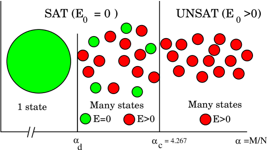
Figure 1: The phase diagram of the random 3-SAT problem: when one increases the ratio $\alpha$ of constraints to variables, one finds successively an Easy-SAT phase, a Hard-SAT phase, and an UNSAT phase

These results have been obtained using the cavity method. Originally this method was invented in the study of spin glass theory, in order to solve the Sherrington Kirkpatrick model [15]. It is only recently that new developments in this method allowed to solve ’finite connectivity’ problems where each variable interacts with a small number of other variables[16]. Thanks to these development, it has become possible to study constraint satisfaction problems. Although the method is not fully rigorous, the self-consistency of the main underlying hypothesis has been checked [17, 18, 19], and therefore the results concerning the satisfiability threshold, as well as crucial features of the phase diagram like the existence of the intermediate Hard-SAT phase, are conjectured to be exact results, not approximations. Of course, it is very important to develop rigorous mathematical approaches in order to confirm or infirm them.

It turns out that the cavity method when applied to one given instance of the problem amounts to a message passing procedure which can also be used as an algorithm. Therefore one surprising offspring of the theoretical development of the cavity method in recent years, which aimed at answering very fundamental questions concerning the phase diagram, has been the finding of a new class of algorithms, which turn out to be very efficient in the Easy-SAT phase.

The next sections aim at describing the main ideas of the cavity method, taking the point of view of the message passing algorithm. It is impossible to explain all the details, or to give the justification, for all these steps. The interested reader is referred to refs [16] for the basic concepts of the cavity method in finite connectivity disordered systems, and to refs [12, 13, 20, 18] for the solution of the random satisfiability problem.

4 Factor graphs and warning propagation

The first step consists in a graphical representation of the satisfiability problem. Each clause is represented by a function node, connected to the various variables which appear in the clause, as described in Fig.2.

Figure 2: Factor graph representation of satisfiability: A variable is represented by a circle. A clause is represented by a square, connected with a full (resp. dashed) line to a variable when this variable appears as such (resp. negated) in the clause. Left hand side: The clause $\bar{x}_{1}\vee x_{2}\vee\bar{x}_{3}$. Right hand side: the factor graph representing the formula: ${(\bar{x}_{1}\vee\bar{x}_{2}\vee\bar{x}_{4})}{\wedge}{(x_{1}\vee\bar{x}_{2})}{\wedge}{(x_{2}\vee x_{4}\vee x_{5})}{\wedge}{(x_{1}\vee x_{2}\vee\bar{x}_{5})}{\wedge}{(x_{1}\vee\bar{x}_{3}\vee x_{5})}$

Factor graphs turn out to be very useful in various contexts, including statistical inference [21] and error correcting codes [22]. The general formalism is described in [23].

In a random 3-SAT problem with $N$ variables and $M=\alpha N$ clauses, in the large $N$ limit, it is easy to see that the factor graph is a random bipartite graph, where the function nodes have a fixed connectivity equal to 3, and the variable nodes have a Poisson distributed connectivity with a mean $3\alpha$.

The simplest case of message passing is the warning propagation. Along all the edges of the graph, one passes messages. If clause $a$ involves variable $i$, the message $u_{a\to i}\in\{0,1\}$ sent from clause $a$ to variable $i$ is a way for clause $a$ to inform variable $i$: A warning $u_{a\to i}=1$ means : “According to the messages I have received (from the other variables which are connected to me), you should take the value which satisfies me!”. When $u_{a\to i}=0$, this means that no warning is passed, which means a message saying: “According to the messages I have received, there is no problem, you can take any value!”

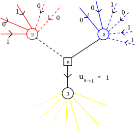
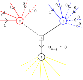
Figure 3: Two examples of warning propagation in a clause $a$. In order to determine the message which it passes to variable $1$, clause $a$ considers all the messages received by the other variables to which it is connected, here the variables $2$ and $3$. On the left hand side, the messages received by $2$ tell it to take the value $x_{2}=1$, which does not satisfy clause $a$, and the messages received by $3$ tell it to take the value $x_{3}=0$, which does not satisfy clause $a$. Therefore, in order to be satisfied, clause $a$ must rely on variable $1$. It thus sends a warning $u_{a\to 1}=1$. Right hand side: an example where no warning is sent, because variable $3$ is told by its environment to take the value $x_{3}=1$, which satisfies clause $a$.

It can be shown that warning propagation converges and gives the correct answer in a satisfiability problem described by a tree factor graph (such a problem can be nontrivial if there are, among the clauses, some ’unit clauses’, involving a single variable, and forcing this variable): the problem is SAT if and only if, on each variable node, there are no contradictory messages.

This simple warning propagation corresponds to some limiting case of the celebrated belief propagation (“BP”) algorithm. The basic idea of BP is to study the probability space of all SAT assignments with uniform measure. Consider again the clause in Fig.3. Imagine one knows the joint ’cavity’ probability $P^{(a)}(x_{2},x_{3})$ for the variables $x_{2},x_{3}$ when the clause $a$ is absent. Then one can deduce the following estimate from $a$ concerning the state of $1$:

$$P_{a\to 1}(x_{1})=\sum_{x_{2},x_{3}}C_{a}(x_{1},x_{2},x_{3})P^{(a)}(x_{2},x_{3})\ ,$$ (1)

where $C_{a}$ is the indicator function of clause $a$, equal to one if and only if the clause is satisfied. The probability distribution of $x_{1}$ in the absence of a clause $b$ is given by:

$$P^{(b)}(x_{1})=C\prod_{a\in V(1)\setminus b}P_{a\to 1}(x_{1})$$ (2)

where $C$ is a normalization constant.

These exact equations are useless as such, but they become very useful if one adds the hypothesis that

$$P^{(a)}(x_{2},x_{3})\sim P^{(a)}(x_{2})P^{(a)}(x_{3})\ .$$ (3)

Then eqs (1,2) close onto a set of self-consistent equations for the cavity probabilities $P^{(a)}(x)$. These equations can be interpreted as a message passing procedure which is the BP algorithm; they also carry the name of Bethe approximation in statistical physics. The warning propagation equations are some version of BP in which one focuses onto the variables which are forced to take one given value in all the SAT configurations (in the statistical physics approach they correspond to writing the Bethe equations directly at zero temperature). The onset of clustering at this zero temperature level signals the existence of clusters in which a given variable is frozen (it takes the same value in all configurations of the cluster): it takes place at a value $\alpha\sim 3.91$.

The main question is whether the factorization approximation (3) is correct. If the factor graph is a tree, it is obviously correct. In the case of a random 3-SAT, or random K-SAT problem, one may notice that generically the factor graph is locally tree-like: the loops appear only at large distances (of order $\log N$). Therefore, in the absence of clause $a$, the two variables $x_{2},x_{3}$ are far apart. In such a situation one may hope that the factorization will hold, in the large $N$ limit. However this is true only in the case where there is a single pure state in the system (i.e. a single cluster of solutions). If there are several pure states, it is well known in statistical physics that the correlations of the variables decay at large distances only when the probability measure is restricted to one pure state.

5 Proliferation of states: survey propagation

Therefore one can expects the BP, or the warning propagation, to be correct in the Easy-SAT phase. In the Hard-SAT phase where pure states proliferate, the BP would be correct if we had a way to restrict the measure to the SAT configurations in one given cluster. However there is no way to achieve this globally. BP is a local message passing procedure. Locally it will tend to find equilibrated configurations corresponding to one cluster, but there is no way to select the same cluster in distant parts of the factor graph.

In order to handle such a situation the cavity method introduces generalized messages: Along each edge $a-i$, a message is sent from clause $a$ to variable $i$. This message is a survey of the elementary messages in the various clusters of SAT configurations. Because warnings are so simple (this is where it is useful to use warnings rather than standard BP), the survey is characterized by a single real number $\eta_{a\to i}$, which gives the probability of a warning being sent from constraint $a$ to variable $i$, when a cluster is picked up at random in the set of all clusters of SAT assignments.

The survey propagation (SP) equations are easily written. Looking again at the clause of Fig.3, let us denote by $U$ the set of function nodes, distinct from $a$, connected through a full line to variable $x_{2}$, and $V$ the set connected through a dashed line. Introduce the probabilities that no warnings are sent from $U$ and $V$, given by $\pi^{2}_{+}=\prod_{b\in U}(1-\eta_{b\to 2})$ and $\pi^{2}_{-}=\prod_{b\in V}(1-\eta_{b\to 2})$. Similar quantities $\pi^{3}_{\pm}$ are introduced for the variable $x_{3}$. Then the SP equations read:

$$\eta_{a\to 1}=\frac{\pi^{2}_{-}(1-\pi^{2}_{+})}{\pi^{2}_{+}+\pi^{2}_{-}-\pi^{2}_{+}\pi^{2}_{-}}\ \ \frac{\pi^{3}_{+}(1-\pi^{3}_{-})}{\pi^{3}_{+}+\pi^{3}_{-}-\pi^{3}_{+}\pi^{3}_{-}}$$ (4)

It turns out that the propagation of these surveys along the graph converges for a generic problem in the whole Hard-SAT phase.

These SP equations can be used in two ways. When iterated on one given sample, they provide very interesting information concerning each variable: From the set of surveys, one can compute for instance the probability that one variable is constrained to $0$, when one chooses a SAT cluster randomly. The survey inspired decimation algorithm [12, 13] uses this information as follows: it identifies the most biased variable (the one which is polarized to 1, or to 0, with the largest probability), and fixes it. Then the problem is reduced to a new satisfiability problem with one variable less. One can run again the SP algorithm on this smaller problem and iterate the procedure. This simple strategy finds SAT assignment in the region $\alpha<4.252$ (quite close to the UNSAT threshold $\alpha_{c}=4.267$), in a time of order $N\log N$ which allows to reach large sample sizes of a few million variables. Some backtracking in the way one performs the decimation [24] allows to get closer to the threshold, but until now it is not known if these survey based algorithms will allow to solve the algorithmic problem in the whole Hard-SAT phase or not.

On the other hand one can also use the SP equations in order to find analytical results. The idea is to perform a statistical analysis of the SP equations: one introduces the probability density $P(\eta)$, when one picks up an edge $a-i$ randomly in a large random 3-SAT problem, that the survey $\eta_{a\to i}$ takes a given value $\eta$. The SP equations (4) allow to write a self-consistent non-linear integral equation for $P(\eta)$. Solving these equations, one can deduce all the features of the phase diagram of Fig.1. The thresholds found for random K-sat, for $K=3,4,5,6,10$, are respectively equal to $4.267,\;9.931,\;21.12,\;43.37,\;708.9$ (see [18]).

The equations can also be generalized to study the UNSAT phase, in which one can determine the minimal number of violated clauses, both analytically, and also algorithmically on one given sample, but this goes beyond the present paper.

This general cavity method strategy can also be used in other constraint satisfaction problems [25], and has found non-trivial results for instance on the coloring problem[26]. A particularly interesting case is the XOR-SAT problem [27], where the same type of phase diagram is found, and the cavity method result can be checked versus rigorous computations. It is also worth mentioning that for $K$ even, the SAT-UNSAT threshold $\alpha_{c}$ found with the cavity method has been shown to be an upper bound to the correct result[28]. Our conjecture is that this bound is actually tight.

To summarize, we have considered sparse network of many interacting elements, with interactions taking the form of constraints on their relative values. In this situation, one often finds a “Hard-SAT” phase, with an exponential number of well separated solution clusters, together with an exponentially larger number of ’metastable states’. It turns out that the local exchange of probabilistic messages between the elements provides a very detailed statistical information on the various solutions. One can expect that this general framework will also find applications in neural network studies.

Acknowledgments

The results presented here have been obtained in various collaborations, mainly with G. Parisi and R. Zecchina, and also with A. Braunstein, S. Mertens, M. Weigt.

References

- [1] M. Mézard, Science 301 (2003) 1685.
- [2] S. Cook, Proc. 3rd Ann. ACM Symp. on Theory of Computing, Assoc. Comput. Mach., New York, 1971, p. 151.
- [3] S. Kirkpatrick, B. Selman, Science 264, 1297 (1994).
- [4] J.A. Crawford and L.D. Auton, Artif. Intell. 81, 31-57 (1996).
- [5] E. Friedgut, J. Amer. Math. Soc. 12 (1999) 1017.
- [6] O. Dubois, Y. Boufkhad and J. Mandler, Proc. 11th ACM-SIAM Symp. on Discrete Algorithms, 124 (San Francisco, CA, 2000).
- [7] D. Achlioptas and C. Moore, http://arXiv.org/abs/cond-mat/0310227; D. Achlioptas and Y. Peres, http://arXiv.org/abs/cs.CC/0305009.
- [8] R. Monasson, R. Zecchina, S. Kirkpatrick, B. Selman and L. Troyansky, Nature (London) 400, 133 (1999).
- [9] O. Dubois, R. Monasson, B. Selman and R. Zecchina (Eds.), Theoret. Comp. Sci. 265 (2001).
- [10] R. Monasson and R. Zecchina, Phys. Rev. E 56 1357–1361 (1997).
- [11] G. Biroli, R. Monasson and M. Weigt, Euro. Phys. J. B 14 551 (2000).
- [12] M. Mézard, G. Parisi and R. Zecchina, Science 297, 812 (2002) (Sciencexpress published on-line 27-June-2002; 10.1126/science.1073287).
- [13] M. Mézard and R. Zecchina, Phys.Rev. E 66 (2002) 056126.
- [14] G. Parisi, cs.CC0301015.
- [15] M. Mézard, G. Parisi and M.A. Virasoro, Spin Glass Theory and Beyond, World Scientific, Singapore (1987).
- [16] M. Mézard, and G. Parisi, Eur.Phys. J. B 20, 217–233 (2001). M. Mézard and G. Parisi, J. Stat. Phys. 111 (2003) 1.
- [17] A. Montanari and F. Ricci-Tersenghi, Eur. Phys. J. B33 (2003) 339.
- [18] S. Mertens, M. Mézard and R. Zecchina, http://arXiv.org/abs/cs.CC/0309020.
- [19] A. Montanari, G. Parisi and F. Ricci-Tersenghi, http://arXiv.org/abs/cond-mat/0308147.
- [20] A. Braunstein, M. Mézard, R. Zecchina, http://fr.arXiv.org/abs/cs.CC/0212002.
- [21] J. Pearl, Probabilistic Reasoning in Intelligent Systems, 2nd ed. (San Francisco, MorganKaufmann,1988).
- [22] Special issue on Codes, Graphs and Iterative Algorithms, IEEE Trans. Info. Theory vol.47, no2 (2001).
- [23] F.R. Kschischang, B.J. Frey and H.-A. Loeliger, IEEE Trans. Info. Theory 47 (2001) 498.
- [24] G. Parisi, cond-mat/0308510.
- [25] A. Braunstein, M. Mézard, M. Weigt and R. Zecchina, cond-mat/0212451.
- [26] R. Mulet, A. Pagnani, M. Weigt, R. Zecchina, Phys. Rev. Lett. 89 (2002)268701.
- [27] M. Mézard, F. Ricci-Tersenghi, R. Zecchina, J.Stat. Phys 111 (2003) 505. S. Cocco, O. Dubois, J. Mandler, R. Monasson, http://arXiv.org/abs/cond-mat/0206239.
- [28] S. Franz and M. Leone, http://arXiv.org/abs/cond-mat/0208280.