The Generic, Incommensurate Transition in the two-dimensional Boson Hubbard Model

Abstract

The generic transition in the boson Hubbard model, occurring at an incommensurate chemical potential, is studied in the link-current representation using the recently developed directed geometrical worm algorithm. We find clear evidence for a multi-peak structure in the energy distribution for finite lattices, usually indicative of a first order phase transition. However, this multi-peak structure is shown to disappear in the thermodynamic limit revealing that the true phase transition is second order. These findings cast doubts over the conclusion drawn in a number of previous works considering the relevance of disorder at this transition.

I Introduction

Quantum phase transitions occurring in bosonic systems have experienced a surge of interest lately, due to recent experiments showing clear evidence for a quantum phase transition occurring in an optical lattice Greiner et al. (2002). In these experiments, one-, two- and three-dimensional lattice structures are imposed on the bosonic system by using lasers to create standing wave patterns. The lattice parameters and the lattice structure of this artificial lattice can therefore be experimentally tuned, creating an almost ideal setting for studying quantum phase transitions occurring in bosonic systems. Here we shall mainly be concerned with the case of a two-dimensional system. In the simplest setting the quantum phase transition is in this case believed to occur between a Mott insulating (MI) phase where the number of bosons per site is fixed and the phase therefore incompressible and a superfluid (SF) phase where the bosons freely hop throughout the lattice. However, several other phases are also possible Kuklov et al. (2003).

In the experiments described above the constituent atoms are clearly bosons and quantum phase transitions observed in ⁴He films Crowell and Reppy (1993) should be in the same superfluid-insulator (SF-I) universality class. A detailed scaling theory of the SF-I phase transition arising in two-dimensions as described by the bosonic version of the Hubbard model was developed in a seminal paper by Fisher et. al Fisher et al. (1989), in particular the transition in the presence of disorder was investigated and it was pointed out that for the SF-I transition in a disordered systems the insulating phase would in almost all situations not be a Mott insulator but instead a compressible Bose glass. Subsequent work showed that the same physics should apply also to quantum phase transitions occurring in superconducting systems dominated by a diverging phase coherence length Fisher et al. (1990); Fisher (1990) making the fermionic degrees of freedom irrelevant at the critical point. The reasoning being that, at the scale of the diverging phase coherence length the size of the individual Cooper pairs would be negligible and the underlying physics should therefore be dominated by the bosonic degrees of freedom. The scaling theory for the SF-I transition Fisher et al. (1989), mainly focusing on phase fluctuations, should therefore also apply to the two-dimensional superconductor-insulator (SC-I) transition. Ensuing experiments showed support for this scaling picture arising in superconducting films Liu et al. (1993); Marković et al. (1998, 1999) and several similar systems such as Josephson Junction arrays Zant et al. (1992). This scaling theory predicts that in two dimensions the quantum phase transitions for both the SF-I as well as the SC-I transition should take place directly from the superfluid or superconducting phase into the insulating phase with no intervening metallic phase. However, more recent experiments Mason and Kapitulnik (1999) and theoretical studies Wagenblast et al. (1997); Dalidovich and Phillips (2001); Das and Doniach (1999); Phillips and Dalidovich (2003) have pointed to the possibility of a metallic phase occurring in two-dimensional bosonic systems in particular in the presence of dissipation Wagenblast et al. (1997); Dalidovich and Phillips (2001).

Only at very special points does the SF-I occur at a commensurate filling factor. At these points the scaling theory of Fisher et al. Fisher et al. (1989) predicts that the transition is in the $d+1$ dimensional $XY$ class dominated by phase-fluctuations. More often the transition occurs at an incommensurate chemical potential which is in a different universality class. This more generic transition is expected to be mean-field like Fisher et al. (1989) and is the focus of the present paper.

Initial quantum Monte Carlo (QMC) simulations Krauth and Trivedi (1991); Krauth et al. (1991); Zhang et al. (1995) performed directly on the boson Hubbard model showed clear evidence for a direct SF-I transition. These simulations were constrained to systems with a fixed particle number and therefore always incompressible. Implicitly only the commensurate transition was studied. Subsequent studies Sørensen et al. (1992); Wallin et al. (1994) exploiting a mapping to the link-current model removing this constraint focused on the phase transition in the presence of strong disorder and showed clear evidence for a transition from the superfluid to a Bose glass phase, as did studies at fixed densities Krauth et al. (1991).

A point of controversy has been the phase transition occurring at weak disorder. A generalization Chayes et al. (1986) of the Harris criterion shows that the transition is stable towards disorder if $\nu\geq 2/d$. In $d=2$ the $d+1$ dimensional $XY$ does presumably not satisfy this inequality and neither does the mean-field $\nu=1/2$ predicted to occur at the generic transition. The scaling theory Fisher et al. (1989) therefore predicts that in all cases the Bose-glass phase intervenes between the superfluid and insulating phases. This prediction was however contradicted by numerical simulations showing evidence for a direct SF-I transition at a commensurate chemical potential in the presence of weak disorder Kisker and Rieger (1997). Furthermore, Lee et al. Park et al. (1999); Lee et al. (2001, 2002) reported evidence for a direct SF-I transition also at incommensurate chemical potentials. From these studies one would conclude that the SF-I transition should be stable towards the introduction of disorder, contradicting the scaling theory.

The recent development of worm algorithms Prokof’ev and Svistunov (2001); Alet and Sørensen (2003a) have allowed for the study of significantly larger system sizes and Prokof’ev and Svistunov Prokof’ev and Svistunov (2004, 2003) have shown evidence for the relevance of disorder at the transition occurring at commensurate chemical potentials with the universal behavior only setting in at very large system sizes. The existence of a multicritical line proposed in Ref. Lee et al., 2001, 2002 was also ruled out by these studies. However, the controversy surrounding the incommensurate case still remains. In fact, to our knowledge, no strong numerical evidence exists supporting the evidence of mean-field like exponents even in the absence of disorder for the generic transition, the results implicit in previous studies of the transition in the presence of disorder Park et al. (1999); Lee et al. (2001, 2002) as well as studies considering longer range interactions and the possibility of supersolid phases v. Otterlo and Wagenblast (1994); v. Otterlo et al. (1995) being limited to restrictively small lattice sizes. The results including longer range interactions were subsequently criticized Batrouni et al. (1995). All these studies Kisker and Rieger (1997); v. Otterlo and Wagenblast (1994); v. Otterlo et al. (1995); Park et al. (1999); Lee et al. (2001, 2002); Prokof’ev and Svistunov (2004, 2003) were performed using the link-current representation which we shall also use in this study.

In light of this wealth of experimental and theoretical studies it is perhaps surprising that fundamental aspects of the SF-I transition as it occurs at an incommensurate chemical potential are still controversial. This so called generic transition is the one most likely to describe real experiments and in the present paper we present large-scale numerical results using a recently developed geometrical worm algorithm, capable of yielding precise results for lattice sizes largely surpassing previous studies, thereby allowing us to shed new light on this transition. In particular we show that, due to the fact that this transition is dominated by fluctuations of the particle number, simulations on finite lattice will in most cases show clearly defined peaks in the energy histograms reminiscent of a first-order transition. Only in the thermodynamic limit do the peaks coalesce and a second-order transition is recovered. As stressed by Prokof’ev and Svistunov Prokof’ev and Svistunov (2004, 2003) for the commensurate transition, extreme care should therefore be taken when applying a finite-size scaling analysis. For the relative small lattice sizes used in the studies by Lee et al. Lee et al. (2001, 2002) the true influence of disorder is therefore likely even further obscured by these finite-size energy gaps associated with the first-order transition.

In the remainder of this section we discuss the Boson Hubbard model and the particular link-current representation that we use for this study as well as the associated phase-diagram. Section II describes the numerical techniques employed and Section III focuses on our results showing features characteristic of a first-order transition for finite lattices, which are found to disappear in the thermodynamic limit. We conclude with a discussion in Section IV.

I.1 The model

The simplest model we can write down for interacting bosons must at least include an on-site repulsion term $U$ as well as a competing hopping term parametrized by the hopping strength $t$. In the absence of the on-site repulsion term a bosonic system would always condense and would always be superfluid at $T=0$. Since we in the present paper in particular focus on the generic transition occurring at an incommensurate filling we also include a chemical potential, $\mu$. We thus arrive at the well known boson Hubbard model:

$$H_{\rm bH}=\sum_{\bf r}\left(\frac{U}{2}\hat{n}_{\bf r}(\hat{n}_{\bf r}-1)-\mu\hat{n}_{\bf r}\right)-\frac{t}{2}\sum_{\langle{\bf r},{\bf r^{\prime}}\rangle}(\hat{\Phi}^{\dagger}_{\bf r}\hat{\Phi}_{\bf r^{\prime}}+c.c)\ .$$ (1)

Here $\Phi^{\dagger}_{\bf r}$ ($\Phi_{\bf r}$) is the creation (annihilation) operator at site ${\bf r}$ and $\hat{n}_{\bf r}=\hat{\Phi}^{\dagger}_{\bf r}\hat{\Phi}_{\bf r}$ is the number operator. At $t=0$ the bosons are completely localized in Mott insulating phases while it can be shown Fisher et al. (1989) that a non-zero $t$ eventually gives rise to a superfluid phase with the Mott insulating phase persisting in a series of lobes into the superfluid. In the MI phase the particle number is fixed and only at the tip of the MI lobes does the density not change at the SF-I transition. This transition is therefore dominated by phase-fluctuations and is in the $d+1$-dimensional $XY$ class. The generic transition, occurring at incommensurate filling factors, is however dominated by fluctuations in the particle number and is expected to be characterized by mean-field exponents Fisher et al. (1989).

We can simplify the Hamiltonian Eq. (1) by integrating out amplitude fluctuations. We first set $\hat{\Phi}_{\bf r}\equiv|\hat{\Phi}_{\bf r}|e^{i\hat{\theta}_{\bf r}}$, where $\theta_{\bf r}$ is the phase of a quantum rotor. By performing the integration Sørensen et al. (1992); Wallin et al. (1994) $H_{\rm bH}$ then becomes equivalent to the (N=2) model of quantum rotors $(\cos(\theta_{\bf r}),\sin(\theta_{\bf r}))$, that describes a wide range of phase transitions dominated by phase-fluctuations:

$$H_{\text{qr}}=\frac{U}{2}\sum_{\bf r}\left(\frac{1}{i}\frac{\partial}{\partial\theta_{\bf r}}\right)^{2}+i\sum_{\bf r}\mu\frac{\partial}{\partial\theta_{\bf r}}-t\sum_{\langle{\bf r},{\bf r^{\prime}}\rangle}\cos(\theta_{\bf r}-\theta_{\bf r^{\prime}}).$$ (2)

Here, $t$ is the renormalized hopping strength and $\frac{1}{i}\frac{\partial}{\partial\theta_{\bf r}}=L_{\bf r}$ is the angular momentum of the quantum rotor. The angular momentum can be thought of as describing the deviation of the particle number from its mean, $L_{\bf r}\simeq n_{\bf r}-n_{0}$. Hence, an equivalent Josephson junction array form of this Hamiltonian is:

$$H_{\text{JJ}} = \frac{U}{2}\sum_{\bf r}\left(n_{\bf r}-n_{0}\right)^{2}-i\sum_{\bf r}\mu(n_{\bf r}-n_{0})$$ (3)

$$-t\sum_{\langle{\bf r},{\bf r^{\prime}}\rangle}\cos(\theta_{\bf r}-\theta_{\bf r^{\prime}}).$$

If $H_{qr}$ is written in its Villain Villain (1975) form we obtain a classical model José et al. (1977); Fisher and Lee (1989); Sørensen et al. (1992); Wallin et al. (1994) in the same universality class where the Hamiltonian is written in terms of integer currents defined on the links of a lattice, ${\bf J}=(J^{x},J^{y},J^{\tau})$ that we shall use in this study. One finds Sørensen et al. (1992); Wallin et al. (1994):

$$H=\frac{1}{K}{\sum_{({\bf r},\tau)}}\left[\frac{1}{2}{\bf J}_{({\bf r},\tau)}^{2}-\mu J_{({\bf r},\tau)}^{\tau}\right].$$ (4)

In this (2+1) dimensional classical Hamiltonian the link-current variables describe the total “relativistic” bosonic current which has to be conserved on the space-time lattice and therefore has to be divergenceless, ${\bf\nabla\cdot J}=0$. The link-current variables take on integer values $J^{x},J^{y},J^{\tau}=0,\pm 1,\pm 2,\pm 3\ldots$. Intuitively $J^{x}_{({\bf r},\tau)}$, $J^{y}_{({\bf r},\tau)}$ describe the integer number of bosons hopping in the $x$ or $y$ direction from the site ${\bf r}$ at imaginary time $\tau$ where as $J^{\tau}_{({\bf r},\tau)}$ denote the number of bosons that remain at the site ${\bf r}$ at imaginary time $\tau$. $K$ is the effective temperature, varying like $t/U$ in the quantum rotor model.

In this representation, when $K=0$, there is an integer number $n_{0}=\langle J^{\tau}\rangle$ of bosons on each site in order to minimize the energy per site. All link variables of the classical 3D model vanish in the space directions. The “ground state” is composed of $n_{0}$ bosons per site when the chemical potential is in the interval $n_{0}-1/2<\mu<n_{0}+1/2$, and the compressibility $\kappa$ defined as $\kappa=\frac{\partial n}{\partial\mu}$ is zero. This is the incompressible Mott Insulating phase with precisely $n_{0}$ bosons per site.

In the other limit $K\rightarrow\infty$, the bosons are free to hop on the lattice and condensate in the lowest energy mode $k=0$. We have off-diagonal long range order and the system is in a superfluid phase. The compressibility $\kappa$ is non-zero since the boson number is fluctuating.

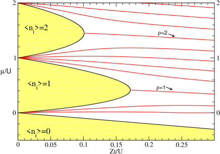
Figure 1: Mean field phase diagram in the $(\mu/U,Zt/U)$ plane for the boson Hubbard model (1).

I.2 Phase Diagram for the pure case

The phase-diagram of Eq. (1) has been obtained using several equivalent approaches. Sheshadri et al. Sheshadri et al. (1993) decouple the hopping term in the following manner:

$$\hat{\Phi}^{\dagger}_{\bf r}\hat{\Phi}_{\bf r^{\prime}}=\langle\hat{\Phi}^{\dagger}_{\bf r}\rangle\hat{\Phi}_{\bf r^{\prime}}+\langle\hat{\Phi}_{\bf r^{\prime}}\rangle\hat{\Phi}^{\dagger}_{\bf r}-\langle\hat{\Phi}^{\dagger}_{\bf r}\rangle\langle\hat{\Phi}_{\bf r^{\prime}}\rangle.$$ (5)

Using this decoupling and writing $\psi^{\star}=\langle\hat{\Phi}^{\dagger}_{\bf r}\rangle,\psi=\langle\hat{\Phi}_{\bf r}\rangle$ we see that Eq. (1) can be written as follows:

$$H_{\rm bH} \simeq \sum_{\bf r}H^{MF}_{\bf r}$$

$$H^{MF}_{\bf r} = \left(\frac{U}{2}\hat{n}_{\bf r}(\hat{n}_{\bf r}-1)-\mu\hat{n}_{\bf r}\right)$$ (6)

$$-Zt(\psi^{\star}\hat{\Phi}_{\bf r}+\psi\hat{\Phi}^{\dagger}_{\bf r}-|\psi|^{2})\ .$$

Here $Z$ is the coordination number. In the number basis $H^{MF}_{\bf r}$ is non-diagonal but straightforward to diagonalize out to fairly large occupation numbers. In this truncated basis the ground-state energy can be determined and the optimal value of $\psi$ determined where the energy is minimized. This procedure explicitly yields the ground-state wave-function at mean-field level and hence directly the density. The superfluid density can be determined from $\rho_{s}=|\psi|^{2}$. This approach is equivalent to preceding work by Fisher et al. Fisher et al. (1989) who showed that the Mott insulating lobes with occupation $n$ could be determined by considering an action of the typical Landau form $S_{\infty}(\psi)=\beta N\frac{1}{2}r|\psi|^{2}+\ldots$, with $r$ given explicitly at $T=0$ by

$$r=2\frac{U}{Zt}-2\left(\frac{n+1}{n-\mu/U}+\frac{n}{-(n-1)+\mu/U}\right)\ .$$ (7)

The transition from the Mott insulator with occupation $n>0$ to the superfluid is in this mean field approach given by $r=0$ with solution Freericks and Monien (1996):

$$\frac{\mu}{U}=n-\frac{1}{2}-\frac{x}{2}\pm\frac{1}{2}\sqrt{1-2x(2n+1)+x^{2}}\ .$$ (8)

Here, $x=Zt/U$. For the Mott insulator with $n=0$ the transition is simply given by $\mu/U=-Zt/U$. Note that in Eq. (1) the coefficient in front of $-\sum_{i}n_{i}$ is $\mu/U+1/2$. Hence the Mott insulating lobes are not centered around their corresponding chemical potential, but are off set by 1/2. The resulting phase diagram is shown in Fig. 1 and is in quite good agreement with detailed strong-coupling expansions Freericks and Monien (1996); Niemeyer et al. (1999). In Fig. 1 Eq. (8) are shown along with detailed calculations using Eq. (6) using the approach of Ref. Sheshadri et al., 1993.

It is now straightforward to consider the Mott insulating lobes present in the quantum rotor model, Eq. (2), Eq. (3). This can be done simply by studying the limit $n\to\infty$ of Eq. (8) considering that $nZt/U$ remains finite. One immediately finds that the lobes are given by:

$$\frac{\mu}{U}=\frac{1}{2}\pm\frac{1}{2}\sqrt{1-4\frac{nZt}{U}}\ .$$ (9)

For the link-current model Eq. (3) the only non-trivial interaction comes through the global divergence-less constraint and a mean-field treatment is less straight forward. However, as outlined in Ref. Wallin et al., 1994 the coupling in the link-current model Eq. (3) is related to $t/U$ of the quantum rotor model Eq. (2) and the overall shape of the phase-diagram must therefore be the same. Since the particle number now describes the deviation from the mean the resulting phase-diagram therefore becomes completely periodic in $\mu/U$ and is schematically indicated in Fig. 2.

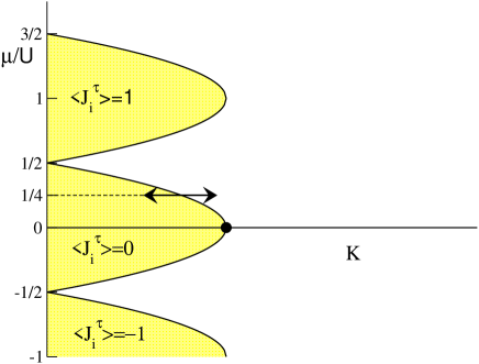
Figure 2: Schematic phase diagram in the $(\mu/U,K)$ plane for the link-current Hamiltonian (4). We have simulated the transition between the Mott insulator and the SuperFluid phase at $\mu=1/4$ (arrow in the figure).

In a previous study Alet and Sørensen (2003a), we studied the quantum phase transition at the tip of the lobe $\mu=0$ (black dot in figure (2)), where it is known that this model is in the universality class of the 3D XY model Fisher et al. (1989); Cha et al. (1991). We gave a very precise estimate of the critical point $K_{c}=0.33305(5)$ and found a value $\nu=0.670(3)$ for the correlation length critical exponent, in perfect agreement with the 3D XY universality class Campostrini et al. (2001). The dynamical critical exponent $z$ is equal to unity in this case.

In this work, we will focus on the pure case where the chemical potential is the same for all sites $\mu_{\bf r}=\mu$. In particular, we will present results obtained for a value $\mu=1/4$ of the chemical potential indicated by the arrow in Fig (2). At this point, the quantum phase transition is expected from scaling theory Fisher et al. (1989) to have a dynamical critical exponent $z=2$, and mean field values for other exponents (in particular $\nu=1/2$). As we shall see, our simulations confirm this with a good accuracy in the thermodynamic limit, but we find finite size effects that are strongly reminiscent of a first-order phase transition.

This has important implications for studies considering the relevance of disorder at this generic transition Park et al. (1999); Lee et al. (2001, 2002) since our results show that for the lattice sizes used in these studies the phase-transition appears first-order like.

II Numerical method and simulations 

II.1 Numerical method

We perform Quantum Monte Carlo simulations of the model (4) with the recently proposed geometrical worm algorithm Alet and Sørensen (2003a, b) in its ”directed” version Alet and Sørensen (2003b). We refer the interested reader to these references for more detailed explanations on this numerical technique. We also note that our algorithms are closely related to the classical worm algorithm by Prokof’ev and Svistunov Prokof’ev and Svistunov (2001) (a comparison between the two approaches has been made in Ref. Alet and Sørensen (2003b)). The most important point to underline is that these non local Monte Carlo algorithms permit the study of much larger systems with much higher precision than what was previously possible using local update schemes, thereby getting closer to the thermodynamic limit and allowing for much more precise estimates of the critical properties of the model.

II.2 Simulations

We are considering a quantum phase transition with two different correlation lengths: $\xi$ is the correlation length in spatial directions ($x,y$) and $\xi_{\tau}$, the correlation length in the $\tau$ (imaginary-time) direction. Usually one defines $\xi_{\tau}\sim\xi^{z}$, thereby defining the dynamical critical exponent $z$, not necessarily equal to unity. To respect this anisotropy between space and time directions, it is necessary to simulate the the model (4) on lattices of sizes $L$x$L$x$L_{\tau}$. Periodic boundary conditions are here assumed and the length of the lattice in the $\tau$- direction has to be chosen such that $L_{\tau}=aL^{z}$, with $a$ being the aspect ratio constant throughout the simulations. This follows from the fact that any finite-size scaling function will be a function of two arguments:

$$f(\xi/L,\xi_{\tau}/L_{\tau})=g(\xi/L,a).$$ (10)

It is therefore necessary to keep the aspect ratio $a$ constant in order to observe scaling. The value of the dynamical critical exponent is a priori unknown, and one usually has to try several values for $z$ to check the validity of theoretical predictions.

Most of the data for different values of the effective temperature $K$ were obtained with reweighting techniques Ferrenberg and Swendsen (1988) by large runs (of the order of $5\times 10^{7}$ worms) at a single value of $K$ although we in some cases combined simulations at several values of $K$ using multi-histogram techniques. We checked every time that our data were in the range of validity of the reweighting. The error bars are obtained with standard jackknife resampling techniques Efron (1982).

Among several possible thermodynamic variables, we have calculated two quantities capable of distinguishing the different phases of the system Cha et al. (1991); Sørensen et al. (1992). The first quantity is the stiffness $\rho$ which characterizes the response of the system to a twist in the boundary condition in the real space direction. In terms of the link variables, the stiffness is calculated as Cha et al. (1991); Sørensen et al. (1992); Wallin et al. (1994) :

$$\rho=\frac{1}{L_{\tau}}\langle n_{x}^{2}\rangle$$ (11)

where $n_{x}=\frac{1}{L}\sum_{{\bf r},\tau}J_{({\bf r},\tau)}^{x}$ is the winding number in the $x$ direction.

The second quantity is the compressibility $\kappa$, characterizing the fluctuation of the number of bosons in the system. This quantity is written as Sørensen et al. (1992); Wallin et al. (1994):

$$\kappa=\frac{L_{\tau}}{L^{2}}[\langle n_{\tau}^{2}\rangle-\langle n_{\tau}\rangle^{2}]$$ (12)

with $n_{\tau}=\frac{1}{L_{\tau}}\sum_{{\bf r},\tau}J_{({\bf r},\tau)}^{\tau}$ being the winding number in the time direction. This last quantity can be interpreted as the “number of bosons” in the systems. Please note that $\langle n^{\tau}\rangle$ is in general non-zero when we consider a non-zero chemical potential.

We will use finite-size scaling relation for these two quantities to localize critical points and characterize them. In two dimensions and near a critical point $K_{c}$, the scaling theory Fisher et al. (1989); Sørensen et al. (1992); Wallin et al. (1994) predicts the following finite size scaling forms for the stiffness and the compressibility :

$$\rho=L^{2-d-z}\tilde{\rho}(L^{1/\nu}\delta,a),$$ (13)

$$\kappa=L^{z-d}\tilde{\kappa}(L^{1/\nu}\delta,a),$$ (14)

where $\delta=|K-K_{c}|$ is the distance to the critical point, $\nu$ the correlation length critical exponent and where $\tilde{\rho}$ and $\tilde{\kappa}$ are scaling functions.

From these scaling forms, we see that right at the critical point $K_{c}$, in two dimensions $d=2$, the quantities $\rho L^{z}$ and $\kappa L^{2-z}$ must be independent of the system size if we choose the aspect ratio $a$ to be constant for different lattice sizes. Thus a plot of $\rho L^{z}$ or $\kappa L^{2-z}$ versus $K$ for different system sizes should show a crossing of the different curves at a single transition temperature $K_{c}$.

Moreover, by simply differentiating the equation (13) with respect to the coupling $K$, we easily see that at the critical point $K_{c}$, we have (keeping the aspect ratio constant)

$$\frac{d\rho}{dK}L^{z}\sim L^{1/\nu}$$ (15)

which is used to get the correlation length exponent. We find this way of determining $\nu$ much preferable to the traditional data collapse Kisker and Rieger (1997); Cha et al. (1991); v. Otterlo and Wagenblast (1994); v. Otterlo et al. (1995); Park et al. (1999); Lee et al. (2001, 2002), which leads to significantly more uncertainty in the determination of the critical exponents.

The derivative of $\rho$ with respect to the effective temperature $K$ can be obtained by a numerical derivation of the curve $\rho(K)$ or more preferably by calculating the thermodynamic derivative during the Monte Carlo simulations :

$$\frac{d\rho}{dK}=\langle\rho E\rangle-\langle\rho\rangle\langle E\rangle$$ (16)

where $E$ is the total energy.

III Results 

Throughout the rest of this work, we will show results obtained with the “directed” geometric worm algorithm Alet and Sørensen (2003a, b) for the link-current model (4) at an incommensurate chemical potential, $\mu=1/4$. We exclusively consider the two dimensional case with no disorder.

III.1 Determination of critical point

First, we address the question of the value of the critical point $K_{c}$ and of critical exponents. The scaling theory Fisher et al. (1989) predicts $z=2$ for the dynamical critical exponent. A plot of $\rho L^{2}$ or $\kappa$ should then show a crossing of the curves for different systems sizes at a single point. We have calculated this quantity near the previous estimate v. Otterlo and Wagenblast (1994); v. Otterlo et al. (1995) of the transition point $K_{c}\simeq 0.283(3)$ for different lattice sizes for different values of the aspect ratio : $a=1/32,1/16,1/8,1/4,1/2,1$. The small aspect ratios allows us to treat larger systems in the real space directions, gaining in precision. For all values of $a$, we simulated large systems, up to more than $3\times 10^{6}$ lattice variables. The maximum size used for different aspect ratios is indicated in table 1. A more thorough discussion of the influence of the aspect ratio follows in section III.3. Previous work v. Otterlo and Wagenblast (1994); v. Otterlo et al. (1995) using a local algorithm was limited to a maximum size $L=10$ with an aspect ratio $a=1/4$ (that is to say lattices of size $10$x$10$x$25$), whereas with the help of the geometrical worm algorithm we have been able to simulate lattices of size up to $88$x$88$x$242$ for the smallest aspect ratio used $a=1/32$ and in principle even larger lattice sizes could be studied. However, as we shall see, features present in the results obtained using these lattice sizes already tell us that the extrapolation to the thermodynamic limit will be difficult.

In Figure 3 we show results for the dependence of $\rho L^{2}$ on $K$ for different values of $L$ and the set of different aspect ratios. We see a very good crossing in all cases, and the values of $K_{c}$ (listed in table 1) only show a very slight variation with the aspect ratio, and all converge to give an estimate of $K_{c}=0.28299(2)$. As one would expect, the universal value of $\rho L^{2}$ at the critical point depends on the aspect ratio (see formula 13), and is listed in table 1.

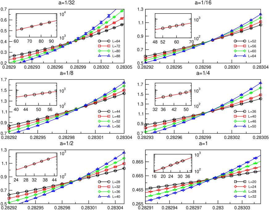
Figure 3: The scaled stiffness $\rho L^{2}$ (vertical axis) versus coupling constant $K$ (horizontal axis) for different values of aspect ratios $a$ and system sizes $L$. Lines are guides to the eye. In all cases, the curves for different systems sizes cross at the critical point, giving a precise estimate of $K_{c}$. Insets: $L^{2}\frac{d\rho}{dK}$ at $K_{c}$ as a function of system size $L$ in log-log scale. Solid lines are power-law fits.

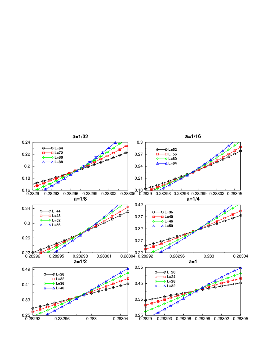
Figure 4: Compressibility $\kappa$ (vertical axis) versus coupling constant $K$ (horizontal axis) for different values of aspect ratio $a$ and system sizes $L$. Lines are guides to the eye. For all aspect ratios, a well-defined crossing of $\kappa$ for different system sizes is apparent, giving a value of $K_{c}$ agreeing with the estimate obtained from the crossing of $\rho L^{2}$ (figure 3).

In figure 4, we show our results for the compressibility $\kappa$, as a function of the effective temperature $K$, for all aspect ratios simulated. Also in this case do we observe a well defined crossing of curves for different systems sizes as one would expect from finite-size scaling theory. There is a slight variation of the estimated $K_{c}$ for the different values of the aspect ratios (see table 1), but we can safely estimate $K_{c}$ from the crossing of $\kappa$ to be $K_{c}=0.28298(2)$. This estimate of $K_{c}$ agree within error bars with the one previously obtained from the crossing of $\rho L^{2}$, even if they do not perfectly coincide. It is natural to expect such tiny deviations, and only in the thermodynamic limit should all estimates (for all different aspect ratios and for all different estimators of $K_{c}$) give the same value for $K_{c}$. The precision at which we are able to calculate $K_{c}$ largely exceeds previous studies v. Otterlo and Wagenblast (1994); v. Otterlo et al. (1995).

The fact that all our results in Fig (3) and Fig. (4) show a single well defined crossing for the large system sizes used lends strong support support to a value of $z=2$, as predicted by the scaling theory Fisher et al. (1989). This value of $z$ was implicitly used in the simulations through the choice of the lattice sizes and the well defined crossings implies that this choice was correct. In the next section (III.2) of the paper, we will show more convincing numerical evidence for this value of the dynamical critical exponent.

Another important conclusion can be drawn from the Fig (3) and Fig. (4): The fact that the estimates of $K_{c}$ from the scaling of $\rho L^{2}$ and $\kappa$ show a single well-defined $K_{c}$ allows us to rule out a very hypothetic scenario consisting of two separate transitions with an intervening exotic phase. Our results are clearly only consistent with a single well-defined transition.

We now turn to a discussion of our estimate of $\nu$ the correlation length exponent. In the inset of each of the six panels in figure 3, is shown, on a log-log scale, the size dependence of $L^{2}\frac{d\rho}{dK}$ calculated at the associated critical point $K_{c}$. From a power law fit (see equation (15)), we can estimate the correlation length critical exponent $\nu$ for all aspect ratios. The resulting estimates are also listed in table 1. In the present study we are able to simulate significantly larger systems than was previously possible in particular for small values of $a$. For $a=1/32$, we obtain a value $\nu=0.52(2)$. This estimate is in very good agreement with the mean field value $\nu=1/2$ given by the scaling theory of Fisher et al.’s theory Fisher et al. (1989). The small deviation observed for larger aspect ratios could be due to small finite size deviations as we shall discuss in the subsequent section.

To conclude this section, we would like to stress once more the importance of simulating larger systems to get more precise estimates of the critical properties. A very slow approach to the thermodynamic limit is seen for all the data in Fig. (3) and (4). For reasons of clarity we have not included the data for smaller sizes in these two figures. However, the smallest lattice sizes show a clear deviation from scaling and the lattice needed to obtain a well defined crossing of the curves is in most cases considerable. In section III.3, we will show that significant systematic finite size effects could easily give rise to an incorrect interpretation of data for certain aspect ratios.

Aspect ratio $a$	$1/32$	$1/16$	$1/8$	$1/4$	$1/2$	1
Maximum system size $L_{\rm max}$	$88$	$64$	$56$	$50$	$40$	$32$
$K_{c}$ (estimated from $\rho L^{2})$	0.282982(5)	0.282993(7)	0.283000(6)	0.282997(7)	0.282999(6)	0.282998(7)
$\rho L^{2}$ at $K_{c}$	0.397(17)	0.863(70)	1.177(60)	1.177(60)	0.867(40)	0.625(25)
$\nu$	0.52(2)	0.46(2)	0.47(2)	0.47(2)	0.47(15)	0.47(15)
$K_{c}$ (estimated from $\kappa$)	0.282975(8)	0.282980(12)	0.28300(12)	0.282991(8)	0.282996(8)	0.292987(8)
$\kappa$ at $K_{c}$	0.196(6)	0.227(9)	0.299(16)	0.328(10)	0.374(16)	0.415(15)

Table 1: Estimates of several variables for different aspect ratios used in the simulation. See text for details.

III.2 Scaling plot for $z$

In this section, we will show further numerical evidence for a value of $z=2$ for the dynamical exponent. In the context of quantum phase transitions in quantum spin glasses, Huse and coworkers Guo et al. (1994) (see also Ref. Rieger and Young (1994)) used a numerical method exploiting the anisotropy in the imaginary time direction to obtain an estimate for the dynamical exponent and the critical point. They proposed to plot the Binder cumulant versus the aspect ratio $a=L_{\tau}/L^{z}$ for different lattice sizes $L$ (i.e. they simulated systems of size $L$x$L$x$L_{\tau}$ for different $L_{\tau}$). On the basis of scaling arguments for the Binder cumulant Guo et al. (1994), it is then possible to show that all data should collapse onto a single curve at the critical point if the correct value of $z$ is used to calculate $a$ from the $L_{\tau}$ used in the simulation. Alternatively, if one for several different values of $L$ can locate a maximal value of the Binder cumulant as a function of $L_{\tau}$, then the $L_{\tau}^{max}$ associated with this maximum should scale with $L$ as $L_{\tau}^{max}\sim L^{z}$. For this to work a very precise estimate of the critical point is presumably not necessary.

We adapt this method to the quantum phase transition studied here but use the quantity $\rho L^{z}$ instead of the Binder cumulant. This quantity displays the same properties as the Binder cumulant for the application of the Huse method but suffers from the drawback that it depends on an initial assumption of $z$. Please note that, the a priori unknown value of $z$ enters implicitly in both axes in this plot. Since we have a good estimate for that $z=2$, we first calculated $\rho L^{2}$ for different $L$ and $L_{\tau}$, instead of trying less probable values for the dynamical exponent.

We show the results of our calculations in figure 5 for a value of the effective temperature equal to our previous estimate of the critical point $K_{c}=0.28299(2)$. Please note that due to computer time restrictions, we only simulated systems of moderate size ($L\leq 40$) for aspect ratios $a\leq 1/2$. Clearly all curves start to collapse into a single one, giving strong evidence that our previous estimate for $z=2$ was correct. This also confirms the validity of our previous estimate of $K_{c}$.

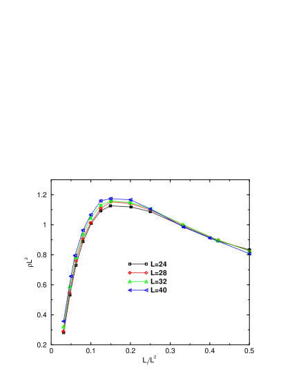
Figure 5: Scaling plot of $\rho L^{2}$ versus aspect ratio $a=\frac{L_{\tau}}{L^{2}}$ for different system sizes at $K=0.28299$.

Some deviation from a perfect collapse behavior is however present and is attributed to small finite size effects since for this calculation we only considered systems with size $L\leq 40$. In particular, small differences in the finite-size estimate of $K_{c}$ (as was shown in table 1) for different aspect ratios are most probably at the origin of this small deviation. We further discuss finite size effects in the following section.

III.3 Effects Depending on the Aspect Ratio

III.3.1 Multiple Peaks

From the results presented in the previous two sections it is clear that the approach to the thermodynamic limit is quite slow and pronounced finite-size effects are present at small lattice sizes. In the presence of long-range interactions it is known that the transition in some cases can be first-order Sørensen and Roddick (1996). In light of this result we verified whether the present transition also showed signatures of a first-order transition even though only the on-site repulsion term $U$ is included. We study this by examining in detail the energy distribution close to $K_{c}$. In all cases we take $z=2$. We examined carefully the energy distribution near the critical point for the six different values of the aspect ratio $a=1,1/2,1/4,1/8,1/16,1/32$ used in our simulations. Our results are shown in Fig. 6 where we show the probability $P(e)$ of observing an energy per site $e$ versus $e$ at the critical point $K=K_{c}$. As is evident from the results in Fig. 6 multiple peaks are present in the energy distribution for the three largest aspect ratios while the distribution of the energy for the three smaller aspect ratios show a single peak at the critical point.

Given this observation, it is instructive (see Fig. 6) to extract the contribution to $P(e)$ from the different sectors of winding number $n_{\tau}$ in the geometrical worm algorithm, which can be identified with the particle number (the number of bosons) in the system. From the results shown in Fig. 6 it is clear that for the three smallest aspect ratios, many sectors of the particle number contribute to $P(e)$ at $K=K_{c}$, in particular so for the smallest aspect ratio $a=1/32$. However for the larger aspect ratios, $a=1/4,1/2,1$, only the sectors $n_{\tau}=0,1$ and eventually $2$ contribute significantly to $P(e)$ at $K=K_{c}$. In particular, the two main peaks observed in the total histogram $P(e)$ can be clearly attributed to the contributions from the sectors with $0$ or $1$ particle in the system. Moreover, these two peaks are clearly separated.

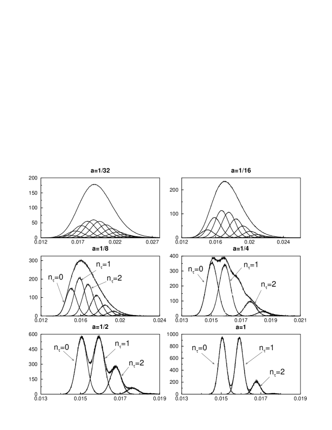
Figure 6: Probability, $P(e)$, (vertical axis) of energy per site $e$ versus $e$ (horizontal axis) observed during the Monte Carlo simulations for different aspect ratios at $K=K_{c}$. Here $L=32$ for all aspect ratios. Also shown is the contribution of each particle sector (see text) to $P(e)$. For the four larger aspect ratios, contributions of the $n_{\tau}=0$, $n_{\tau}=1$ and $n_{\tau}=2$ sectors are singled out. For reasons of clarity, we did not denote contributions of higher number of particle sectors. For the two smaller aspect ratios, the contributions of all particle sectors are also not denoted for clarity reasons.

The generic transition is clearly driven by density fluctuations as stressed by Fisher et al. Fisher et al. (1989). If this transition is second order, many particle sectors should contribute to $P(e)$ at the critical point. This is clearly the case for $a=1/32,1/16$ and to a certain extent for $a=1/8$. However, the multi-peak structure in $P(e)$ observed for $a=1/4,1/2,1$ could be interpreted as a signature of a first order phase transition. In particular, the energy gap between the contribution from the two main particle sectors (which is the energy difference between the maxima of the two main peaks) should remain non-zero in the thermodynamic limit for a first order transition. Although it would seem only a remote possibility that the order of the phase transition could change with the aspect ratio, a more thorough analysis of the signatures of a first-order transition observed for $a=1/4,1/2,1$ is clearly needed, as done in the next section.

III.3.2 Scaling of Peaks

It is not possible to draw any definitive conclusion about the order of the phase-transition from the energy distribution $P(e)$ calculated for a single $L$ for the three aspect ratios $a=1/4,1/2,1$. It is necessary to verify that this is not simply a finite size effect that will disappear as the thermodynamic limit is approached. Indeed, since we are doing simulations on a finite lattice, the density of bosons will not fluctuate continuously but only to vary it in steps of $1/L^{2}$. There have been many situations where one observes evidences for a first order transition for small lattice sizes which turns out to be second order when simulating larger systems (see for example Ref.Fukugita et al. (1990)).

We therefore made simulations for several lattices sizes for the aspect ratios $a=1/4,1/2$ and $1$. We observe for all cases a multi-peak structure in the probability distribution $P(e)$. To treat correctly the size dependence of these two peaks, one usually employs the method proposed by Lee and Kosterlitz Lee and Kosterlitz (1990) to distinguish between a first or a second order phase transition. First, with the help of reweighting techniques Ferrenberg and Swendsen (1988), we locate the temperature $K$ where the two peaks are almost of the same height not . Then we calculate at this temperature the free energy-like quantity $-\ln P(e)$.

Figure 7: The free energy-like quantity $-\ln{P(e)}$ (see text) for the three aspect ratios $a=1/4,1/2,1$ versus energy density $e$. The curves for different system sizes $L$ have been arbitrarily shifted vertically for clarity reasons. Insets : The free energy difference $\Delta F$ (see text) versus system size $L$.

Our results are shown in Fig. 7. For all the lattice sizes $L$, we still have two pronounced peaks which seem to stay of about the same size (or actually slightly increase for $a=1/4$, this is due in this specific case to the proximity of the $n_{\tau}=2$ peak, see footnote not and below) as $L$ increases. More quantitatively, we plotted in the inset of figure 7 the variation with system size of the ”free energy difference” Lee and Kosterlitz (1990) $\Delta F=\ln(\frac{P^{\rm max}(e)}{P^{\rm min}(e)})$, where $P^{\rm max}(e)$ is the height of both peaks and $P^{\rm min}(e)$ the height of the minimum between them. We see that this quantity is constant with $L$ within error bars. In Lee-Kosterlitz’s method Lee and Kosterlitz (1990), this indicates a second order phase transition.

To demonstrate this even more clearly, we also note that the separation of the peaks (the energy gap) decreases with the system size, as can be seen in Fig. 8. In particular, we observe that whereas the first peak (corresponding to $n_{\tau}=0$) stays peaked around a value $e\sim 0.015$ , the peak corresponding to $n_{\tau}=1$ is clearly shifted towards the first peak as we increase system size. Looking more carefully at the system size dependence of the energy gap $\Delta_{01}$ between the peak for the $n_{\tau}=0$ and $n_{\tau}=1$ sectors, we observe that it vanishes as $1/L^{2}$ (see insets of Fig. 8). We also observe the same scaling for the other gaps $\Delta_{02},\Delta_{03}$ corresponding to secondary peaks. This behavior clearly corresponds to a second order phase transition occurring in the thermodynamic limit. The $1/L^{2}$ scaling of the separation of the peaks is presumably simply due to the fact the particle (boson) density varies as $1/L^{2}$ between the two peaks on the finite lattice. In the thermodynamic limit the density can vary continuously. In essence, the spacing between the peaks is just a reflection of the finite energy cost associated with adding an additional boson. Moreover, we observe that the width of the peaks is decreasing with system size.

Figure 8: Scaling of the peaks in $P(e)$ for different system sizes for the aspect ratios $a=1/4,1/2,1$. Insets : Energy gap $\Delta_{01}$ separating the two first peaks as a function of $1/L^{2}$. Dashed line is a a fit to $\Delta_{01}=A/L^{2}$.

We conclude that the observed transition is a second order phase transition, but with strong finite size effects for large aspect ratios reminiscent of a first-order phase transition. These effects are presumably simply due to the fact that the density of bosons can not be varied continuously on a finite lattice and a result of the finite energy required to add an extra particle. Interestingly, these finite-size effects do not seem to be reflected too much in the estimate of the critical point $K_{c}$ obtained by crossing of $\rho L^{2}$ or the compressibility $\kappa$ and could easily have been missed in previous studies. However, it is immediately clear that if only the sector with particle number $n_{\tau}=0$ is contributing significantly at $K_{c}$ then we are effectively studying the transition occurring at a fixed particle number and not the generic, incommensurate transition. The transition at fixed particle number is equivalent to the $d+1$-$XY$ commensurate transition occuring at the tip of the MI lobes. The non-zero chemical potential is decoupled and is not taken into account correctly. The critical exponents calculated are therefore likely to be strongly influenced. This result is of significant importance for interpreting what was observed in previous simulations where only very modest lattice sizes were used v. Otterlo and Wagenblast (1994); v. Otterlo et al. (1995), and the above effects therefore likely to have been pronounced.

These finite size effects could also be of importance for previous studies of the generic transition in the presence of weak disorder Kisker and Rieger (1997); Park et al. (1999); Lee et al. (2001, 2002). The situation is perhaps less clear here since a strong enough disorder would smear the multi-peak structure observed above and enhance particle number fluctuations. However, weaker disorder would only broaden the individual peaks slightly and one would effectively be studying the influence of disorder on the commensurate transition occurring at $\mu=0$ (albeit at fixed particle number). Recent calculations Prokof’ev and Svistunov (2004, 2003) done with a variant Prokof’ev and Svistunov (2001) of the worm algorithm used in this work have shown that the situation in this case is much more subtle than previously thought, questioning the validity of older work considering the influence of weak disorder at the commensurate transition Kisker and Rieger (1997); Park et al. (1999); Lee et al. (2001, 2002). In fact, it was observed that the universal behavior only sets in at very large lattice sizes. Hence, if only weak disorder is considered for small lattice sizes one is therefore likely to observe incorrect exponents. This would explain why Park et al. Park et al. (1999) observe $\nu=0.5\pm 0.1$ at the generic transition in the presence of weak disorder violating the inequality $\nu\geq 2/d$ and would question the validity of the phase-diagram presented by Lee et al. Lee et al. (2001, 2002).

III.4 Correlation Functions

Even though in the previous two sections we have seen that the pronounced finite-size effects present at the larger lattice sizes have relatively little influence on $\kappa$ and $\rho L^{2}$ they are quite visible in the correlation functions. The correlation functions can be easily calculated using the geometrical worm algorithm as described in reference Alet and Sørensen, 2003b. From scaling theory Fisher et al. (1989); Wallin et al. (1994) we expect them to follow the following form at $K=K_{c}$:

$$C_{x}(x)\sim x^{-(d+z-2+\eta)}$$

$$C_{\tau}(\tau)\sim\tau^{-(d+z-2+\eta)/z}.$$ (17)

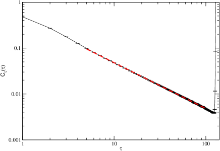
Figure 9: The $\tau$-dependent correlation function calculated on a lattice with $L=64$ and $L_{\tau}=128$ at $K_{c}$. The dashed line (hidden by the data points) indicates a fit to the form $C_{\tau}(\tau)=0.47742\tau^{-0.998}$.

In Fig. 9 we show representative results for $C_{\tau}(\tau)$ calculated at $K=K_{c}$ for the generic transition at $\mu=1/4$. There is a clear power-law dependence and it is relatively easy to extract the associated exponent $C_{\tau}(\tau)=0.47742\tau^{-0.998}$. If we take our previous estimate of $z=2$ for granted and remember that $d=2$ this would imply that $\eta=0$ consistent with mean-field behavior.

The behavior of the correlation functions in the spatial direction is much more complicated. In Fig. (10) we show representative results for $C_{x}$ calculated at $K=K_{c}$ for a system of size $L=32$ for a range of different $L_{\tau}=16,32,64,128,256,512$.

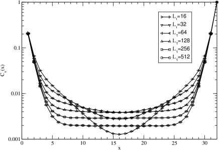
Figure 10: The x-dependent correlation function at $K=K_{c}$ for $L=32$ calculated for a range of different $L_{\tau}=16,\ldots,512$.

As is clearly evident from this figure these correlation functions do not follow a power-law behavior. Given the results presented in the previous sections this is not surprising and illustrates the difficulties associated with these finite-size effects. The deviation from power-law behavior increases dramatically with the aspect ratio. Hence, only by studying significantly larger system sizes at much smaller aspect ratios would one presumably be able to recover the expected power-law behavior. We have so far been unable to do so.

IV Conclusion 

In conclusion, we have in the present paper presented large-scale numerical results for the SF-I transition occurring in the boson Hubbard model at an incommensurate chemical potential $\mu=1/4$ obtained using the “directed” version of the recently developed geometrical worm algorithm Alet and Sørensen (2003a, b). By carefully analyzing the probability distribution $P(e)$ of the energy density at $K=K_{c}$ for different values of the aspect ratio, we showed that strong finite-size effects, reminiscent of a first order transition are present for the larger aspect ratios. These effects disappear in the thermodynamic limit and the transition is indeed second order with mean field exponents as predicted by scaling theory Fisher et al. (1989). However, if only small lattice sizes are used then these effects are pronounced and would imply that the chemical potential is not taken into account correctly, resulting in the associated critical exponents being calculated incorrectly. Finally, we note that amplitude fluctuations, absent from the Hamiltonian Eq. (4) used here, could be important at the generic transition as recent studies indicate Chamon and Nayak (2000).