Experimental realization of the one qubit Deutsch-Jozsa algorithm in a quantum dot

Abstract

We perform quantum interference experiments on a single self-assembled semiconductor quantum dot. The presence or absence of a single exciton in the dot provides a qubit that we control with femtosecond time resolution. We combine a set of quantum operations to realize the single-qubit Deutsch-Jozsa algorithm. The results show the feasibility of single qubit quantum logic in a semiconductor quantum dot using ultrafast optical control.

Time-resolved optical spectroscopy in semiconductor quantum dots has recently progressed toward the full quantum control of excitons trapped inside a single dot.Bonadeo et al. (1998); Stievater et al. (2001); Zrenner et al. (2002); Htoon et al. (2002) These advances have stimulated proposals to use excitons in quantum dots as quantum bits Troiani et al. (2000); Chen et al. (2001); Biolatti et al. (2002) for implementation of quantum computing. Very recently, the ability to operate a two-qubit gate using exciton and biexciton states was demonstrated in a single quantum dot.Li et al. (2003) These achievements represent a step toward an all-optical implementation of quantum computing using excitonic qubits. The first algorithm that comes to mind in order to check the feasibility of quantum computation in this context is the Deutsch-Jozsa (DJ) algorithm.Deutsch and Jozsa (1992) This algorithm is one of the simplest quantum algorithms that provides an exponential speed-up with respect to classical algorithms. As such, it has been extensively studied and has been used in experimental demonstrations of simple quantum computation in a variety of systems. Chuang et al. (1998); Linden et al. (1998); Gulde et al. (2003) In this Rapid Communication we report the experimental realization of the DJ algorithm for a single qubit using an optimized version of the algorithmCollins et al. (1998).

The Deutsch problem Deutsch and Jozsa (1992) involves global properties of binary functions on a subset of the natural numbers. Given a natural number $N$, we can define a set called $X_{N}$ with all the natural numbers that can be represented with $N$ bits. A binary function $f:X_{N}\to\left\{{0,1}\right\}$ is called balanced if it returns $0$ for exactly half of the elements of $X_{N}$ and $1$ for the other half. Given a function that is either balanced or constant, the Deutsch problem consists of finding out which type it is. A general classical algorithm requires evaluating the function on more than half of the elements, requiring at least $2^{N-1}+1$ evaluations. This causes the classical run time to grow exponentially with the input size. The Deutsch-Jozsa algorithm provides a way to solve the Deutsch problem on a quantum computer using a quantum subroutine that evaluates $f$. The problem and its solution provide an example of Oracle-based quantum computation.Berthiaume and Brassard (1994); Bennett et al. (1997) It is assumed that a quantum subroutine or Oracle contains the information about the unknown function. The algorithm gives a recipe on how to prepare (encoding) and read out (decoding) the qubit in an efficient way. In an experimental demonstration, we have not only to implement the algorithm (encoding and decoding operations), but we also have to build the Oracle. The specific structure of the Oracle, encoding and decoding is not unique and several versions can be found in the literature.Deutsch and Jozsa (1992); Chuang and Yamamoto (1995); Cleve et al. (1998); Collins et al. (1998). The one we are using hereCollins et al. (1998) allows us to implement the $N$=1 case with a single qubit.

Figure 1: Optimized version of the Deutsch-Jozsa algorithm.

Figure 1 shows a quantum circuit depiction of the algorithm. This circuit uses the following quantum transformations:

1. A Hadamard transformation independently applied to each qubit, $\hat{H}^{\otimes N}=\hat{H}\otimes\ldots\otimes\hat{H}$. A single qubit transformation is represented by

   $$\hat{H}=\frac{1}{\sqrt{2}}\left[\begin{array}[]{rr}1&1\\ 1&-1\\ \end{array}\right].$$ (1)

2. A $f$-controlled gate, whose operation is defined as

   $$\hat{U}_{f}|{x}\rangle=(-1)^{f(x)}|{x}\rangle.$$ (2)

The final step in the algorithm measures the expectation value of the $|{0}\rangle\langle{0}|$ operator. This expectation value for a constant function will be equal to $1$ while for a balanced function it will be equal to $0$. When $N$=1 there are only four possible functions $f_{j}:\left\{{0,1}\right\}\to\left\{{0,1}\right\}$:

$$f_{1}(x)=0,$$ (3)

$$f_{2}(x)=1,$$ (4)

$$f_{3}(x)=x,$$ (5)

$$\mbox{and}~{}f_{4}(x)=1-x.$$ (6)

Of these four, $f_{1}$ and $f_{2}$ are constant while $f_{3}$ and $f_{4}$ are balanced. The explicit matrix forms of the $\hat{U}_{f}$ operators are:

$$\hat{U}_{f_{1}}=\left[\begin{array}[]{rr}1&0\\ 0&1\\ \end{array}\right]=\hat{I},\quad\hat{U}_{f_{2}}=-\left[\begin{array}[]{rr}1&0\\ 0&1\\ \end{array}\right]=-\hat{I},$$ (7)

$$\hat{U}_{f_{3}}=\left[\begin{array}[]{rr}1&0\\ 0&-1\\ \end{array}\right]=\hat{\sigma_{z}},~{}\mbox{and}~{}\hat{U}_{f_{4}}=-\left[\begin{array}[]{rr}1&0\\ 0&-1\\ \end{array}\right]=-\hat{\sigma_{z}}.$$ (8)

We can see that the balanced functions share the same $f$-controlled operator except for a global phase. This is also true for the constant functions. If the qubit is initially in the state $|{0}\rangle$, the encoding transformation consists in one Hadamard operation that transforms the qubit to

$$\frac{1}{\sqrt{2}}(|{0}\rangle+|{1}\rangle).$$ (9)

By applying $\hat{U}_{f_{j}}$ to the state in Eq. 9 we obtain

$$\hat{U}_{f_{j}}\frac{1}{\sqrt{2}}(|{0}\rangle+|{1}\rangle)=\frac{1}{\sqrt{2}}[(-1)^{f_{j}(0)}|{0}\rangle+(-1)^{f_{j}(1)}|{1}\rangle].$$ (10)

For a constant function this gives

$$(-1)^{f_{j}(0)}\frac{1}{\sqrt{2}}(|{0}\rangle+|{1}\rangle),$$ (11)

while for a balanced function we get

$$(-1)^{f_{j}(0)}\frac{1}{\sqrt{2}}(|{0}\rangle-|{1}\rangle).$$ (12)

As a decoding procedure, we apply again the Hadamard transformation. We obtain

$$(-1)^{f_{j}(0)}|{0}\rangle$$ (13)

for a constant function, and

$$(-1)^{f_{j}(0)}|{1}\rangle$$ (14)

for a balanced function. Therefore, by measuring one of the two states, one can decide in a deterministic way to which class $f$ belongs. We remark that if we were to obtain an answer using only classical operations, we would need to evaluate the unknown $f$ function twice, obtaining both $f(0)$ and $f(1)$ and comparing them. Conversely, the described quantum procedure only requires one call of the quantum subroutine $\hat{U}_{f}$ is needed. Therefore the $N$=1 case of the DJ already shows that the quantum algorithm outperforms its classical counterpart by a factor of two in the number of evaluations.

We have been able to implement the single-qubit Deutsch-Jozsa algorithm discussed above using the excitonic states of a self-assembled InGaAs quantum dot as a qubit. The level scheme we used is depicted in Fig. 2. The absence of an exciton is taken as the $|{0}\rangle$ state of the qubit, while the first excited excitonic state is taken as $|{1}\rangle$. The $|{1}\rangle$ state population is monitored via a non-radiative transition to the exciton ground state (labeled as $|{1^{\prime}}\rangle$) whose radiative recombination is recorded using a micro-photoluminescence setup.Htoon et al. (1999, 2000, 2001, 2002); Muller et al. (2004)

Figure 2: Quantum level structure. The excitonic ground state and first excited state are labeled $|{1^{\prime}}\rangle$ and $|{1}\rangle$ respectively. The state $|{0}\rangle$ corresponds to the absence of an exciton in the quantum dot.

We will use two different unitary transformations to realize the Deutsch-Jozsa algorithm: a $\frac{\pi}{2}$ single qubit rotation and a phase shift. The corresponding explicit matrix forms are:

$$\hat{U}_{\frac{\pi}{2}}=\frac{1}{\sqrt{2}}\left[\begin{array}[]{rr}1&-1\\ 1&1\\ \end{array}\right]$$ (15)

and

$$\hat{U}(\phi)=\left[\begin{array}[]{rr}e^{-i\frac{\phi}{2}}&0\\ 0&e^{i\frac{\phi}{2}}\\ \end{array}\right].$$ (16)

The single qubit rotation is realized by a $\pi/2$ pulse resonant with the $|{0}\rangle$ to $|{1}\rangle$ transition. We use the rotating wave approximation and the qubit is defined in the rotating frame. The phase gate $\hat{U}(\phi)$ is realized by controlling the phase of the optical pulses with respect to the first pulse which is used as a reference. This is achieved experimentally by a piezoelectric translation stage that controls the phase locking between the pulses. By choosing specific values for $\phi$, $\hat{U}(\phi)$ becomes equivalent to the $f$-controlled operators, as shown in Table I. In this version of the algorithm, the Oracle distinguishes the operations within the same class only by a global phase in the single qubit space. We can always think about an additional reference qubit in the Oracle to make this phase physically measurable. However, this reference qubit will never come into play in the real algorithm since it is part of the internal structure of the Oracle.

Notice that although $\hat{U}_{\frac{\pi}{2}}$ and $\hat{H}$ behave in a similar way, they are not the same operator. It is easy to show that the only effect of this change is that the interpretation of the final result has to exchange balanced with constant functions. We can think about the quantum evolution of the qubit during the algorithm using the picture of a pseudo-spin in the Bloch sphere. The first pulse corresponds to an effective magnetic field in the $+{\bf y}$ direction that brings the pseudo-spin from $-{\bf z}$ to the $-{\bf x}$ direction. The phase shift corresponds to a rotation of the pseudo-spin around the ${\bf z}$ axis of multiples of $\pi$. The second pulse will bring the pseudo-spin back to $-{\bf z}$ in the case of a balanced function (by destructive interference), and to $+{\bf z}$ in the case of a constant function. In this picture the $N$=1 Deutsch algorithm shows clearly its equivalence to a Mach-Zehnder interferometer experiment.Cleve et al. (1998)

The sample consisted of In_0.5Ga_0.5As MBE grown self-assembled quantum dots, kept at a temperature of 5 K inside a continuous flow liquid helium cryostat. The quantum dots were resonantly excited with pulses from a mode-locked Ti:Sa laser. The pulses were linearly polarized in a way to make sure only one state out of an anisotropy induced doublet was excited.Muller et al. (2004) By using a spectrometer combined with a two-dimensional liquid nitrogen cooled charge-coupled device (CCD) array detector, we were able to detect the integrated photoluminescence signals of many quantum dots at the same time.Htoon et al. (2000) This enabled us to search for a quantum dot with a large enough dipole moment (and thus a good signal-to-noise ratio) and a dephasing time larger than 20 ps for the excited state, which is the case for about 1% of the dots. We did not select any specific polarization at the detection.

The use of the excitonic ground state photoluminescence as the means of detection prevented us from being able to use this state as the $|{1}\rangle$ state of our qubit. This entailed a severe decrease in the dephasing time of the qubit, as the non-radiative decay from the excited state to the exciton ground state (necessary for our detection scheme to work) puts an upper bound in the coherence time of the exciton. This upper bound is significant, since measured dephasing times for excitonic ground states are in the order of hundreds of picosecondsBorri et al. (2001); Birkedal et al. (2001); Bayer and Forchel (2002) while those for carefully chosen excited states (i.e. no further than approximately 20 meV apart from the corresponding ground state) range in the tens of picoseconds.Htoon et al. (2001)

The actual implementation of the algorithm was similar to that of standard wave packet interferometry measurements,Bonadeo et al. (1998); Kamada et al. (2001) but in the nonlinear excitation regime.Htoon et al. (2002) In order to establish the appropriate excitation intensity for a $\frac{\pi}{2}$ pulse, we first recorded Rabi Oscillations of the excited state.Kamada et al. (2001); Htoon et al. (2002) We also performed a low intensity wave packet interferometry measurement to estimate the dephasing time of the quantum dot.Bonadeo et al. (1998); Kamada et al. (2001) In that experiment, the photoluminescence signal is proportional to the wavefunction autocorrelation. By fitting the decay of the autocorrelation signal with an exponential function we were able to measure the dephasing time of the exciton in the dot, obtaining 40 ps as a result.

In the main experiment, the time delay between two identical resonant $\frac{\pi}{2}$ laser pulses (approximately 5 ps long) was scanned while simultaneously recording the photoluminescence. A mechanical translation stage controlled the coarse delay between the two pulses while a piezoelectric stage changed the fine delay. The fine delay is used to control the phase shift of the second pulse with respect to the first one. It can be mapped to the relative phase by the relation $\phi=\omega_{0}\tau$, where $\hbar\omega_{0}$ is the laser energy, and has been calibrated by performing wavepacket interferometry at low intensity on the quantum dot, keeping the mechanical stage at a fixed position.

The encoding and decoding consist of the preparation of the two pulses with the same phase. We can imagine that the Oracle controls the fine delay knob, and, by changing the relative phase, determines which one of the four functions is being implemented. Figure 3a shows the intensity of the detected photoluminescence as a function of the coarse delay between the two pulses. The lower and upper signals correspond to constructive and destructive interference depending on the relative phase of the two pulses. The contrast between the maxima and minima of the signal decreases as the delay between the pulses approaches the dephasing time of the dot (40 ps), leading to lower fidelities. Figures 3b-e describe the detailed behavior of the signal for various values of the phase difference between the two pulses.

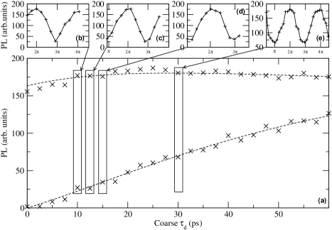
Figure 3: Central plot: Envelope of the photoluminescence (PL) as a function of the coarse pulse delay. PL signals as a function of the phase difference between the two pulses are shown in the insets.

We can now interpret this result in terms of the DJ quantum algorithm. As expected, the maximum population at $|{1}\rangle$ (that is maximum photoluminescence) occurs for even numbers of $\pi$ in the relative phase between the two pulses, corresponding to the constant quantum subroutines $\hat{U}_{f_{1,2}}$. On the other hand, minima occur for odd numbers of $\pi$ in the phase shift between the two pulses, corresponding to the balanced quantum subroutines $\hat{U}_{f_{3,4}}$. The probability of successfully solving the problem is related to the contrast of the maxima and minima in the interference process. We remark that the first three insets in Fig. 3 (all with a delay between the pulses between 10 and 20 ps) have a contrast of the order of 75%. This implies a fidelity for the quantum operations comparable to other similar implementations.Li et al. (2003) The fidelity is mainly limited by the dephasing time of the excited excitonic state of the quantum dot. Making the coarse delay between the pulses as short as possible gives the best fidelity (as can be seen in Fig. 3), but this delay must be no shorter than twice the excitation pulse width, so that any optical interference arising out of the overlap of the two pulses is negligible. Also, a detection scheme able to resonantly excite and then measure the exciton ground state would allow for much larger fidelities, due to the increased coherence times.

Experimental phase shift	Operation
$4n\pi$	$\hat{U}_{f_{1}}$
$\pi+4n\pi$	$-i\hat{U}_{f_{3}}$
$2\pi+4n\pi$	$\hat{U}_{f_{2}}$
$3\pi+4n\pi$	$-i\hat{U}_{f_{4}}$

Table 1: Experimental phase shift and their implemented operations

By using an interferometric set-up on an excitonic qubit system, we have been able to implement the single-qubit Deutsch-Jozsa algorithm. Although the 1-qubit version of the algorithm does not show all the features of Quantum Computing (in particular entanglement), it is an experimental demonstration of simple quantum computation, including superpositions and interference, in a solid state system.