Exponential distribution of financial returns at mesoscopic time lags: a new stylized fact

Abstract

We study the probability distribution of stock returns at mesoscopic time lags (return horizons) ranging from about an hour to about a month. While at shorter microscopic time lags the distribution has power-law tails, for mesoscopic times the bulk of the distribution (more than 99% of the probability) follows an exponential law. The slope of the exponential function is determined by the variance of returns, which increases proportionally to the time lag. At longer times, the exponential law continuously evolves into Gaussian distribution. The exponential-to-Gaussian crossover is well described by the analytical solution of the Heston model with stochastic volatility.

1 Introduction

The empirical probability distribution functions (EDFs) for different assets have been extensively studied by the econophysics community in recent years [1, 2, 3, 4, 5, 6, 7, 8, 9, 10]. Stock and stock-index returns have received special attention. We focus here on the EDFs of the returns of individual large American companies from 1993 to 1999, a period without major market disturbances. By ‘return’ we always mean ‘log-return’, the difference of the logarithms of prices at two times separated by a time lag $t$.

The time lag $t$ is an important parameter: the EDFs evolve with this parameter. At micro lags (typically shorter than one hour), effects such as the discreteness of prices and transaction times, correlations between successive transactions, and fluctuations in trading rates become important. Power-law tails of EDFs in this regime have been much discussed in the literature before [2, 3]. At ‘meso’ time lags (typically from an hour to a month), continuum approximations can be made, and some sort of diffusion process is plausible, eventually leading to a normal Gaussian distribution. On the other hand, at ‘macro’ time lags, the changes in the mean market drifts and macroeconomic ‘convection’ effects can become important, so simple results are less likely to be obtained. The boundaries between these domains to an extent depend on the stock, the market where it is traded, and the epoch. The micro-meso boundary can be defined as the time lag above which power-law tails constitute a very small part of the EDF. The meso-macro boundary is more tentative, since statistical data at long time lags become sparse.

The first result is that we extend to meso time lags a stylized fact known since the 19th century [11] (quoted in [12]): with a careful definition of time lag $t$, the variance of returns is proportional to $t$.

The second result is that log-linear plots of the EDFs show prominent straight-line (tent-shape) character, i.e. the bulk (about 99%) of the probability distribution of log-return follows an exponential law. The exponential law applies to the central part of EDFs, i.e. not too big log-returns. For the far tails of EDFs, usually associated with power laws at micro time lags, we do not have enough statistically reliable data points at meso lags to make a definite conclusion. Exponential distributions have been reported for some world markets [4, 5, 6, 7, 8, 9, 10] and briefly mentioned in the book [1] (see Fig. 2.12). However, the exponential law has not yet achieved the status of a stylized fact. Perhaps this is because influential work [2, 3] has been interpreted as finding that the individual returns of all the major US stocks for micro to macro time lags have the same power law EDFs, if they are rescaled by the volatility.

The Heston model is a plausible diffusion model with stochastic volatility, which reproduces the timelag-variance proportionality and the crossover from exponential distribution to Gaussian. This model was first introduced by Heston, who studied option prices [13]. Later Drăgulescu and Yakovenko (DY) derived a convenient closed-form expression for the probability distribution of returns in this model and applied it to stock indexes from 1 day to 1 year [4]. The third result is that the DY formula with three lag-independent parameters reasonably fits the time evolution of EDFs at meso lags.

2 Probability distribution of log-returns in the Heston model

In this section, the Heston model [13] and the DY formula [4] are briefly summarized. The price $S_{t}$ of a model stock obeys the stochastic differential equation of multiplicative Brownian motion: $dS_{t}=\mu S_{t}\,dt+\sqrt{v_{t}}S_{t}\,dW_{t}^{(1)}$. Here the subscript $t$ indicates time dependence, $\mu$ is the drift parameter, $W_{t}^{(1)}$ is a standard random Wiener process, and $v_{t}$ is the fluctuating time-dependent variance. The detrended log-return is defined as $x_{t}=\ln(S_{t}/S_{0})-\mu t$, although detrending is a minor correction at meso lags. In the Heston model, the variance $v_{t}$ obeys the mean-reverting stochastic differential equation:

$$dv_{t}=-\gamma(v_{t}-\theta)\,dt+\kappa\sqrt{v_{t}}\,dW_{t}^{(2)}.$$ (1)

Here $\theta$ is the long-time mean of $v$, $\gamma$ is the rate of relaxation to this mean, and $\kappa$ is the variance noise. We take the Wiener processes $W_{t}^{(1,2)}$ to be uncorrelated.

The DY formula [4] for the probability density function (PDF) $P_{t}(x)$ is:

$$P_{t}(x)=\int\limits_{-\infty}^{+\infty}\frac{dk}{2\pi}\,e^{ikx+F_{\tilde{t}}(k)},\;F_{\tilde{t}}(k)=\frac{\alpha\tilde{t}}{2}-\alpha\ln\left[\cosh\frac{\Omega\tilde{t}}{2}+\frac{\Omega^{2}+1}{2\Omega}\sinh\frac{\Omega\tilde{t}}{2}\right],$$ (2)

$$\tilde{t}=\gamma t,\quad\alpha=2\gamma\theta/\kappa^{2},\quad\Omega=\sqrt{1+(k\kappa/\gamma)^{2}},\quad\sigma_{t}^{2}\equiv\langle x_{t}^{2}\rangle=\theta t.$$ (3)

The variance $\sigma_{t}^{2}\equiv\langle x_{t}^{2}\rangle$ (3) of the PDF (2) increases linearly in time, while $\langle x_{t}\rangle=0$. The three parameters of the model are $\gamma$, $\theta$ and $\alpha$. At short and long time lags, the PDF (2) reduces to exponential (if $\alpha=1$) and Gaussian [4]:

$$P_{t}(x)\propto\left\{\begin{array}[]{ll}\exp(-|x|\sqrt{2/\theta t}),&\quad\tilde{t}=\gamma t\ll 1,\\ \exp(-x^{2}/2\theta t),&\quad\tilde{t}=\gamma t\gg 1.\end{array}\right.$$ (4)

In both limits, it scales with the volatility: $P_{t}(x)=f(x/\sqrt{\langle x_{t}^{2}\rangle})=f(x/\sqrt{\theta t})$, where $f$ is the exponential or the Gaussian function.

3 Data analysis and discussion

We analyzed the data from Jan/1993 to Jan/2000 for $27$ Dow companies, but show results only for four large cap companies: Intel (INTC) and Microsoft (MSFT) traded at NASDAQ, and IBM and Merck (MRK) traded at NYSE. We use two databases, TAQ to construct the intraday returns and Yahoo database for the interday returns. The intraday time lags were chosen at multiples of 5 minutes, which divide exactly the 6.5 hours (390 minutes) of the trading day. The interday returns are as described in [4, 5] for time lags from 1 day to 1 month = 20 trading days.

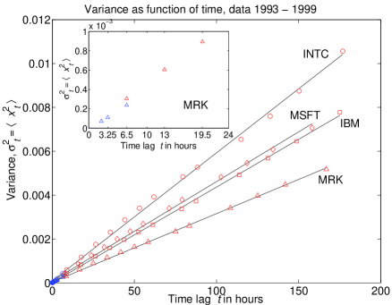
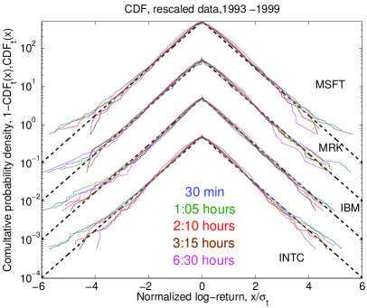
Figure 1: Left panel: Variance $\langle x_{t}^{2}\rangle$ vs. time lag $t$. Solid lines: Linear fits $\langle x_{t}^{2}\rangle=\theta t$. Inset: Variances for MRK before adjustment for the effective overnight time $T_{n}$. Right panel: Log-linear plots of CDFs vs. $x/\sqrt{\theta t}$. Straight dashed lines $-|x|\sqrt{2/\theta t}$ are predicted by the DY formula (4) in the short-time limit. The curves are offset by a factor of 10.

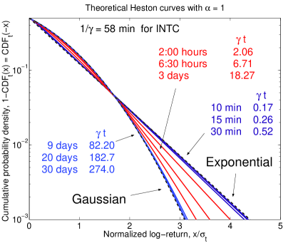
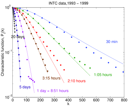
Figure 2: Left panel: Theoretical CDFs for the Heston model plotted vs. $x/\sqrt{\theta t}$. The curves interpolate between the short-time exponential and long-time Gaussian scalings. Right panel: Comparison between empirical (points) and the DY theoretical (curves) characteristic functions $\tilde{P}_{t}(k)$.

In order to connect the interday and intraday data, we have to introduce an effective overnight time lag $T_{n}$. Without this correction, the open-to-close and close-to-close variances would have a discontinuous jump at 1 day, as shown in the inset of the left panel of Fig. 1. By taking the open-to-close time to be 6.5 hours, and the close-to-close time to be 6.5 hours + $T_{n}$, we find that variance $\langle x_{t}^{2}\rangle$ is proportional to time $t$, as shown in the left panel of Fig. 1. The slope gives us the Heston parameter $\theta$ in Eq. (3). $T_{n}$ is about 2 hours (see Table 1).

In the right panel of Fig. 1, we show the log-linear plots of the cumulative distribution functions (CDFs) vs. normalized return $x/\sqrt{\theta t}$. The $\makebox{CDF}_{t}(x)$ is defined as $\int_{-\infty}^{x}P_{t}(x^{\prime})\,dx^{\prime}$, and we show $\makebox{CDF}_{t}(x)$ for $x<0$ and $1-\makebox{CDF}_{t}(x)$ for $x>0$. We observe that CDFs for different time lags $t$ collapse on a single straight line without any further fitting (the parameter $\theta$ is taken from the fit in the left panel). More than 99% of the probability in the central part of the tent-shape distribution function is well described by the exponential function. Moreover, the collapsed CDF curves agree with the DY formula (4) $P_{t}(x)\propto\exp(-|x|\sqrt{2/\theta t})$ in the short-time limit for $\alpha=1$ [4], which is shown by the dashed lines.

Table 1: Fitting parameters of the Heston model with $\alpha=1$ for the 1993–1999 data.

	$\gamma$	$1/\gamma$	$\theta$	$\mu$	$T_{n}$
	${1\over{\rm hour}}$	hour	${1\over{\rm year}}$	${1\over{\rm year}}$	hour
INTC	$1.029$	$0\colon 58$	$13.04\%$	$39.8\%$	$2\colon 21$
IBM	$0.096$	$10\colon 25$	$9.63\%$	$35.3\%$	$2\colon 16$
MRK	$0.554$	$1\colon 48$	$6.57\%$	$29.4\%$	$1\colon 51$
MSFT	$1.284$	$0\colon 47$	$9.06\%$	$48.3\%$	$1\colon 25$

Because the parameter $\gamma$ drops out of the asymptotic Eq. (4), it can be determined only from the crossover regime between short and long times, which is illustrated in the left panel of Fig. 2. We determine $\gamma$ by fitting the characteristic function $\tilde{P}_{t}(k)$, a Fourier transform of $P_{t}(x)$ with respect to $x$. The theoretical characteristic function of the Heston model is $\tilde{P}_{t}(k)=e^{F_{\tilde{t}}(k)}$ (2). The empirical characteristic functions (ECFs) can be constructed from the data series by taking the sum $\tilde{P}_{t}(k)={\rm Re}\sum_{x_{t}}\exp(-ikx_{t})$ over all returns $x_{t}$ for a given $t$ [14]. Fits of ECFs to the DY formula (2) are shown in the right panel of Fig. 2. The parameters determined from the fits are given in Table 1.

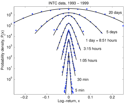
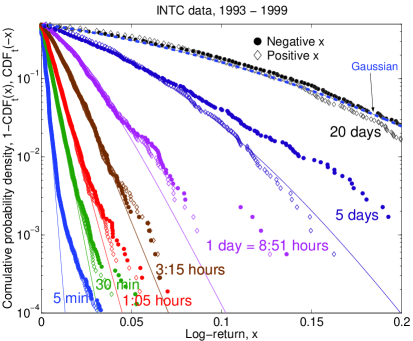
Figure 3: Comparison between the 1993–1999 Intel data (points) and the DY formula (2) (curves) for PDF (left panel) and CDF (right panel).

In the left panel of Fig. 3 we compare the empirical PDF $P_{t}(x)$ with the DY formula (2). The agreement is quite good, except for the very short time lag of 5 minutes, where the tails are visibly fatter than exponential. In order to make a more detailed comparison, we show the empirical CDFs (points) with the theoretical DY formula (lines) in the right panel of Fig. 3. We see that, for micro time lags of the order of 5 minutes, the power-law tails are significant. However, for meso time lags, the CDFs fall onto straight lines in the log-linear plot, indicating exponential law. For even longer time lags, they evolve into the Gaussian distribution in agreement with the DY formula (2) for the Heston model. To illustrate the point further, we compare empirical and theoretical data for several other companies in Fig. 4.

In the empirical CDF plots, we actually show the ranking plots of log-returns $x_{t}$ for a given $t$. So, each point in the plot represents a single instance of price change. Thus, the last one or two dozens of the points at the far tail of each plot constitute a statistically small group and show large amount of noise. Statistically reliable conclusions can be made only about the central part of the distribution, where the points are dense, but not about the far tails.

4 Conclusions

We have shown that in the mesoscopic range of time lags, the probability distribution of financial returns interpolates between exponential and Gaussian law. The time range where the distribution is exponential depends on a particular company, but it is typically between an hour and few days. Similar exponential distributions have been reported for the Indian [6], Japanese [7], German [8], and Brazilian markets [9, 10], as well as for the US market [4, 5] (see also Fig. 2.12 in [1]). The DY formula [4] for the Heston model [13] captures the main features of the probability distribution of returns from an hour to a month with a single set of parameters. We believe that econophysicists should be aware of the presence of the exponential distribution and recognize it as another “stylized fact” in the set of analytical tools for financial data analysis.

We thank Chuck Lahaie from the Robert H. Smith School of Business at UMD for help with the TAQ database.

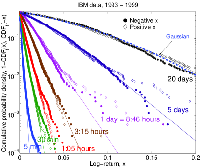
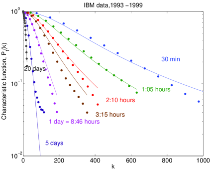
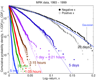
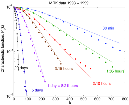
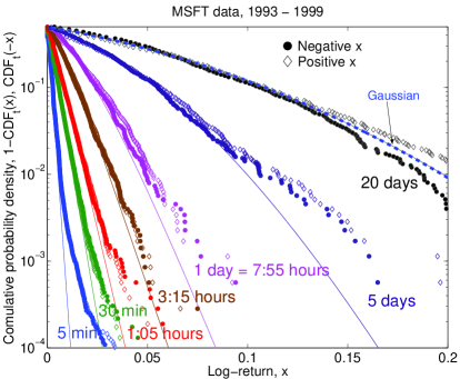
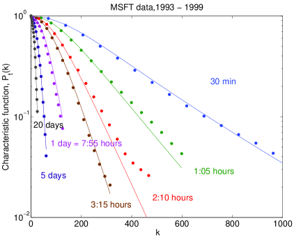
Figure 4: Comparison between empirical data (symbols) and the DY formula (2) (lines) for CDF (left panels) and characteristic function (right panels).

References

- [1] J.-P. Bouchaud and M. Potters, Theory of Financial Risks (Cambridge University Press, Cambridge, 2000).
- [2] V. Plerou, P. Gopikrishnan, L. N. Amaral, M. Meyer, and H. E. Stanley, Phys. Rev. E 60, 6519 (1999).
- [3] P. Gopikrishnan, V. Plerou, L. A. N. Amaral, M. Meyer, and H. E. Stanley, Phys. Rev. E 60, 5305 (1999).
- [4] A. Drăgulescu and V. M. Yakovenko, Quantitative Finance 2, 443 (2002).
- [5] A. C. Silva and V. M. Yakovenko, Physica A 324, 303 (2003).
- [6] K. Matia, M. Pal, H. Salunkay, and H. E. Stanley, Europhys. Letters 66 (2004) 909.
- [7] T. Kaizoji and M. Kaizoji, Advances in Complex Systems 6, 303 (2003).
- [8] R. Remer and R. Mahnke, Application of Heston model and its solution to German DAX data (talk presented at the APFA-4 conference, 2003).
- [9] R. Vicente, C. M. de Toledo, V. B. P. Leite, and N. Caticha, preprint http://lanl.arXiv.org/abs/cond-mat/0402185.
- [10] L. C. Miranda and R. Riera, Physica A 297, 509 (2001).
- [11] J. Regnault, Calcul des Chances et Philosophie de la Bourse (Mallet-Bachelier et Castel, Paris, 1863).
- [12] M. Taqqu, Paper #134, http://math.bu.edu/people/murad/articles.html.
- [13] S. L. Heston, Review of Financial Studies 6, 327 (1993).
- [14] N. G. Ushakov, Selected Topics in Characteristic Functions (VSP, Utrecht, 1999).