Bridging the ARCH model for finance and nonextensive entropy

Abstract

Engle’s ARCH algorithm is a generator of stochastic time series for financial returns (and similar quantities) characterized by a time-dependent variance. It involves a memory parameter $b$ ($b=0$ corresponds to no memory), and the noise is currently chosen to be Gaussian. We assume here a generalized noise, namely $q_{n}$-Gaussian, characterized by an index $q_{n}\in{\cal R}$ ($q_{n}=1$ recovers the Gaussian case, and $q_{n}>1$ corresponds to tailed distributions). We then match the second and fourth momenta of the ARCH return distribution with those associated with the $q$-Gaussian distribution obtained through optimization of the entropy $S_{q}=\frac{1-\sum_{i}{p_{i}}^{q}}{q-1}$, basis of nonextensive statistical mechanics. The outcome is an analytic distribution for the returns, where an unique $q\geq q_{n}$ corresponds to each pair $(b,q_{n})$ ($q=q_{n}$ if $b=0$). This distribution is compared with numerical results and appears to be remarkably precise. This system constitutes a simple, low-dimensional, dynamical mechanism which accommodates well within the current nonextensive framework.

Time series are ubiquitous in nature. They appear in geoseismic phenomena, El Niño, finance, electrocardio- and electroencephalographic profiles, among many others. Some of these series can be constructed by using, for successive values ot time $t$, random variables associated with the same distribution for all times: they are called homoskedastic. Such is the case of the ordinary Brownian motion. But many phenomena exist in nature which do not accomodate with such a property, i.e., the distribution associated with each value of $t$ depends on $t$. Such random variables are then called heteroskedastic. A simple illustration would be to use say a centered Gaussian at all steps, but with a randomly varying width.

Nowadays, time series that are intensively studied are the financial ones, where nonstationary volatility (technical name for second-order moment of say returns) is a common feature [1, 2, 3]. In order to mimic explicitly and analyze this type of time series, R.F. Engle introduced in 1982 the autoregressive conditional heteroskedasticity (ARCH) process[4]. Its prominence can be measured by its wide use, by the amount of its extensions introduced later [5, 6], and — last but not least — by the fact that the 2003 Nobel Prize for Economics was awarded to Engle “for methods of analyzing economic time series with time-varying volatility (ARCH)”. This and similar processes are commonly used in the implementation of asset pricing theories, market microstructure models, and pricing derivative assets [6, 7] (see also [8]). Specifically, the ARCH($s$)[4] process generates, for the returns $z_{t}$, a discrete time series whose variance $\sigma_{t}^{2}$, at each time step, depends linearly on the $s$ previous values of $[z_{t}]^{2}$. It is defined as follows:

$$\left\{\begin{array}[]{c}z_{t}=\sigma_{t}\;\omega_{t},\\ \sigma_{t}^{2}=a+\sum_{i=1}^{s}b_{i}\;z_{t-i}^{2}\;,\end{array}\right.$$ (1)

or, equivalently,

$$\left\{\begin{array}[]{c}z_{t}=\sqrt{a+\sum_{i=1}^{s}b_{i}\;z_{t-i}^{2}}\,\;\omega_{t}\\ \sigma_{t}^{2}=a+\sum_{i=1}^{s}b_{i}\;\sigma^{2}_{t-i}\;\omega^{2}_{t-i}\;,\end{array}\right.$$ (2)

where $a,b_{i},\sigma_{t}\geq 0$, and $\omega_{t}$ represents an independent and identically distributed stochastic process with mean value null and unit variance, (i.e., $\left\langle\omega_{t}\right\rangle=0$ and $\left\langle\omega_{t}^{2}\right\rangle=1$), currently chosen to follow a Gaussian distribution, but other choices are possible. In this manuscript we will discuss in detail the usual case $s=1$, ARCH(1), which will be from now on simply designated by ARCH. In general, the distribution, $P_{n}\left(\omega\right)$, together with parameters $a$ and $\{b_{i}\}$, specify the particular ARCH process ($n$ stands for noise).

As can be seen from Eqs. (2), parameters $\{b_{i}\}$ characterize the memory mechanism. For $b_{i}=0\;(\forall i)$, there is no memory effect, and consequently the ARCH process for returns reduces to generating the noise $\omega_{t}$ (multiplied by $\sqrt{a}$). We can verify that, in general, $\langle z_{t}\rangle=\langle\sigma_{t}\rangle\langle\omega_{t}\rangle=0$, and $\langle z_{t}\,z_{t^{\prime}}\rangle=\langle\sigma_{t}\,\sigma_{t^{\prime}}\rangle\langle\omega_{t}\,\omega_{t^{\prime}}\rangle=\langle\sigma_{t}\,\sigma_{t^{\prime}}\rangle\,\delta_{tt^{\prime}}$. Therefore, even for nonvanishing $b_{i}$’s, the returns $z_{t}$ remain uncorrelated, whereas correlations do exist in the variance $\sigma_{t}^{2}$ [5]. We observe that this stochastic process captures the tendency for the so called volatility clustering, i.e., large (small) values of $z_{t}$ are followed by other large (small) values of $z_{t+1}$, but of arbitrary sign. In other words, $\langle|z_{t}|\,|z_{t^{\prime}}|\rangle$ by no means is proportional to $\delta_{tt^{\prime}}$.

Hereon we focus on ARCH(1), i.e., $b_{1}\equiv b$ and $b_{i}=0\;(i=2,\,3,...)$. From Eqs. (1) it is simple to obtain the n-th moment for the $P(z)$ stationary distributions, particularly the second moment

$$\sigma^{2}\equiv\left\langle z_{t}^{2}\right\rangle=\langle\sigma_{t}^{2}\rangle=\frac{a}{1-b}\;\;\;(b<1),$$ (3)

and the fourth moment,

$$\left\langle z^{4}\right\rangle=a^{2}\left\langle\omega_{t}^{4}\right\rangle\frac{1+b}{\left(1-b\right)\left(1-b^{2}\left\langle\omega_{t}^{4}\right\rangle\right)}\,.$$ (4)

Without loss of generality, we can assume that the ARCH procedure generates a time series with unit variance, i.e., $\sigma^{2}=1$, hence $a=1-b$. Now, for $z_{t}$, the fourth moment is numerically equal to the kurtosis $k_{x}\equiv\frac{\left\langle x^{4}\right\rangle}{\left\langle x^{2}\right\rangle^{2}}$ (a possible measure of non-gaussianity or peakedness for probability distributions), and we can easily get,

$$\left\langle z_{t}^{4}\right\rangle=k_{z}=k_{\omega}\Bigl{[}1+b^{2}\frac{k_{\omega}-1}{1-k_{\omega}b^{2}}\Bigr{]}\;\;\;\;(k_{\omega}b^{2}<1)\;,$$ (5)

It is straightforwardly verified that, whatever the form of $P_{n}\left(\omega\right)$, the ARCH process generates probability distributions $P\left(z\right)$ with a slower decay and consequently with a kurtosis $k_{z}>k_{w}$ [9, 10, 11, 12]. See in Figs. 1 and 2, typical runs for a Gaussian noise.

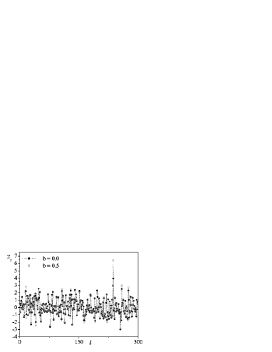
FIG. 1.: Two examples of ARCH time series obtained for a Gaussian noise (i.e., $q_{n}=1$). Memory (i.e., $b>0$) increases the probability for large values of $|z_{t}|$, i.e., fat tails in $P(z)$. The large value at $t=237$ is virtually never observed for $b=0$.

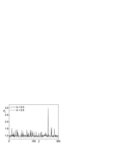
FIG. 2.: Time dependence of the volatility $\sigma$ for the same two ARCH processes shown in Fig. 1. The largest value for $\sigma$ occurs at $t=238$.

We shall now establish a possible analytical connection between the memory parameter $b$, $P\left(z\right)$ and $P_{n}\left(\omega\right)$ under the framework of the nonextensive statistical mechanics introduced by one of us [13]. Consider a probability distribution $P^{\prime}\left(z\right)$ such that it maximizes the entropic form

$$S_{q}=\frac{1-\int_{-\infty}^{+\infty}\left[P^{\prime}(z)\right]^{q}dz}{q-1}\;\;\;\;(q\in\ \Re)\,,$$ (6)

with $\lim_{q\to 1}S_{q}=-\int_{-\infty}^{+\infty}P^{\prime}(z)\ln P^{\prime}(z)dz\equiv S_{BG}$ ($BG$ stands for Boltzmann-Gibbs). Maximizing Eq. (6) with the constraints $\int_{-\infty}^{+\infty}P^{\prime}(z)dz=1$ and$\ \int_{-\infty}^{+\infty}z^{2}P^{\prime}(z)dz=1$ we have

$$P^{\prime}(z)=\frac{{\cal A}}{[1+{\cal B}(q-1)z^{2}]^{\frac{1}{q-1}}}\;\;\;\;(q<5/3)\,,$$ (7)

with

$${\cal B}\equiv\frac{\Gamma\left[\frac{5-3q}{2q-2}\right]}{2(q-1)\Gamma\left[\frac{3-q}{2q-2}\right]}\,,$$ (8)

and

$${\cal A}\equiv\frac{\Gamma\left[\frac{1}{q-1}\right]}{\sqrt{2\pi}\Gamma\left[\frac{3-q}{2q-2}\right]}\sqrt{(2q-1){\cal B}}\,.$$ (9)

In the $q\rightarrow 1$ limit, the normal distribution is recovered. The fourth moment (which for this case coincides with the kurtosis) is given by,

$$\left\langle z^{4}\right\rangle=3\frac{\Gamma\left[\frac{7-5q}{2q-2}\right]\Gamma\left[\frac{3-q}{2q-2}\right]}{\left\{\Gamma\left[\frac{5-3q}{2q-2}\right]\right\}^{2}}\;\;\;\;(1<q<\frac{7}{5})\;.$$ (10)

Let us now make the ansatz $P^{\prime}\left(z\right)\simeq$ $P\left(z\right)$. Consistently we impose the matching of Eqs. (5) and (10) . This yields $q$ as a function of $b$ and $k_{\omega}$. Assuming that noise $\omega_{t}$ follows a generalized distribution, Eq. (7), defined by an entropic index $q_{n}$ (such that $k_{w}^{(q_{n})}b^{2}<1$) we are able to establish a relation between the memory parameter $b$ and the entropic indexes $q$ and $q_{n}$, which characterize respectively the distributions $P^{\prime}\left(z\right)$ and $P_{n}\left(w\right)$. This connection is straightforwardly given by

$$b=\frac{\sqrt{G(q)\left\{\Gamma\left[\frac{5-3q_{n}}{2q_{n}-2}\right]\right\}^{2}-G(q_{n})\left\{\Gamma\left[\frac{5-3q}{2q-2}\right]\right\}^{2}}}{\sqrt{G(q_{n})\left(3G(q)-\left\{\Gamma\left[\frac{5-3q}{2q-2}\right]\right\}^{2}\right)}}\,,$$ (11)

where $G(x)\equiv\Gamma\left[\frac{7-5x}{2x-2}\right]\Gamma\left[\frac{3-x}{2x-2}\right]$. This connection, depicted in Fig. 3, constitutes, to the best of our knowledge, the first ever found which analytically expresses the return distribution in terms of the noise distribution and the memory parameter $b$. In what follows we shall verify that the above ansatz is indeed satisfied within a remarkable precision. To do this for typical values of $b$ and $q_{n}$, we first generate, through a standard algorithm based on Eq.(1) (with $s=1$), a set of ARCH time series and their corresponding probability density functions (PDF’s) $P(z)$. The results are indicated in Figs. 4 and 5. Then we compare with a histogram (with a conveniently chosen unit interval $\delta$) associated with the distribution (7), with $q$ satisfying Eq. (11). In other words, we compare with ${\cal A}_{\delta}\left[1-{\cal B}\left(1-q\right)x^{2}\right]^{\frac{1}{1-q}}$, where ${\cal B}$ is given by Eq. (8), and

$$\begin{array}[]{c}{\mathcal{A}}_{\delta}=\int_{-\delta/2}^{+\delta/2}p(z)dz=\frac{\delta}{\sqrt{2\pi}}\frac{\Gamma\left[\frac{1}{q-1}\right]}{\Gamma\left[\frac{3-q}{2q-2}\right]}\sqrt{\frac{\Gamma\left[\frac{5-3q}{2q-2}\right]}{\Gamma\left[\frac{3-q}{2q-2}\right]}}\\ \times\,_{2}F_{1}\left(\frac{1}{2},\frac{1}{q-1};\frac{3}{2},-\frac{\delta^{2}\Gamma\left[\frac{5-3q}{2q-2}\right]}{8\Gamma\left[\frac{3-q}{2q-2}\right]}\right)\end{array}$$ (12)

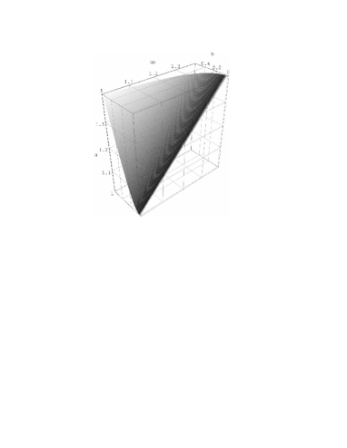
FIG. 3.: Diagram $(q,q_{n},b)$ for the ARCH process with $\left\langle z^{2}\right\rangle=1$ (for $b=0$ we have the straight line $q=q_{n}$).

We verify that the agreement is quite satisfactory. In order to quantify the small discrepancy between the ARCH PDF’s $P(z)$ and the analytical ones $P^{\prime}(z)$, we have indicated in the captions of Figs. 4 and 5 the values of $\chi^{2}\equiv\frac{1}{N}\,\sum\limits_{i=1}^{N}[P(z_{i})-P^{\prime}(z_{i})]^{2}$, $N$ being the number of points. An alternative evaluation of the discrepancy of the ARCH and analytical distribution can be done by comparing the sixth-order moment. It is simple to verify that these momenta for $P(z)$ and $P^{\prime}(z)$ exhibit quite small discrepancies. For example, for the cases illustrated in Figs. 4 and 5, we have obtained discrepancies never larger than $2.9\%$ (occuring in fact for $b\simeq 0.5$) for $q_{n}=1$ and than $2.7\%$ (occuring in fact for $b\simeq 0.3$) for $q_{n}=1.3$. Such minor discrepancies are, in financial practice, completely inocuous (for example, we may check in [14, 15] that realistic return distributions are larger than $10^{-6}$, whereas in our present Figs. 4 and 5 we have simulated down to $10^{-8}$).

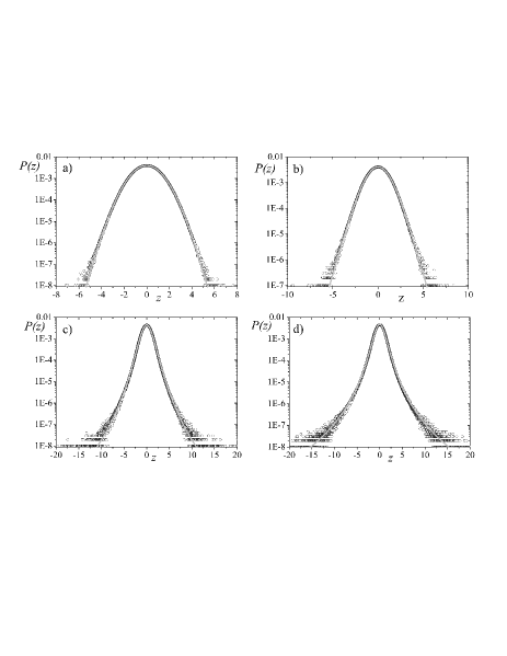
FIG. 4.: PDFs for a $q_{n}=1$ noise and typical values of $b$. a) $b=0$, $q=1$ ($\chi^{2}=1.14\times 10^{-11}$); b) $b=0.1$, $q=1.01976$ ($\chi^{2}=2.34\times 10^{-10}$); c) $b=0.4$, $q=1.242424$ ($\chi^{2}=1.82\times 10^{-10}$); d) $b=0.5$, $q=\frac{4}{3}$ ($\chi^{2}=2.98\times 10^{-10}$).

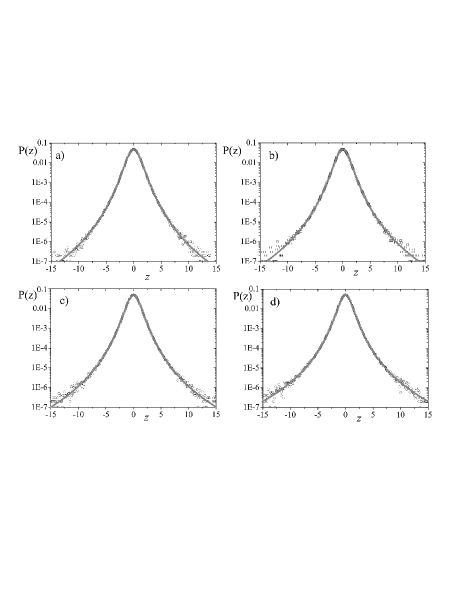
FIG. 5.: PDFs for a $q_{n}=1.3$ noise and typical values of $b$. a) $b=0$, $q=1.3$ ($\chi^{2}=3.93\times 10^{-10}$); b) $b=0.1$, $q=1.30762$ ($\chi^{2}=8.86\times 10^{-10}$); c) $b=0.2$, $q=1.32950$ ($\chi^{2}=9.72\times 10^{-10}$); d) $b=0.3$, $q=1.36306$ ($\chi^{2}=2.68\times 10^{-10}$).

Let us conclude by saying that the fact that a close connection has been shown to exist between the possibly ubiquitous ARCH stochastic processes and the nonextensive entropy Eq.(6) strongly suggests further possible connections. We refer to phenomena which might present some kind of scale invariant geometry, e.g., hierarchical or multifractal structures, low-dimensional dissipative and conservative maps [16], fractional and/or nonlinear Fokker-Planck equations [17], Langevin dynamics with fluctuating temperature [18], possibly scale-free network growth [19], long-range many-body classical Hamiltonians [20, 21, 22], among others. A more detailed study of this as well as of other heteroskedastic models (e.g., GARCH) is in progress.

We acknowledge useful remarks from J.D. Farmer, as well as partial support from Faperj, CNPq, PRONEX/MCT (Brazilian agencies) and FCT/MCES (contract SFRH/BD/6127/2001) (Portuguese agency).

REFERENCES

- [1] B.M. Mandelbrot, J. Business 36, 394 (1963).
- [2] E.F. Fama, J. Business 38, 34 (1965).
- [3] J.-Ph. Bouchaud and M. Potters, Theory of Financial Risks: From Statistical Physics to Risk Management (Cambridge University Press, Cambridge, 2000); R.N. Mantegna and H.E. Stanley, An Introduction to Econophysics: Correlations and Complexity in Finance (Cambridge University Press, Cambridge, 1999).
- [4] R.F. Engle, Econometrica 50, 987 (1982).
- [5] T. Bollerslev R.Y. Chou and K.F. Kroner, J. Econometrics 52, 5 (1992).
- [6] S.H. Poon and C.W.J. Granger, J. Econ. Lit. 41, 478 (2003).
- [7] T.H. McCurdy and T. Stengos, J. Econometrics 52, 225 (1992).
- [8] I. Zovko and J. Doyne Farmer, Quantitative Finance 2, 387 (2002).
- [9] H. White, Econometrica 50, 1 (1982).
- [10] A.A. Weiss, Journal of Time Series Analysis 5, 129 (1984).
- [11] T. Bollerslev, Rev. Econ. Stat. 69, 542 (1987).
- [12] B. Podobnik, P.Ch. Ivanov, Y. Lee, A. Cheesa and H.E. Stanley , Europhys. Lett. 50, 711 (2000)
- [13] C. Tsallis, J. Stat. Phys. 52, 479 (1988). A regularly updated bibliography on the subject is avaible at http://tsallis.cat.cbpf.br/biblio.htm.
- [14] R. Osorio, L. Borland and C. Tsallis, in Nonextensive Entropy - Interdisciplinary Applications, eds. M. Gell-Mann and C. Tsallis (Oxford University Press, New York, 2004), in press.
- [15] L. Borland, Phys. Rev. Lett. 89, 098701 (2002); L. Borland, Quantitative Finance 2, 415 (2002).
- [16] M.L. Lyra and C. Tsallis, Phys. Rev. Lett. 80, 53 (1998); F. Baldovin and A. Robledo, Europhys. Lett. 60, 518 (2000).
- [17] L. Borland, Phys. Rev. E 57, 6634 (1998).
- [18] C. Beck and E.G. Cohen, Physica A 322, 267 (2003).
- [19] R. Albert and A.L. Barabasi, Phys. Rev. Lett. 85, 5234 (2000).
- [20] V. Latora, A. Rapisarda and C. Tsallis, Phys. Rev. E 64, 056134 (2001).
- [21] S. Abe and Y. Okamoto, eds., Nonextensive Statistical Mechanics and Its Applications (Springer-Verlag, Berlin, 2001)
- [22] M. Gell-Mann and C. Tsallis, eds., Nonextensive Entropy – Interdisciplinary Applications (Oxford University Press, New York, 2004), in press.