Nonequilibrium Transport through a Kondo Dot:
Decoherence Effects.

Abstract

We investigate the effects of voltage induced spin-relaxation in a quantum dot in the Kondo regime. Using nonequilibrium perturbation theory, we determine the joint effect of self-energy and vertex corrections to the conduction electron T-matrix in the limit of transport voltage much larger than temperature. The logarithmic divergences, developing near the different chemical potentials of the leads, are found to be cut off by spin-relaxation rates, implying that the nonequilibrium Kondo-problem remains at weak coupling as long as voltage is much larger than the Kondo temperature.

Electron transport through quantum dots or point contacts possessing a degenerate ground state (e.g. a spin) is strongly influenced by the Kondo effect Hewson93 , provided the dot is in the Coulomb blockade regime. In the linear response regime, the Kondo resonance formed at the dot at sufficiently low temperature, i.e. at or below the Kondo temperature $T_{K}$, allows for resonant tunneling, thus removing the Coulomb blockade and leading to conductances near the unitarity limit. This has been observed in various experiments on quantum dot devices Experiments .

The Kondo resonance is quenched by either large temperature, $T\gg T_{K}$, large magnetic field, $B\gg T_{K}$ or a large bias voltage, $V\gg T_{K}$. However, the mechanism of how and why the Kondo effect is suppressed is qualitatively different in the three cases. The Kondo effect arises from resonant spin-flip scattering at the Fermi energy. Temperature destroys the resonance mainly by smearing out the Fermi surface, whereas a magnetic field lifts the degeneracy of the levels on the dot and thereby prohibits resonant scattering. The effect of a bias voltage, $V$, is more subtle. It induces a splitting of the Fermi energies of the left, and the right lead. However, this splitting affects directly only resonant electron scattering from the left to the right lead, but not any scattering which begins and ends on the same lead. Yet these remaining resonant processes are suppressed by a different effect: the voltage induces a current which leads to noise and therefore to decoherence of resonant spin-flips. It is the goal of this paper to study those decoherence effects in detail.

In perturbation theory, the signature of Kondo physics are logarithmic divergences arising from (principle value) integrals of the type

$$\int_{-D}^{D}\!d\omega\,\frac{f(\omega)}{\omega}\sim\ln\frac{D}{E_{\rm{IR}}}$$ (1)

where $f(\omega)$ is the Fermi function, $D$ a high energy cutoff (i.e. bandwidth) and $E_{\rm{IR}}$ some infrared cutoff. There are three rather different ways to cut off the logarithm, and to destroy the Kondo effect, corresponding to the three mechanisms discussed above. First, temperature broadens $f(\omega)$ leading to $E_{\rm{IR}}\sim T$. Second, a magnetic field $B$ shifts the pole with respect to the Fermi-energy, replacing $\frac{1}{\omega}$ by $\frac{1}{\omega-B}$, and in this case $E_{\rm{IR}}\sim B$. The third way to quench the logarithm is to introduce a finite decoherence rate $\Gamma_{\!s}$, replacing $\frac{1}{\omega}$ by $\frac{\omega}{\omega^{2}+\Gamma_{\!s}^{2}}$, implying $E_{\rm{IR}}\sim\Gamma_{\!s}$.

The relaxation rate $\Gamma_{\!s}=\Gamma_{\!s}(V,B,T)$ and the associated decoherence effects also exist in equilibrium. In the limit of vanishing bias voltage and magnetic field, the scale $\Gamma_{\!s}$ tends to a temperature dependent (Korringa) rateKorringa50 , $\Gamma_{\!s}(0,0,T)\ll T$, which vanishes as $T\to 0$, allowing for the quantum coherent Kondo state to be formed. In the case of a finite magnetic field and zero temperature, a $B$- and spin-dependent rateWang68 , $\Gamma_{\!s,\sigma}(0,B,0)$ remains finite for the excited state $\sigma=\downarrow$. In dynamic quantities it prohibits singular behavior at $\omega\sim B$ but it is not important for static quantities, where $B$ eliminates all relevant singularities. In the case of a finite bias voltage $V$, however, the finite rate $\Gamma_{\!s}(V,0,0)$ is instrumental to cut off singularities even in static quantities for $T,B\to 0$. The Kondo effect develops only to a certain extent, depending on the ratio $V/T_{K}$.

Not only for a quantitative description of experiments in the regime $V\gg T_{K}$, but even for a crude qualitative understanding of Kondo physics out of equilibrium, it is necessary to identify the correct relaxation rate $\Gamma_{\!s}$. The question, how logarithmic contributions are cut off, is essential to derive the correct perturbative renormalization group descriptionSchoeller00 ; Rosch03a and to identify regimes where novel strong-coupling physics is induced out of equilibrium.

The importance of the broadening of the Zeeman levels was pointed out three decades ago by Wolf and LoseeWolf69 in the context of the Kondoesque tunneling anomaly observed in various tunnel junctions. Incorporating a Korringa like, $T$ and $B$ dependent, spin-relaxation rate into Appelbaum’s perturbative formula for the conductanceAppelbaum66 was found to improve the agreement with experiments considerably (cf. e.g. Refs. Appelbaum72, and Bermon78, ). Later, in the context of quantum dots, Meir et al.Meir93 pointed out that, even at $T=B=0$, the finite bias-voltage induces a broadening of the Zeeman levels. In their self-consistent treatment of the Anderson model, using the non-crossing approximation (NCA), this nonequilibrium broadening was shown to suppress the Kondo peaks in the local density of states, located at the two different Fermi levels. In Ref. Rosch01, we showed that this NCA relaxation rate is sufficiently large to prohibit the flow towards strong coupling for $V\gg T_{K}$. In a perturbative study of the effects of an ac-bias, Kaminski et al.Kaminski99 argued that an irradiation induced broadening serves to cut off the logarithmic divergence of the conductance as $T$ and $V$ tend to zero. Treatments of the Kondo modelColeman01 and related problemsKiselev02 at large voltages, which neglect the influence of decoherence, find strong coupling effects even for $V\gg T_{K}$. Coleman et al.Coleman01 recently argued that this is the case because $\Gamma_{\!s}$ remains sufficiently small due to a (supposed) cancellation of vertex and self-energy corrections.

To our knowledge, even to lowest order in perturbation theory, a systematic calculation of the nonequilibrium decoherence rate is still lacking. It is the objective of this paper to provide such a calculation. This is a delicate matter since self-energy, and vertex corrections may indeed cancel partially, and an infinite resummation of perturbation theory is required. RecentlyMao03 ; Shnirman03 , it was demonstrated that the Majorana fermion representation for the local spin-$1/2$ circumvents this complication when calculating spin-spin correlation functions. In this representation, such correlators take the form of one-particle, rather than two-particle, fermionic correlation functions, and consequently only self-energy corrections have to be considered. Whether this representation will prove to be equally efficient for calculating other observables like the conduction electron T-matrix or the conductance remains to be seen.

Based on the conjecture that no unexpected cancellations occur, we have recently developed a perturbative renormalization group descriptionRosch03a of the Kondo effect at large voltages. In this approach, it was essential to include the effects of $\Gamma_{\!s}$. For usual quantum dots, the Kondo effect is sufficiently suppressed by $\Gamma_{\!s}$Rosch01 ; Rosch03a , such that renormalized perturbation theory remains applicable at all temperatures, provided $\ln(V/T_{K})\gg 1$. We argued that $\Gamma_{\!s}$, as a physically observable quantity, should be identified with the transverse spin relaxation rate $\Gamma_{2}=1/T_{2}$, measuring the coherence property of the local spin (More precisely, slightly different rates enter into various physical quantities, but to leading order in $1/\ln[V/T_{K}]$ one can use $\Gamma_{\!s}\approx\Gamma_{2}$). In this paper we show that within perturbation theory this is indeed the case, thus confirming our initial conjecture. Note that in more complex situations, for example in the case of coupled quantum dots, $\Gamma_{\!s}$ can be sufficiently smallRosch01 so that novel (strong coupling) physics can be induced for large voltages.

In a preceding paperPaaske03a , henceforth referred to as I, we calculated perturbatively the local magnetization and the differential conductance of a Kondo dot, including all leading logarithmic corrections in the presence of finite $V$ and $B$. As effects of $\Gamma_{\!s}$ are not included to this order, some logarithms were not cut off by $V$ but appeared to diverge with $\ln(D/T)$ or $\ln(D/|V-B|)$. A systematic calculation of the cut-off $\Gamma_{\!s}$ requires a consistent resummation of self-energy and vertex corrections. As will become clear in the following, this is a formidable task, and we have therefore concentrated on the quantity which appears to be most tractable: the conduction electron T-matrix as a function of frequency, in zero magnetic field.

In Sec. I we introduce the model and some conventions used for the Keldysh perturbation theory. A combination of self-energy corrections from Sec. II.1 and vertex-corrections calculated in Sec. II.2 determines the spin-relaxation rate (Sec. II.3). In Sec. III we show how this decoherence rate cuts off logarithmic corrections in the T-matrix. In Sec. IV we consider the case of anisotropic exchange couplings and determine the exact combination of transverse and longitudinal spin-relaxation rates which enters the logarithms in the T-matrix. Appendices A and B contain details pertaining to Sections II.2 and III. Appendix C investigates how power-law singularities of the strongly anisotropic Kondo model are modified out of equilibrium by mapping it to the nonequilibrium X-ray edge problem for vanishing spin-flip coupling.

I Model and Method

We model the quantum dot by its local spin $\vec{S}$ $(S=\frac{1}{2})$, coupled by the exchange interaction $J_{\alpha\alpha^{\prime}}$ ($\alpha,\alpha^{\prime}=L,R$) to the conduction electrons in the left (L) and right (R) leads

$$H = \sum_{\alpha,{\bf k},\sigma}(\varepsilon_{{\bf k}}-\mu_{\alpha})c^{\dagger}_{\alpha{\bf k}\sigma}c_{\alpha{\bf k}\sigma}-g\mu_{B}BS_{z}$$ (2)

$$+\!\sum_{\alpha,\alpha^{\prime},{\bf k},{\bf k}^{\prime},\sigma,\sigma^{\prime}}\!\!\!\!\!J_{\alpha^{\prime}\alpha}\,\vec{S}\cdot\frac{1}{2}\,c^{\dagger}_{\alpha^{\prime}{\bf k}^{\prime}\sigma^{\prime}}\vec{\tau}_{\sigma^{\prime}\sigma}c_{\alpha{\bf k}\sigma},$$

where $J_{LR}$ describes a co-tunneling process transferring an electron from the right to the left lead. Here $\mu_{L,R}=\pm eV/2$ are the chemical potentials of respectively the left and right leads, $\vec{\tau}$ is the vector of Pauli matrices, $g\mu_{B}B$ the Zeeman splitting of the local spin levels in a magnetic field $B$, and $c_{\alpha{\bf k}\sigma}^{\dagger}$ creates an electron in lead $\alpha$ with momentum ${\bf k}$ and spin $\sigma$. We will use dimensionless coupling constants $g_{\alpha\alpha^{\prime}}=N(0)J_{\alpha\alpha^{\prime}}$, with $N(0)$ the density of states per spin for the conduction electrons (assumed flat on the scale $eV,g\mu_{B}B$). We define for later use $g_{d}=(g_{LL}+g_{RR})/2$, $4g^{2}=g_{LL}^{2}+g_{RR}^{2}+2g_{LR}^{2}$ and use units where $\hbar=k_{B}=g\mu_{B}=e=1$.

In order to calculate observable quantities for the system with Hamiltonian (2), we find it convenient to use a fermionic representation of the local spin operator,

$$\vec{S}=\frac{1}{2}\sum_{\gamma\gamma{{}^{\prime}}}f_{\gamma}^{\dagger}\vec{\tau}_{\gamma\gamma{{}^{\prime}}}f_{\gamma{{}^{\prime}}},$$ (3)

with canonical fermion creation and annihilation operators $f_{\gamma}^{\dagger}$, $f_{\gamma}$, $\gamma=\uparrow\downarrow$, which allows a conventional diagrammatic perturbation theory in the coupling constant $g$. Since the physical Hilbert space must have singly occupied states only, it is necessary to project out the empty and doubly occupied local states. This is done by introducing a chemical potential $\lambda$ regulating the charge $Q=\sum_{\gamma}f_{\gamma}^{\dagger}f_{\gamma}$. Picking out the contribution proportional to $e^{-\beta\lambda}$ and taking the limit $\lambda\to\infty$, the constraint $Q=1$ can be enforced (for a more detailed description of this method see I).

We will use the Keldysh Green function method for nonequilibrium systems, following the notation of Ref. Rammer86, . Keldysh matrix propagators are defined as

$$\underline{G}=\left(\begin{array}[]{cc}G^{R}&G^{K}\\ 0&G^{A}\\ \end{array}\right)$$ (6)

where $G^{R,A}$ and $G^{K}$ are the retarded, advanced and Keldysh component Green functions, respectively. Spectral functions are found as $A=i(G^{R}-G^{A})$, and the greater and lesser functions as

$$G^{>/<}=(G^{K}\pm G^{R}\mp G^{A})/2.$$ (7)

The local conduction electron ($ce$) Green functions at the dot in the left and right leads, and the pseudo fermion ($pf$) Green function are denoted by $G_{\alpha\sigma}^{ab}$ and ${\cal G}_{\gamma}^{cd}$, respectively, with lead index $\alpha=L,R$, spin indices $\sigma,\gamma$, and Keldysh indices $a,b,c,d$. A corresponding notation will be used for the self-energy $\Sigma$, and its imaginary part, the self-energy broadening, is denoted by $\Gamma_{\gamma}=i(\Sigma^{R}_{\gamma}-\Sigma^{A}_{\gamma})$. The interaction vertex has the following tensor structure in Keldysh space

$$\Lambda_{ab}^{cd}=\frac{1}{2}\left(\delta_{ab}\tau^{1}_{cd}+\tau^{1}_{ab}\delta_{cd}\right),$$ (8)

where $a,b$ and $c,d$ refer to $pf$, and $ce$-lines, respectively.

Since we consider only nonequilibrium situations in a steady state, time translation invariance holds, and the single-particle Green functions depend only on one frequency. The bare $pf$ spectral function is given by

$${\cal A}_{\gamma}(\omega)=2\pi\delta(\omega+\gamma B/2),$$ (9)

and the Keldysh component Green function is given as

$${\cal G}^{K}_{\gamma}(\omega)=i{\cal A}_{\gamma}(\omega)[2n_{\gamma\lambda}(\omega)-1],$$ (10)

where $n_{\gamma\lambda}(\omega)$ denotes the $pf$ distribution function, given by $n_{\gamma\lambda}(\omega)=1/(e^{(\omega+\lambda)/T}+1)$ in thermal equilibrium. We shall also use the shorthand notation

$$M_{\gamma\lambda}=2n_{\gamma\lambda}(\omega)-1.$$ (11)

Assuming a constant conduction electron density of states $N(0)=1/2D$ and a bandwidth $2D$, the local $ce$ spectral function takes the form

$$A(\omega)=2\pi N(0)\theta(D-|\omega|)$$ (12)

with the step function $\theta(x)$. The Keldysh component Green function in lead $\alpha$ is then given by

$$G^{K}_{\alpha}(\omega)=-iA(\omega)\tanh\left(\frac{\omega-\mu_{\alpha}}{2T}\right),$$ (13)

assuming the electrons in each lead to be in thermal equilibrium.

II Spin level broadening and spin relaxation rates

The coupling of the local spin to the leads introduces a broadening of the Zeeman levels, which depends on temperature, magnetic field and bias voltage. In the pseudo fermion representation for the local spin, the broadening is given by the imaginary part of the pseudo fermion self-energy. This level broadening enters into the relaxation rates of both the transverse spin components $(S_{x},S_{y})$, where it accounts for the loss of phase coherence, and the longitudinal spin component $(S_{z})$, where it describes the relaxation of the local magnetization following a change in the magnetic field. The observable spin relaxation rates, $1/T_{2}$ and $1/T_{1}$, are defined through the broadening of the resonance poles in the transverse, and longitudinal dynamical spin susceptibilities, and their calculation requires vertex corrections to be included in a consistent way.

Following a brief discussion of the $pf$ self-energy broadening, we determine the renormalized $ce$-$pf$ interaction vertex in a steady-state nonequilibrium situation. The resulting vertex functions are used to calculate the transverse dynamical spin susceptibility, and later, in Sec. III, they will serve as building blocks for a calculation of the conduction electron T-matrix.

II.1 Pseudo Fermion Decay Rates

In paper I (Ref. Paaske03a, ), we determined the on-shell imaginary part of the pseudo fermion self-energy, including leading logarithmic corrections. For the purpose of this paper, we will only need the second order rates, disregarding logarithmic corrections. For $T=0$ one finds for $0\leq V<B$:

$$\Gamma_{\uparrow} = \frac{\pi}{4}g_{LR}^{2}V,$$ (14)

$$\Gamma_{\downarrow} = \Gamma_{\uparrow}+2\pi g^{2}B,$$ (15)

with $4g^{2}=g_{LL}^{2}+g_{RR}^{2}+2g_{LR}^{2}$, whereas for $V>B\geq 0$:

$$\Gamma_{\uparrow} = \frac{\pi}{4}g_{LR}^{2}(3V-2B),$$ (16)

$$\Gamma_{\downarrow} = \Gamma_{\uparrow}+2\pi g^{2}B.$$ (17)

Notice that in the presence of a finite magnetic field, only the upper spin-level, here corresponding to spin down, is broadened when $V=0$, as one would expect from simple phase-space considerations. Broadening of the lower spin-level (spin up) is due to virtual transitions to the upper spin-level and occurs only in higher orders in $g$.

For comparison, we list also the thermal decay rate for $V=B=0$:

$$\Gamma_{\uparrow,\downarrow}=3\pi Tg^{2}.$$ (18)

II.2 Vertex Corrections

Early work Walker68 ; Woelfle71 ; Langreth72 on the dynamical magnetic susceptibility of a single spin 1/2, demonstrated how self-energy, and vertex corrections combine to yield the transverse, and longitudinal relaxation rates $1/T_{2}$ and $1/T_{1}$. In Ref. Walker68, , the vertex corrections were determined in the approximation where the imaginary part of the $pf$ self-energy, $\Gamma$, is much smaller than temperature. A similar approach is possible out of equilibrium, where it is the finite voltage, rather than temperature, which determines the abundance of (inter-lead) conduction electron particle-hole excitations. In the approximation where $\Gamma\ll V$, the dominant corrections to the $ce$-$pf$ interaction vertex (Keldysh) tensor simplify substantially and the corresponding vertex matrix equation can be solved analytically. Since we assume that $V\gg T_{K}$, perturbation theory is valid and $\Gamma\sim g^{2}V\ll V$ is indeed a sound approximation. We shall consider the case where $T\ll V$, which will best reveal the salient nonequilibrium features of the problem.

To calculate vertex corrections and their interplay with self-energy diagrams, we have to solve the vertex equation depicted in Fig. 1. We remind the reader that physical quantities are proportional to $e^{-\beta\lambda}$ within our projection scheme. Therefore we have to keep track of two contributions to the vertex

$${\tilde{\Lambda}}{{}_{ab}}\!\!\!\!\!{{}^{cd}}=^{0\!\!}{\tilde{\Lambda}}{{}_{ab}}\!\!\!\!\!{{}^{cd}}+^{\lambda\!\!}{\tilde{\Lambda}}{{}_{ab}}\!\!\!\!\!{{}^{cd}},$$ (19)

where ${}^{0\!}{\tilde{\Lambda}}$ is independent of $\lambda$, and ${}^{\lambda\!}{\tilde{\Lambda}}$ vanishes as $e^{-\beta\lambda}$ in the limit of $\lambda\to\infty$. We shall first determine ${}^{0\!}{\tilde{\Lambda}}$ and then, in a second step, ${}^{\lambda\!}{\tilde{\Lambda}}$.

II.2.1 Voltage induced Particle-Hole Excitations

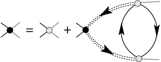
Figure 1: Vertex equation for the $pf-ce$ vertex, including only non-logarithmic irreducible parts.

We start by discussing the properties of the $ce$ polarization bubble in Keldysh space, which enters as one building block in the vertex equation shown in Fig. 1. The convolution of two conduction electron Green functions has the greater component

$${{}_{\alpha\!}}\!\!\!\!{{}^{\alpha^{\prime}\!}}\Pi{{}_{\,\,\,}}\!\!\!\!\!{{}^{\,\,\,>}}(\Omega)=\!\int\!\frac{d\varepsilon}{2\pi}G^{>}_{\alpha^{\prime}}(\varepsilon+\Omega)G^{<}_{\alpha}(\varepsilon),$$ (20)

and in general, the convolution of different Keldysh-components gives rise to the polarization tensor

$${{}_{\alpha\!}}\!\!\!\!{{}^{\alpha^{\prime}\!}}\Pi{{}_{dc}}\!\!\!\!\!{{}^{d^{\prime}\!c^{\prime}}}(\Omega)=\!\int\!\frac{d\varepsilon}{2\pi}\underline{G}^{d^{\prime}\!c^{\prime}}_{\alpha^{\prime}}\!(\varepsilon+\Omega)\underline{G}^{dc}_{\alpha}(\varepsilon).$$ (21)

It is convenient to form the contraction of this tensor with the exchange constants $J_{\alpha\alpha^{\prime}}/4$ at each end, and thus define an effective second order interaction by

$${}\!\!\!\!{}\Pi{{}_{dc}}\!\!\!\!\!{{}^{d^{\prime}\!c^{\prime}}}(\Omega)\equiv\frac{1}{16}J^{2}_{\alpha\alpha^{\prime}}{{}_{\alpha\!}}\!\!\!\!{{}^{\alpha^{\prime}\!}}\Pi{{}_{dc}}\!\!\!\!\!{{}^{d^{\prime}\!c^{\prime}}}(\Omega).$$ (22)

Contracting again this $ce$ polarization tensor with two bare Keldysh vertices yields the $pf$ interaction tensor

$$B{{}_{b^{\prime}a}}\!\!\!\!\!{{}^{a^{\prime}b}} = \Lambda{{}_{a^{\prime}b}}\!\!\!\!\!{{}^{\!c^{\prime}d}}\Pi{{}_{dc}}\!\!\!\!\!{{}^{d^{\prime}\!c^{\prime}}}\!\Lambda{{}_{ab^{\prime}}}\!\!\!\!\!{{}^{\!cd^{\prime}}}$$

$$= \frac{1}{2}\left\{\Pi^{K}\delta_{a^{\prime}b}\delta_{ab^{\prime}}+\Pi^{A}\delta_{a^{\prime}b}\tau^{1}_{ab^{\prime}}+\Pi^{R}\tau^{1}_{a^{\prime}b}\delta_{ab^{\prime}}\right\},$$

where the Langreth rules (cf. Ref. Langreth76, ) have been employed to work out the contractions

$$\Pi{{}_{dc}}\!\!\!\!\!{{}^{{\overline{c}}{\overline{d}}}}=2\Pi^{K},\,\,\,\,\,\,\Pi{{}_{dc}}\!\!\!\!\!{{}^{c{\overline{d}}}}=2\Pi^{A},\,\,\,\,\,\,\Pi{{}_{dc}}\!\!\!\!\!{{}^{{\overline{c}}d}}=2\Pi^{R},$$ (24)

using the notation ${\overline{1}}=2$ and ${\overline{2}}=1$ for the Keldysh indices. As for the single particle Green functions, we organize these components in a triangular matrix

$$\underline{\Pi}=\left(\begin{array}[]{ll}\Pi^{R}&\Pi^{K}\\ 0&\Pi^{A}\end{array}\right),$$ (25)

and for $\Omega\ll D$ one finds that

$$\Pi^{R/A}(\Omega)\!=\!\frac{\pi}{16}g^{2}_{\alpha\alpha^{\prime}}\left\{\pm(\Omega+\mu_{\alpha}-\mu_{\alpha^{\prime}})-i\frac{4D\ln 2}{\pi}\right\},\\ \Pi^{K}(\Omega)\!=\!\frac{\pi}{8}g^{2}_{\alpha\alpha^{\prime}}(\Omega+\mu_{\alpha}-\mu_{\alpha^{\prime}})\coth\left(\frac{\Omega+\mu_{\alpha}-\mu_{\alpha^{\prime}}}{2T}\right).$$ (26)

Notice that inter-lead particle-hole excitations do not satisfy the fluctuation-dissipation theorem as

$${{}_{\alpha\!}}\!\!\!\!{{}^{\alpha^{\prime}\!}}\Pi{{}_{\,\,\,}}\!\!\!\!\!{{}^{\,\,\,K}}(\Omega)=\coth\left(\frac{\Omega+\mu_{\alpha}-\mu_{\alpha^{\prime}}}{2T}\right)\!\left[\,{{}_{\alpha\!}}\!\!\!\!{{}^{\alpha^{\prime}\!}}\Pi{{}_{\,\,\,}}\!\!\!\!\!{{}^{\,\,\,R}}(\Omega)-{{}_{\alpha\!}}\!\!\!\!{{}^{\alpha^{\prime}\!}}\Pi{{}_{\,\,\,}}\!\!\!\!\!{{}^{\,\,\,A}}(\Omega)\right].$$

The lead-contracted polarization satisfies the following symmetries:

$$\Pi^{>/K/R/A}(-\Omega)=\Pi^{</K/A/R}(\Omega),$$ (27)

and for later use we quote the explicit formula for the ${\it greater}$ component, $\Pi^{>}=(\Pi^{K}+\Pi^{R}-\Pi^{A})/2$:

$$\Pi^{>}(\Omega)=\frac{\pi}{8}\left\{g_{LR}^{2}\left[(\Omega+V)(1+N(\Omega+V))\right.\right.$$

$$\left.\left.+(\Omega-V)(1+N(\Omega-V))\right]+2g_{d}^{2}\Omega(1+N(\Omega))\right\},$$

where $N(\Omega)$ denotes the Bose-function and $\Pi^{>}(\Omega)=0$ for $\Omega\geq 2D+V$. In terms of this function, the second order $pf$ decay rate may be written as

$$\Gamma_{\gamma}(\omega)=2\theta_{\gamma\gamma^{\prime}}\Pi^{>}(-\omega-\gamma^{\prime}B/2),$$ (29)

with $\theta_{\gamma\gamma^{\prime}}=\delta_{\gamma\gamma^{\prime}}+2\tau_{\gamma\gamma^{\prime}}^{1}$.

II.2.2 Basic Approximations

The following calculations are based on self-consistent perturbation theory to order $g^{2}$ for self-energies and vertex corrections. As explained in detail in I, self-consistency is essential to obtain for example the correct magnetization out of equilibrium. For this paper, we need a self-consistent resummation of diagrams to investigate how divergences of bare perturbation theory are cut off to lowest order in the interactions.

However, for non-singular quantities like the lowest-order self-energy, self-consistency only gives rise to subleading corrections which we need not keep track of. For example, it is sufficient to approximate the retarded $pf$ propagators (double-dashed lines in the diagrams) by

$${\cal G}^{R}_{\gamma}(\omega)=\frac{1}{\omega+\gamma B/2+i\Gamma_{\gamma}/2},$$ (30)

where $\Gamma_{\gamma}$, given in Eqs. (14-17), denotes the on-shell decay rate calculated in bare perturbation theory. We neglect contributions from $\text{Re}\Sigma_{\gamma}(\omega)$ which can be absorbed in a redefinition of $B$ and $g$, and which give rise only to subleading corrections in the following.

To show, formally, that self-consistency does not change this result, one can use the fact that typical integrals are dominated by integrations over frequencies in a window of width $\Gamma$ around the Zeeman levels. Since the various Keldysh components of $\Pi$ vary slowly with frequency, i.e. $[\Pi(\omega+\Gamma)-\Pi(\omega)]/\Pi(\omega)\sim\Gamma/V$, we may therefore use $\Gamma/V\sim g^{2}$ as a small expansion parameter (this will be shown explicitly for the vertex corrections below).

II.2.3 Summing up the Ladder

To leading order in $\Gamma/V\sim g^{2}$, the renormalized vertex satisfies the diagrammatic equation depicted in Fig. 1. This equation generates a series of ladder diagrams with dressed $pf$-legs and bare $ce$ particle-hole propagators as rungs. Contributions from diagrams with crossed rungs we omit as being of order $\Gamma/V$. In appendix A, we establish this relative smallness explicitly for the crossed 4’th order vertex correction and we expect higher order corrections to work in the same way.

An iterative solution for the renormalized vertex starts with the attachment of two $pf$-propagators to the bare Keldysh vertex. This defines the tensor

$${{}_{\gamma^{\prime}}}\!\!\!\!{{}^{\gamma}}V{{}_{ab}}\!\!\!\!\!{{}^{cd}}=2\Lambda^{cd}_{a^{\prime}b^{\prime}}{\underline{\cal G}}^{b^{\prime}\!a}_{\gamma}{\underline{\cal G}}^{ba^{\prime}}_{\gamma^{\prime}},$$ (31)

which is found to have the following components:

$${{}_{\gamma^{\prime}}}\!\!\!\!{{}^{\gamma}}V{{}_{11}}\!\!\!\!\!{{}^{cd}} = \delta_{cd}\,{\cal G}^{R}_{\gamma}{\cal G}^{K}_{\gamma^{\prime}}+\tau^{1}_{cd}\,{\cal G}^{R}_{\gamma}{\cal G}^{R}_{\gamma^{\prime}},$$ (32)

$${{}_{\gamma^{\prime}}}\!\!\!\!{{}^{\gamma}}V{{}_{12}}\!\!\!\!\!{{}^{cd}} = \delta_{cd}\,{\cal G}^{R}_{\gamma}{\cal G}^{A}_{\gamma^{\prime}},$$ (33)

$${{}_{\gamma^{\prime}}}\!\!\!\!{{}^{\gamma}}V{{}_{21}}\!\!\!\!\!{{}^{cd}} = \delta_{cd}\left\{{\cal G}^{K}_{\gamma}{\cal G}^{K}_{\gamma^{\prime}}+{\cal G}^{A}_{\gamma}{\cal G}^{R}_{\gamma^{\prime}}\right\}$$ (34)

$$\!\!\!\!+\tau^{1}_{cd}\left\{{\cal G}^{K}_{\gamma}{\cal G}^{R}_{\gamma^{\prime}}+{\cal G}^{A}_{\gamma}{\cal G}^{K}_{\gamma^{\prime}}\right\},$$

$${{}_{\gamma^{\prime}}}\!\!\!\!{{}^{\gamma}}V{{}_{22}}\!\!\!\!\!{{}^{cd}} = \delta_{cd}\,{\cal G}^{K}_{\gamma}{\cal G}^{A}_{\gamma^{\prime}}+\tau^{1}_{cd}\,{\cal G}^{A}_{\gamma}{\cal G}^{A}_{\gamma^{\prime}}.$$ (35)

One proceeds by attaching rungs, using the interaction tensor $B{{}_{b^{\prime}\!a}}\!\!\!\!\!{{}^{a^{\prime}\!b}}$, and legs consisting of pairs of dressed $pf$ propagators. This attachment consists of a contraction of Keldysh, and spin indices, together with an integration over the frequency circulating the individual sections of the ladder. To leading order in $\Gamma/V$, we may perform these integrals by neglecting the slow frequency dependence of the $ce$ polarization functions compared to the rapid variations in the $pf$ Green functions. Making use of the identity

$$\frac{1}{a}\frac{1}{b}=\frac{1}{a-b}\left(\frac{1}{b}-\frac{1}{a}\right),$$ (36)

products of Green functions may be expressed as either

$${\cal G}^{R}_{\gamma}(\Omega+\omega){\cal G}^{A}_{\gamma^{\prime}}(\omega)=\frac{1}{\Omega+(\gamma-\gamma^{\prime})B/2+i(\Gamma_{\gamma}+\Gamma_{\gamma^{\prime}})/2}$$

$$\times\left(\frac{1}{\omega+\gamma^{\prime}B/2-i\Gamma_{\gamma^{\prime}}/2}-\frac{1}{\Omega+\omega+\gamma B/2+i\Gamma_{\gamma}/2}\right)$$

or

$${\cal G}^{R}_{\gamma}(\Omega+\omega){\cal G}^{R}_{\gamma^{\prime}}(\omega)=\frac{1}{\Omega+(\gamma-\gamma^{\prime})B/2+i(\Gamma_{\gamma}-\Gamma_{\gamma^{\prime}})/2}$$

$$\times\left(\frac{1}{\omega+\gamma^{\prime}B/2+i\Gamma_{\gamma^{\prime}}/2}-\frac{1}{\Omega+\omega+\gamma B/2+i\Gamma_{\gamma}/2}\right)$$

and likewise for $AR$ and $AA$ products. Considered as an integral-kernel to be integrated with the various components of the polarization function, we may neglect the broadening and replace $\Omega$ by $(\gamma^{\prime}-\gamma)B/2$ inside the parentheses in such products, and altogether this justifies the approximations

$${\cal G}^{R}_{\gamma}(\Omega+\omega){\cal G}^{A}_{\gamma^{\prime}}(\omega)\! \approx \!\frac{2\pi i\delta(\omega+\gamma^{\prime}B/2)}{\Omega+(\gamma-\gamma^{\prime})B/2+i(\Gamma_{\gamma}+\Gamma_{\gamma^{\prime}})/2},$$

$${\cal G}^{R}_{\gamma}(\Omega+\omega){\cal G}^{R}_{\gamma^{\prime}}(\omega) \approx 0,$$ (37)

for a set of legs in the ladder. Notice that Walker Walker68 has employed a similar approximation in the case of thermal equilibrium, utilizing the slow frequency dependence of the thermal $ce$-polarization. In this case, the $RR$ and $AA$ terms are neglected to leading order in $\Gamma/T$ instead.

Since the legs contain not only retarded and advanced, but also Keldysh-component Green functions, some of these loop-integrals will also involve the nonequilibrium $pf$-distribution functions $n_{\lambda}(\omega)$. This function is found by solving a quantum Boltzmann equation, obtained as the Keldysh-component of the $pf$ Dyson-equation with second order $pf$ self-energies. Using the results of I, the solution at $B=0$ is found to be

$$n_{\lambda}(\omega)=n_{\lambda}(0)\Pi^{<}(\omega)/\Pi^{>}(\omega),$$ (38)

which, in the case where $g_{LR}\neq 0$ and $T=0$, takes the form

$$n_{\lambda}(\omega)=n_{\lambda}(0)\left\{\begin{array}[]{ll}\frac{g_{LR}^{2}(V-\omega)}{(g_{LL}^{2}+g_{RR}^{2})\omega+g_{LR}^{2}(V+\omega)}&,\,0<\omega<V\\ &\\ \frac{g_{LR}^{2}(V-\omega)-(g_{LL}^{2}+g_{RR}^{2})\omega}{g_{LR}^{2}(V+\omega)}&,\,-V<\omega<0.\end{array}\right.$$ (39)

For $T\to 0$, $n_{\lambda}(\omega)$ vanishes as $e^{-(\omega-V)/T}$ for $\omega>V$, and diverges as $e^{-(\omega+V)/T}$ for $\omega<-V$. For $|\omega|<V$, $n_{\lambda}(\omega)$ crudely resembles a Boltzmann distribution with $T$ replaced by $V/4$. The distribution function clearly inherits the slow frequency dependence from $\Pi^{>}$ and, to leading order in $\Gamma/V$, $n_{\lambda}$ may therefore be treated as a constant, when integrated with the rapidly varying retarded and advanced $pf$ Green functions. In the case of $B>0$, the distribution function acquires a spin-index and the solution is generally more complicated (cf. I). However, the frequency dependence is still determined by $\Pi^{>}$, evaluated at arguments shifted by $\pm B/2$, and therefore remains negligible. In either case, we are thus allowed to neglect the frequency dependence of $n_{\lambda}$, which renders ${\cal G}^{K}$ proportional to ${\cal G}^{R}-{\cal G}^{A}$ by a constant and reduces all loop-integrals in the ladder to involve only the products (37) or their complex conjugates.

Omiting all $RR$ and $AA$ terms, $V^{cd}_{ab}$ now simplifies to

$${{}_{\gamma^{\prime}}}\!\!\!\!{{}^{\gamma}}V{{}_{11}}\!\!\!\!\!{{}^{cd}} = \delta_{cd}\,M_{\gamma^{\prime}\lambda}{\cal G}^{R}_{\gamma}{\cal G}^{A}_{\gamma^{\prime}},$$ (40)

$${{}_{\gamma^{\prime}}}\!\!\!\!{{}^{\gamma}}V{{}_{12}}\!\!\!\!\!{{}^{cd}} = \delta_{cd}\,{\cal G}^{R}_{\gamma}{\cal G}^{A}_{\gamma^{\prime}},$$ (41)

$${{}_{\gamma^{\prime}}}\!\!\!\!{{}^{\gamma}}V{{}_{21}}\!\!\!\!\!{{}^{cd}} = \delta_{cd}\left\{(1-M_{\gamma\lambda}M_{\gamma^{\prime}\lambda}){\cal G}^{A}_{\gamma}{\cal G}^{R}_{\gamma^{\prime}}-M_{\gamma\lambda}M_{\gamma^{\prime}\lambda}{\cal G}^{R}_{\gamma}{\cal G}^{A}_{\gamma^{\prime}}\right\}$$ (42)

$$\!\!\!\!+\tau^{1}_{cd}(M_{\gamma\lambda}-M_{\gamma^{\prime}\lambda}){\cal G}^{A}_{\gamma}{\cal G}^{R}_{\gamma^{\prime}},$$

$${{}_{\gamma^{\prime}}}\!\!\!\!{{}^{\gamma}}V{{}_{22}}\!\!\!\!\!{{}^{cd}} = -\delta_{cd}\,M_{\gamma\lambda}{\cal G}^{R}_{\gamma}{\cal G}^{A}_{\gamma^{\prime}},$$ (43)

and performing the projection $\lambda\to\infty$, all $pf$-distribution functions vanish, i.e. $M_{\gamma\lambda}\to-1$, and we are left with

$${{}_{\gamma^{\prime}}}\!\!\!\!{{}^{\gamma}}V{{}_{ab}}\!\!\!\!\!{{}^{cd}}(\Omega+\omega,\omega)=-\delta_{cd}\tau^{3}_{bb}{\cal G}^{R}_{\gamma}(\Omega+\omega){\cal G}^{A}_{\gamma^{\prime}}(\omega).$$ (44)

Having performed the projection, it is now a simple matter to sum up the ladder solving the vertex equation. To keep matters simple we assume that $B=0$, but once this special case is worked out, a generalization to $B>0$ will be straightforward. We begin by attaching the $V$-tensor (44) to the $ce$-polarization bubble defined in (II.2.1). Working out the contraction, one finds that

$$V{{}_{a^{\prime}\!b^{\prime}}}\!\!\!\!\!{{}^{\!\!\!cd}}\,\,(\Omega+\omega,\omega)B{{}_{b^{\prime}\!a}}\!\!\!\!\!{{}^{a^{\prime}\!b}}(\omega^{\prime}-\omega)=$$ (46)

$$-\delta_{cd}\tau^{3}_{aa}{\cal G}^{R}(\Omega+\omega){\cal G}^{A}(\omega)\Pi^{>}(\omega^{\prime}-\omega).$$

We should also attach the Pauli-matrices corresponding to the exchange vertices at the endpoint vertex and at each end of the polarization bubble. In zero magnetic field this yields the contraction

$$\tau^{k}_{\gamma^{\prime\prime\prime}\gamma^{\prime\prime}}\tau^{i}_{\gamma^{\prime\prime}\gamma}\tau^{j}_{\gamma^{\prime}\gamma^{\prime\prime\prime}}\tau^{i}_{\sigma\sigma^{\prime}}\tau^{j}_{\sigma^{\prime}\sigma}=-2\tau^{k}_{\gamma^{\prime}\gamma},$$ (47)

which shows that the endpoint $pf$ Pauli-matrix $\tau^{k}$ is carried through to the new external spin-indices. In this way, the Pauli-matrix at the endpoint vertex may be left out and the Keldysh vertex merely receives a factor of $-2$ per rung.

To second order in $g$, the vertex renormalizes to

$${}^{0\!}{\tilde{\Lambda}}{{}_{ab}}\!\!\!\!\!{{}^{cd}}(\Omega+\omega^{\prime},\omega^{\prime})$$

$$= \Lambda{{}_{ab}}\!\!\!\!\!{{}^{cd}}-\int\!\frac{d\omega}{2\pi}V{{}_{a^{\prime}\!b^{\prime}}}\!\!\!\!\!{{}^{\!\!\!cd}}\,\,(\Omega+\omega,\omega)B{{}_{b^{\prime}\!a}}\!\!\!\!\!{{}^{a^{\prime}\!b}}(\omega^{\prime}-\omega)$$

$$= \frac{1}{2}\left\{\tau^{1}_{cd}\delta_{ab}+\delta_{cd}\left[\tau^{1}_{ab}+i\tau^{3}_{aa}\frac{2\Pi^{>}(\omega^{\prime})}{\Omega+i\Gamma}\right]\right\},$$

where the left superscript $0$ is to remind us that the limit of $\lambda\to\infty$ has been taken. The integral over $\omega$ is performed using the $\delta$-function from the $RA$-product of $pf$ Green functions and $\Gamma$ is the spin-independent ($B=0$) single $pf$ self-energy broadening.

Attaching a set of $pf$ Green functions to this second order vertex correction, we notice that, after projection and discarding again all $RR$ and $AA$ products, we have

$$\sum_{a^{\prime}b^{\prime}}\delta_{cd}\tau^{3}_{a^{\prime}a^{\prime}}{\underline{\cal G}}^{b^{\prime}a}{\underline{\cal G}}^{ba^{\prime}}=-V{{}_{ab}}\!\!\!\!\!{{}^{cd}},$$ (49)

which in turn implies the fourth order correction

$${}^{0\!}{\tilde{\Lambda}}{{}_{ab}}\!\!\!\!\!{{}^{cd}}^{(4)}(\Omega+\omega^{\prime\prime},\omega^{\prime\prime})$$ (50)

$$= 2\!\int\!\frac{d\omega^{\prime}}{2\pi}\frac{i\Pi^{>}(\omega^{\prime})}{\Omega+i\Gamma}V{{}_{\!\!a^{\prime}b^{\prime}}}\!\!\!\!{{}^{\!\!\!c\,d}}\,(\Omega+\omega^{\prime},\omega^{\prime})B{{}_{b^{\prime}\!a}}\!\!\!\!\!{{}^{a^{\prime}\!b}}(\omega^{\prime\prime}-\omega^{\prime})$$

$$= \frac{1}{2}\delta_{cd}\tau^{3}_{aa}\frac{2\Pi^{>}(0)}{\Omega+i\Gamma}\frac{2\Pi^{>}(\omega^{\prime\prime})}{\Omega+i\Gamma}.$$

From these two lowest order corrections it is clear how the further attachment to the ladder will generate a geometric series, and the vertex function

$${}^{0\!}{\tilde{\Lambda}}{{}_{ab}}\!\!\!\!\!{{}^{cd}}(\Omega+\omega,\omega)=\frac{1}{2}\tau^{1}_{cd}\delta_{ab}+\frac{1}{2}\delta_{cd}\!\left[\tau^{1}_{ab}+\tau^{3}_{aa}\frac{2i\Pi^{>}(\omega)}{\Omega+i\Gamma_{\!s}}\right]$$ (51)

therefore solves the diagrammatic equation in Fig.1, in the limit $\lambda\to\infty$. We employ the suggestive shorthand

$$\Gamma_{\!s} = \frac{1}{2}(\Gamma_{\uparrow}+\Gamma_{\downarrow})+\Gamma_{v}$$

$$= \pi g_{LR}^{2}V\quad\text{for }B,T\ll V,$$

and, as will be demonstrated in the next section, this is indeed the spin-relaxation rate. In the present case of zero magnetic field and isotropic exchange couplings, the longitudinal, and transverse rates are identical and thus $\Gamma_{\!s}=\Gamma_{2}=\Gamma_{1}$. In the case of anisotropic exchange couplings (or in the presence of a finite magnetic field), spin-flip, and non-spin-flip vertices receive different corrections and the two rates become discernible. The anisotropic case will be discussed in Sec. IV. The first term in (II.2.3) arises from the self-energy, Eqs. (14–17), the second one, $\Gamma_{v}=2\Pi^{>}(0)$, is the vertex correction. Notice that only vertices with identical ingoing and outgoing $ce$ Keldysh indices are renormalized.

So far, we have only determined the $\lambda\to\infty$ limit of the vertex, but we need also the second contribution, ${}^{\lambda\!}{\tilde{\Lambda}}$ in Eq. (19), which is proportional to $e^{-\beta\lambda}$. Having solved for ${}^{0\!}{\tilde{\Lambda}}$ already, we are left with the vertex equation

$${}^{\lambda\!}{\tilde{\Lambda}}{{}_{ab}}\!\!\!\!\!{{}^{cd}}(\Omega+\omega^{\prime},\omega^{\prime})=-2\!\int\!\frac{d\omega}{2\pi}{\tilde{\Lambda}}{{}_{a^{\prime\prime}b^{\prime\prime}}}\!\!\!\!\!\!\!\!\!\!\!{{}^{c\,d}}\,\,\,\,\,(\Omega+\omega,\omega)$$

$$\hskip 56.9055pt\times\underline{\cal G}^{b^{\prime\prime}\!a^{\prime}}\!(\Omega+\omega)\underline{\cal G}^{b^{\prime}\!a^{\prime\prime}}\!\!(\omega)B{{}_{b^{\prime}\!a}}\!\!\!\!\!{{}^{a^{\prime}\!b}}(\omega^{\prime}-\omega),$$

which we find to be solved by

$${}^{\lambda\!}{\tilde{\Lambda}}{{}_{ab}}\!\!\!\!\!{{}^{cd}}(\Omega+\omega,\omega)=-\delta_{cd}\,n_{\lambda}(0)\left\{\frac{4\Gamma_{\!s}}{\Omega^{2}+\Gamma_{\!s}^{2}}\underline{\Pi}^{ab}(\omega)\right.$$

$$\left.\!\!+\frac{i}{\Omega+i\Gamma_{\!s}}\left[\Pi^{>}(\omega)(\tau^{3}_{ab}+i\tau^{2}_{ab})+\Pi^{<}(\omega)(\tau^{3}_{ab}-i\tau^{2}_{ab})\right]\right\}.$$

For $c\neq d$ one obtains

$${}^{\lambda\!}{\tilde{\Lambda}}{{}_{ab}}\!\!\!\!\!{{}^{12}}(\Omega+\omega,\omega)=\frac{i[n_{\lambda}(\Omega)-n_{\lambda}(0)]}{\Omega-i\Gamma_{\!s}}\underline{\Pi}^{ab}(\omega),$$ (55)

which is neglected due to the slow frequency dependence of $n_{\lambda}(\Omega)$. It is worth noting, however, that for $B\neq 0$ this term will in fact be proportional to the magnetization and thus provide an important renormalization of the $\tau^{1}_{cd}$ term of the interaction tensor.

This completes the solution of the vertex equation and we may now proceed to determine its influence on physical observables. In doing so, one has to attach a pair of $pf$ Green functions to the renormalized vertex, and most often one may therefore continue to use the approximation (37). Since the dependence of the vertex on the relative frequency $\omega$ is set by $\underline{\Pi}^{ab}(\omega)$, one can safely set $\omega$ to $0$ and consider the vertex as a function of $\Omega$ alone. With $\Gamma_{v}=2\Pi^{>}(0)$, the renormalized vertex then simplifies to

$${\tilde{\Lambda}}{{}_{ab}}\!\!\!\!\!{{}^{cd}}(\Omega)=\frac{1}{2}\tau^{1}_{cd}\delta_{ab}+\frac{1}{2}\delta_{cd}L_{ab}(\Omega),$$ (56)

where $L_{ab}=^{0\!}L_{ab}+^{\lambda\!}L_{ab}$, with

$${}^{0\!}L_{ab}(\Omega)=\tau^{1}_{ab}+\tau^{3}_{aa}\frac{i\Gamma_{v}}{\Omega+i\Gamma_{\!s}}=\left(\begin{array}[]{cc}\frac{i\Gamma_{v}}{\Omega+i\Gamma_{\!s}}&\frac{\Omega+i(\Gamma+2\Gamma_{v})}{\Omega+i\Gamma_{\!s}}\\ &\\ \frac{\Omega+i\Gamma}{\Omega+i\Gamma_{\!s}}&-\frac{i\Gamma_{v}}{\Omega+i\Gamma_{\!s}}\end{array}\right)_{\!\!ab}$$ (57)

and

$${}^{\lambda\!}L_{ab}(\Omega)=-2n_{\lambda}(0)\left[\frac{4\Gamma_{\!s}\,\underline{\Pi}^{ab}(0)}{\Omega^{2}+\Gamma_{\!s}^{2}}+\tau^{3}_{ab}\frac{i\Gamma_{v}}{\Omega+i\Gamma_{\!s}}\right],$$ (58)

where $n_{\lambda}(0)\propto e^{-\beta\lambda}$. Using this result we can now calculate physical quantities like susceptibility and T-matrix.

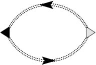
Figure 2: Dynamical susceptibility. Triangles refer to external measurement vertices. The black (emission) vertex is renormalized like the interaction vertex in Fig. 1, except that the two external $ce$ legs are removed. The other (absorption) vertex remains undressed.

II.3 Dynamical spin susceptibility

In order to uncover the physical meaning of the rate $\Gamma_{\!s}$ introduced in Eq. (II.2.3), we include here a brief discussion of the transverse spin susceptibility:

$${{}^{\perp}}\chi^{R}(t)=i\theta(t)\langle[S^{-}(t),S^{+}(0)]\rangle.$$ (59)

The transverse spin relaxation rate, $\Gamma_{2}$, is defined as the broadening of the resonance pole in this response function, and as will be shown below, $\Gamma_{\!s}$ plays exactly this role. Throughout this Section, we may therefore use $\Gamma_{\!s}=\Gamma_{2}$. With a suitable generalization of $\Gamma_{v}$, entering Eq. (II.2.3), which will be given in Sec. IV, this identification holds also for anisotropic coupling.

Translating to the pseudo fermion representation on the Keldysh contour, the transverse susceptibility is calculated from

$${{}^{\perp}}\chi(\tau)=-i(-i)^{2}\langle T_{c_{K}}\{f^{\dagger}_{\downarrow}(\tau)f_{\uparrow}(\tau)f^{\dagger}_{\uparrow}(0)f_{\downarrow}(0)\}\rangle,$$ (60)

which in turn leads to the Feynman diagram in Fig. 2 when including vertex, and $pf$ self-energy corrections. The bare absorption, and emission vertices are given as $\gamma^{1}_{ab}=\frac{1}{\sqrt{2}}\delta_{ab}$ and ${\tilde{\gamma}}^{1}_{ab}=\frac{1}{\sqrt{2}}\tau^{1}_{ab}$, respectively (cf. I). The absorption vertex is kept undressed and the emission vertex renormalizes like the interaction vertex-component $\sqrt{2}{\tilde{\Lambda}}{{}_{ab}}\!\!\!\!\!{{}^{11}}$, whereby

$${{}^{\perp}}\chi^{R}(\Omega)=i\int\frac{d\omega}{2\pi}{\tilde{\Lambda}}{{}_{ab}}\!\!\!\!\!{{}^{11}}(\Omega+\omega,\omega)\underline{\cal G}_{\uparrow}^{bc}(\Omega+\omega)\underline{\cal G}_{\downarrow}^{ca}(\omega).$$ (61)

Notice that the canonical ensemble average, enforcing single occupancy on the dot, is carried out by dividing the $\lambda$-dependent grand-canonical average by $\langle Q\rangle_{\lambda}$ and taking the limit $\lambda\to\infty$ (cf. I). This procedure affects only the $pf$ distribution functions and allows to neglect all terms proportional to squares, or higher powers of $n_{\gamma\lambda}$. Working out the contractions, we arrive at

$${{}^{\perp}}\chi^{R}(\Omega) = i\int\frac{d\omega}{2\pi}\Bigl{\{}\,\,\!\!\ ^{0\!}{\tilde{\Lambda}}{{}_{21}}\!\!\!\!\!{{}^{11}}(\Omega+\omega,\omega)2\left[n_{\downarrow}(\omega)-n_{\uparrow}(\Omega+\omega)\right]{\cal G}^{R}_{\uparrow}(\Omega+\omega){\cal G}^{A}_{\downarrow}(\omega)$$ (62)

$$\hskip 34.1433pt+\left[{{}^{\lambda\!}}{\tilde{\Lambda}}{{}_{11}}\!\!\!\!\!{{}^{11}}(\Omega+\omega,\omega)+{{}^{\lambda\!}}{\tilde{\Lambda}}{{}_{21}}\!\!\!\!\!{{}^{11}}(\Omega+\omega,\omega)-2n_{\downarrow}(\omega){{}^{0\!}}{\tilde{\Lambda}}{{}_{21}}\!\!\!\!\!{{}^{11}}(\Omega+\omega,\omega)\right]{\cal G}^{R}_{\uparrow}(\Omega+\omega){\cal G}^{R}_{\downarrow}(\omega)$$

$$\hskip 34.1433pt+\left[{{}^{\lambda\!}}{\tilde{\Lambda}}{{}_{22}}\!\!\!\!\!{{}^{11}}(\Omega+\omega,\omega)-{{}^{\lambda\!}}{\tilde{\Lambda}}{{}_{21}}\!\!\!\!\!{{}^{11}}(\Omega+\omega,\omega)+2n_{\uparrow}(\Omega+\omega){{}^{0\!}}{\tilde{\Lambda}}{{}_{21}}\!\!\!\!\!{{}^{11}}(\Omega+\omega,\omega)\right]{\cal G}^{A}_{\uparrow}(\Omega+\omega){\cal G}^{A}_{\downarrow}(\omega)\Bigr{\}}.$$

The important fact that the final result is proportional to $n_{\gamma}$ is ensured by the relations

$${{}^{0\!}}{\tilde{\Lambda}}{{}_{21}}\!\!\!\!\!{{}^{11}}+{{}^{0\!}}{\tilde{\Lambda}}{{}_{11}}\!\!\!\!\!{{}^{11}}={{}^{0\!}}{\tilde{\Lambda}}{{}_{21}}\!\!\!\!\!{{}^{11}}-{{}^{0\!}}{\tilde{\Lambda}}{{}_{22}}\!\!\!\!\!{{}^{11}}=1,$$ (63)

as such a constant drops after integrating over ${\cal G}^{R}{\cal G}^{R}$ or ${\cal G}^{A}{\cal G}^{A}$.

In the limit of $B\to 0$, the factor of $n_{\downarrow}(\omega)-n_{\uparrow}(\Omega+\omega)$ in the first term is of order $\Omega/V$, and therefore we are forced to keep also the other terms involving ${\cal G}^{R}{\cal G}^{R}$ or ${\cal G}^{A}{\cal G}^{A}$. In this case, we have to keep the full dependence of the vertex on two frequencies, but since for example the parts of the vertex which are retarded with respect to $\omega$ integrate to zero with ${\cal G}^{R}{\cal G}^{R}$, matters simplify substantially. The first square bracket can simply be replaced by

$$\left[\frac{2n_{\lambda}(0)\Pi^{<}(\omega)-2\Pi^{>}(\omega)n_{\lambda}(\omega)}{\Omega+i\Gamma_{2}}-in_{\lambda}(\omega)\right],$$ (64)

and inserting now the nonequilibrium distribution function given by (38), the first two terms of this expression are seen to cancel. We emphasize the fact that this important cancellation takes place only when using the correct distribution function, i.e. the solution to the quantum Boltzmann equation corresponding to second order $pf$ self-energies.

The term involving ${\cal G}^{A}{\cal G}^{A}$ works in a similar way, and using the approximation ${\cal G}^{R/A}_{\uparrow}(\Omega+\omega){\cal G}^{R/A}_{\downarrow}(\omega)\approx-\partial_{\omega}(\omega\pm i0_{+})^{-1}$, valid to leading order in $\max(|\Omega|,\Gamma)/V$ when integrated with the slowly varying distribution function, the last two terms in (62) may be evaluated by partial integration. The first term comes with a factor of ${{}^{0\!}}{\tilde{\Lambda}}{{}_{21}}\!\!\!\!\!{{}^{11}}(\Omega+\omega,\omega){\cal G}^{R}_{\uparrow}(\Omega+\omega){\cal G}^{A}_{\downarrow}(\omega)\approx 2\pi i\delta(\omega)/(\Omega+i\Gamma_{2})$, and altogether one finds that

$${{}^{\perp}}\chi^{R}(\Omega)\approx\frac{M}{B}\frac{i\Gamma_{2}}{\Omega+i\Gamma_{2}},$$ (65)

for $\max(|\Omega|,\Gamma)\ll V$. The prefactor is independent of $B$ and is obtained as the derivative $-n^{\prime}(0)$, with $n(\omega)$ given by (39) and with the replacement $n_{\lambda}(0)\to 1/2$, due to the normalization by $\langle Q\rangle_{\lambda}$ before projection. The zero-frequency limit obeys ${{}^{\perp}}\chi^{R}(0)=M/B$, like in equilibrium, and the nonequilibrium magnetization was found in I to be

$$M=\frac{(g_{LL}^{2}+g_{RR}^{2}+2g_{LR}^{2})B}{2g_{LR}^{2}V},$$ (66)

similar to a Curie-law with $1/T$ replaced by $4/V$. Notice that the result (65), has been obtained also in Ref. Mao03, , using a Majorana-fermion representation.

In the case of a finite magnetic field, the factor of $n_{\downarrow}(\omega)-n_{\uparrow}(\Omega+\omega)$ in the first term of (62) will be of order $B/V$. For $B\gg\max(|\Omega+B|,\Gamma)$, this term will therefore dominate the other terms involving ${\cal G}^{R}{\cal G}^{R}$ or ${\cal G}^{A}{\cal G}^{A}$. For $B>0$, the vertex renormalization is modified, but since we only need to consider the first term in (62), only a single component is needed. For this particular component the generalization is straightforward and one finds that

$${{}^{0\!}}{\tilde{\Lambda}}{{}_{21}}\!\!\!\!\!{{}^{11}}(\Omega+\omega,\omega)=\frac{1}{2}\left(1-\frac{2i\Pi^{>}(\omega-B/2)}{\Omega+B+i\Gamma_{2}}\right),$$ (67)

where $\Gamma_{2}$ is given in Eq. (II.2.3) and depends now on both $V$ and $B$ (see Eq. (70) below). The integral over $\omega$ is performed using the approximation (37), and the susceptibility is found to be

$${{}^{\perp}}\chi^{R}(\Omega)\approx\frac{M}{\Omega+B+i\Gamma_{2}},$$ (68)

valid for $\max(|\Omega+B|,\Gamma)\ll\min(B,V)$

In the intermediate regime where $B\ll\min(|\Omega+B|,\Gamma)$, one would need to generalize also the $\lambda$-dependent part of the vertex to the case of $B>0$. However, we expect that cancellations, similar to those found in terms like (64) at zero field, will take place also at finite $B$, once the correct $B$-dependent distribution function is used. In this manner, we expect the general formula for the susceptibility to be simply

$${{}^{\perp}}\chi^{R}(\Omega)\approx\frac{M}{B}\frac{B+i\Gamma_{2}}{\Omega+B+i\Gamma_{2}},$$ (69)

valid for $\max(|\Omega+B|,\Gamma)\ll V$. This function obviously has the correct asymptotic behaviors, corresponding to (65) and (68), and is consistent with the equilibrium resultWalker68 ; Woelfle71 .

For completeness, we state here the relevant asymptotics of $\Gamma_{2}$ as a function of $V$, $B$ and $T$:

$$\Gamma_{2}\approx\left\{\begin{array}[]{ll}\pi g_{LR}^{2}V&,\,\max(T,B)\ll V\\ &\\ \pi(g_{LL}^{2}+g_{RR}^{2})B/4&,\,\max(T,V)\ll B\\ &\\ \pi(g_{LL}^{2}+g_{RR}^{2}+2g_{LR}^{2})T&,\,\max(B,V)\ll T\end{array}\right.$$ (70)

In the equilibrium limit, $V=0$, this corresponds to the result obtained in Refs. Walker68, and Woelfle71, , $\Gamma_{2}\approx\pi g^{2}\max(T,B/4)$.

III Conduction electron T-matrix

With the renormalized vertex at hand, we now proceed to calculate the conduction electron T-matrix, including the leading logarithmic corrections. The T-matrix, $T_{\alpha\alpha^{\prime}}$, is of great physical significance, insofar as it describes the scattering of conduction electrons from lead $\alpha^{\prime}$ to lead $\alpha$, and thereby also the transport across the dot. It is determined from the conduction electron Green function:

$$G^{R}_{\alpha\alpha^{\prime},\sigma}(\omega)=G^{R(0)}_{\alpha\sigma}(\omega)\delta_{\alpha\alpha^{\prime}}+G^{R(0)}_{\alpha\sigma}(\omega){\rm T}^{R}_{\alpha\alpha^{\prime},\sigma}(\omega)G^{R(0)}_{\alpha^{\prime}\sigma}(\omega).$$ (71)

In cases where the exchange-tunneling Hamiltonian (2) is derived from an underlying Anderson model, i.e. from a single quantum dot in the Coulomb-blockade regime (cf. e.g. Ref. Kaminski99, ), one has $J_{LR}^{2}=J_{LL}J_{RR}$ and only one of the eigenvalues of the $2\times 2$ matrix $T_{\alpha\alpha^{\prime}}$ is finite. In such a

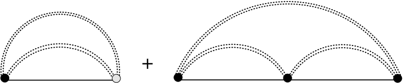
Figure 3: Diagrams for the conduction electron T-matrix, with dressed $pf$ propagators and dressed interaction vertices (black dots).

situation, $\text{Im}[{\rm T}_{\alpha\alpha^{\prime}\sigma}(\omega)]$ is, at low energies, directly proportional to the spectral function of the electrons on the dot (see e.g. Ref. Rosch03b, and references therein). This spectral function can be measured directly by tunneling into the dotFranceschi02 , and henceforth we shall focus on the imaginary part of $T_{\alpha\alpha^{\prime}}$.

In Fig. 3 we show the two diagrams contributing to the T-matrix to third order. Within bare perturbation theory (i.e. using bare vertices and Green functions in Fig. 3), one obtains the following intra- and inter-lead components at $T,B=0$:

$$\text{Im}\left[{\rm T}_{\alpha\alpha}^{R}(\Omega)\right] = -\frac{3\pi}{16N(0)}\left\{(g_{\alpha\alpha}^{2}+g_{LR}^{2})\left[1+2g_{\alpha\alpha}\ln\left(\frac{D}{|\Omega-\mu_{\alpha}|}\right)\right]+4g_{d}g_{LR}^{2}\ln\left(\frac{D}{|\Omega+\mu_{\alpha}|}\right)\right\},$$ (72)

$$\text{Im}\left[{\rm T}_{LR}^{R}(\Omega)\right] = -\frac{3\pi}{16N(0)}g_{LR}\left\{2g_{d}\left[1+2g_{LL}\ln\left(\frac{D}{|\Omega-\mu_{\alpha}|}\right)\right]+2(g_{RR}^{2}+g_{LR}^{2})\ln\left(\frac{D}{|\Omega-\mu_{R}|}\right)\right\},$$ (73)

with $\mu_{L}=-\mu_{R}=V/2$. Within bare perturbation theory, the T-matrix diverges close to each Fermi surface, or more precisely, for $\Omega\to\mu_{\alpha}$, some of the logarithms are cut off by the voltage $V=\mu_{L}-\mu_{R}$ while others remains unaffected. In this sense voltage and temperature act very differently as $T$ would cut off all logarithmic terms uniformly. The central question formulated in the introduction is, how the logarithmic divergences which remain for $T\to 0$ and large $V$ are cut off when the perturbation theory is properly resummed. To find the correct cut-off to order $g^{2}$, we have to replace the bare Green functions and bare vertices in Fig. 3 by the dressed ones.

As the second-order diagram in Fig. 3 gives only a finite contribution $\text{Im}[{\rm T}_{\alpha\alpha^{\prime}}^{R}(\Omega)]=-\frac{3\pi}{16N(0)}\sum_{\alpha^{\prime\prime}}g_{\alpha\alpha^{\prime\prime}}g_{\alpha^{\prime\prime}\alpha^{\prime}}$, the inclusion of self-energy, and vertex corrections will produce only subleading corrections of order $g^{4}$, as can be shown by an explicit calculation.

The fate of the logarithms arising to order $g^{3}$ is more interesting, and in the following we will therefore carefully evaluate the second diagram in Fig. 3. This contribution involves the spin-contractions

$$\tau^{k}_{\gamma\gamma^{\prime}}\tau^{j}_{\gamma^{\prime}\gamma^{\prime\prime}}\tau^{i}_{\gamma^{\prime\prime}\gamma}\tau^{i}_{\sigma\sigma^{\prime\prime}}\tau^{j}_{\sigma^{\prime\prime}\sigma^{\prime}}\tau^{k}_{\sigma^{\prime}\sigma}=24$$ (74)

for the Peierls, and

$$\tau^{i}_{\gamma\gamma^{\prime\prime}}\tau^{j}_{\gamma^{\prime\prime}\gamma^{\prime}}\tau^{k}_{\gamma^{\prime}\gamma}\tau^{i}_{\sigma\sigma^{\prime\prime}}\tau^{j}_{\sigma^{\prime\prime}\sigma^{\prime}}\tau^{k}_{\sigma^{\prime}\sigma}=-24$$ (75)

for the Cooper-channel. Writing out the sum of these two types of diagrams, corresponding to different orientations of the $pf$-loop, one finds that

$${\rm T}_{\alpha\alpha^{\prime}}^{R(3)}(\Omega) = \frac{24}{2}(-1)^{1}(i)^{3}(J_{\alpha\alpha^{\prime\prime}}J_{\alpha^{\prime\prime}\alpha^{\prime\prime\prime}}J_{\alpha^{\prime\prime\prime}\alpha^{\prime}}/4^{3})\!\int\!\frac{d\omega}{2\pi}\!\int\!\frac{d\varepsilon}{2\pi}\!\int\!\frac{d\varepsilon^{\prime}}{2\pi}{\underline{G}}_{\alpha^{\prime\prime}}^{d^{\prime\prime}\!c^{\prime\prime}}(\Omega+\varepsilon){\underline{G}}_{\alpha^{\prime\prime\prime}}^{d^{\prime}\!c^{\prime}}(\Omega+\varepsilon^{\prime})$$ (76)

$$\hskip 8.53581pt\times\left\{{\tilde{\Lambda}}^{1d^{\prime\prime}}_{a^{\prime\prime}\!b}(\omega,\omega+\varepsilon){\underline{\cal G}}^{ba}(\omega){\tilde{\Lambda}}^{c^{\prime}\!1}_{ab^{\prime}}(\omega+\varepsilon^{\prime},\omega){\underline{\cal G}}^{b^{\prime}\!a^{\prime}}(\omega+\varepsilon^{\prime}){\tilde{\Lambda}}^{c^{\prime\prime}\!d^{\prime}}_{a^{\prime}\!b^{\prime\prime}}(\omega+\varepsilon,\omega+\varepsilon^{\prime}){\underline{\cal G}}^{b^{\prime\prime}\!a^{\prime\prime}}(\omega+\varepsilon)\right.$$

$$\left.\hskip 15.649pt-{\tilde{\Lambda}}^{c^{\prime}\!1}_{a^{\prime}\!b}(\omega,\omega-\varepsilon^{\prime}){\underline{\cal G}}^{ba}(\omega){\tilde{\Lambda}}^{1d^{\prime\prime}}_{ab^{\prime\prime}}(\omega-\varepsilon,\omega){\underline{\cal G}}^{b^{\prime\prime}\!a^{\prime\prime}}(\omega-\varepsilon){\tilde{\Lambda}}^{c^{\prime\prime}\!d^{\prime}}_{a^{\prime\prime}\!b^{\prime}}(\omega-\varepsilon^{\prime},\omega-\varepsilon){\underline{\cal G}}^{b^{\prime}\!a^{\prime}}(\omega-\varepsilon^{\prime})\right\}.$$

This Keldysh contraction has a total of 256 terms, of which only a few will contribute in the end. Some will involve a ${\underline{\cal G}}^{21}$, which is zero, and others will involve a product of more than one lesser-component ${\cal G}^{<}$, which, being proportional to higher powers of the $pf$ distribution function, will vanish faster than $\langle Q\rangle_{\lambda}$. Since the Keldysh representation contains ${\cal G}^{<}$ as part of ${\cal G}^{K}={\cal G}^{<}+{\cal G}^{>}$, it is a daunting task to isolate all contractions with only one factor of ${\cal G}^{<}$. Nevertheless, since we are dealing here with a trace over the $pf$ Keldysh indices, we are free to work in a more convenient basis for the pseudo fermions. Thus choosing

$$\zeta=\left(\begin{array}[]{rr}1&1\\ 0&1\end{array}\right),\hskip 14.22636pt\zeta^{-1}=\left(\begin{array}[]{rr}1&-1\\ 0&1\end{array}\right),$$ (77)

the Keldysh matrix Green functions may be transformed as

$${\hat{\cal G}}=\zeta\,{\underline{\cal G}}\,\zeta^{-1}=\left(\begin{array}[]{cc}{\cal G}^{R}&2{\cal G}^{<}\\ 0&{\cal G}^{A}\end{array}\right),$$ (78)

which has the nice property that ${\hat{\cal G}}$ becomes diagonal after projection. The renormalized vertices may be considered as functions of only one frequency and therefore take the form (56), which we write loosely as $\Lambda=\delta+L$. For opposite $ce$ Keldysh-indices the vertex retains the structure of the identity-matrix $\delta$ under the transformation. For equal $ce$-indices, the matrix $L_{ab}$ transforms to

$${\hat{L}}=\zeta L\,\zeta^{-1}={{}^{0\!}}{\hat{L}}+{{}^{\lambda\!}}{\hat{L}},$$ (79)

where

$${}^{0\!}{\hat{L}}=\left(\begin{array}[]{cc}1&0\\ \phi&-1\end{array}\right),$$ (80)

and

$${}^{\lambda\!}{\hat{L}}=2n_{\lambda}(0)\left(\begin{array}[]{cc}\frac{\psi^{\ast}}{2}-\frac{4\Gamma_{\!s}\Pi^{R}(0)}{\Omega^{2}+\Gamma_{\!s}^{2}}&\psi\\ 0&-\frac{\psi^{\ast}}{2}-\frac{4\Gamma_{\!s}\Pi^{A}(0)}{\Omega^{2}+\Gamma_{\!s}^{2}}\end{array}\right),$$ (81)

with $\phi=\frac{\Omega+i\Gamma}{\Omega+i\Gamma_{\!s}}$ and $\psi=\frac{2i\Gamma_{v}}{\Omega-i\Gamma_{\!s}}$.

In this representation the contraction in Eq. (76) becomes manageable and one has to deal with merely 8 different types of terms. The full contraction is worked out in Appendix B, resulting in

$${\rm T}_{\alpha\alpha^{\prime}}^{R(3)}(\Omega)=\frac{3}{16}n_{\lambda}J^{3}_{\alpha\alpha^{\prime\prime}\alpha^{\prime\prime\prime}\alpha^{\prime}}\!\int\!\frac{d\varepsilon}{2\pi}\!\int\!\frac{d\varepsilon^{\prime}}{2\pi}$$

$$\times\left\{G_{\alpha^{\prime\prime}}^{K}(\Omega+\varepsilon)G_{\alpha^{\prime\prime\prime}}^{R}(\Omega+\varepsilon^{\prime}){\cal G}^{A}_{\Gamma_{\!s}}(\varepsilon){\cal G}^{A}_{\Gamma_{\!s}}(\varepsilon^{\prime})\right.$$

$$\hskip 11.38109pt-\left[G_{\alpha^{\prime\prime}}^{R}(\Omega+\varepsilon)G_{\alpha^{\prime\prime\prime}}^{K}(\Omega+\varepsilon^{\prime})\right.$$

$$\left.\left.\hskip 21.33955pt+G_{\alpha^{\prime\prime}}^{K}(\Omega+\varepsilon)G_{\alpha^{\prime\prime\prime}}^{A}(\Omega+\varepsilon^{\prime})\right]{\cal G}^{A}_{\Gamma_{\!s}}(\varepsilon){\cal G}^{A}_{\Gamma_{\!s}}(\varepsilon-\varepsilon^{\prime})\right\},$$

where ${\cal G}^{A}_{\Gamma_{\!s}}(\varepsilon)=1/(\varepsilon-i\Gamma_{\!s})$ are Green functions broadened by $\Gamma_{\!s}$ rather than $\Gamma/2$ and we use the shorthand notation $J^{3}_{\alpha\alpha^{\prime\prime}\alpha^{\prime\prime\prime}\alpha^{\prime}}=J_{\alpha\alpha^{\prime\prime}}J_{\alpha^{\prime\prime}\alpha^{\prime\prime\prime}}J_{\alpha^{\prime\prime\prime}\alpha^{\prime}}$. Already at this stage, it is apparent that the vertex corrections have served to replace twice the $pf$ self-energy broadening by $\Gamma_{\!s}$. Making use of the basic integrals,

$$\int_{-D}^{D}\!d\varepsilon\,\frac{{\rm sgn}(\varepsilon+a)(\varepsilon+b)}{(\varepsilon+b)^{2}+\Gamma_{\!s}^{2}}=\ln\left(\frac{D^{2}}{(b-a)^{2}+\Gamma_{\!s}^{2}}\right)$$ (83)

and

$$\int_{-D}^{D}\!d\varepsilon\,\frac{{\rm sgn}(\varepsilon+a)\Gamma}{(\varepsilon+b)^{2}+\Gamma_{\!s}^{2}}=2\tan^{-1}\left(\frac{b-a}{\Gamma_{\!s}}\right),$$ (84)

representing a broadened logarithm and a broadened sign-function, respectively, the remaining integrals over $\varepsilon$ and $\varepsilon^{\prime}$ are straightforward.

The first line of the integral (III) involves a convolution of $G^{K}$ with ${\cal G}^{A}$, which yields

$$-iN(0)\left\{\ln\left(\frac{D^{2}}{(\Omega-\mu_{\alpha^{\prime\prime}})^{2}+\Gamma_{\!s}^{2}}\right)+2i\tan^{-1}\left(\frac{\Omega-\mu_{\alpha^{\prime\prime}}}{D}\right)\right\}.$$

This term is multiplied by the convolution of $G_{\alpha^{\prime}}^{R}$ with ${\cal G}^{A}_{\Gamma}$, equal to $iG_{\alpha^{\prime}}^{R}(\Omega+i\Gamma)$, and altogether the first line yields the imaginary part

$$-2n_{\lambda}\frac{3\pi}{32}J^{3}_{\alpha\alpha^{\prime\prime}\alpha^{\prime\prime\prime}\alpha^{\prime}}N(0)^{2}\ln\left(\frac{D^{2}}{(\Omega-\mu_{\alpha^{\prime\prime}})^{2}+\Gamma_{\!s}^{2}}\right).$$ (85)

Using a spectral representation for the $ce$ Green functions, the remaining two lines of (III) can be brought to the form

$$2n_{\lambda}\frac{3}{32}J^{3}_{\alpha\alpha^{\prime\prime}\alpha^{\prime\prime\prime}\alpha^{\prime}}N(0)^{2}\!\int_{-D}^{D}\!\frac{d\varepsilon}{2\pi}\,\!\int_{-D}^{D}\!d\omega\,$$ (86)

$$\hskip 45.5244pt\times\!\left[\,\frac{{\rm sgn}(\varepsilon-\mu_{\alpha^{\prime\prime\prime}})}{(\omega-\Omega-i\Gamma_{\!s})(\omega-\varepsilon-i\Gamma_{\!s})}\right.$$

$$\hskip 51.21495pt\left.+\frac{{\rm sgn}(\varepsilon-\mu_{\alpha^{\prime\prime}})}{(\varepsilon-\Omega-i\Gamma_{\!s})(\omega-\varepsilon+i\Gamma_{\!s})}\,\right].$$

The $\omega$ integral in first term vanishes in the limit $D\to\infty$, and keeping $D$ finite this term remains smaller than the second term by a factor of $\Omega/D$ or $\Gamma_{\!s}/D$. Keeping only the second term, the imaginary part takes exactly the same form as (85), and finally we obtain after projection

$$\text{Im}\left[{\rm T}_{\alpha\alpha}^{R}(\Omega)\right]=-\frac{3\pi}{16N(0)}\left\{(g_{\alpha\alpha}^{2}+g_{LR}^{2})\left[1+g_{\alpha\alpha}\ln\left(\frac{D^{2}}{(\Omega-\mu_{\alpha})^{2}+\Gamma_{\!s}^{2}}\right)\right]+2g_{LR}^{2}g_{d}\ln\left(\frac{D^{2}}{(\Omega+\mu_{\alpha})^{2}+\Gamma_{\!s}^{2}}\right)\right\},$$ (87)

with no summation over $\alpha$ implied. We find precisely the result of bare perturbation theory, Eq. (72), but now with the logarithmic divergences cut off by $\Gamma_{\!s}$. The same conclusion also holds for ${\rm T}_{LR}$. This is the central result of this paper.

IV Anisotropic Couplings: $T_{1}$ vs. $T_{2}$

The longitudinal, and the transverse spin-relaxation rates, $1/T_{1}$ and $1/T_{2}$, have rather different physical interpretations. It is therefore interesting to determine which combination of the two rates actually controls the logarithmic divergences. In the previous chapter we restricted ourselves to the case of zero magnetic field and isotropic couplings, and in this case we cannot distinguish between the two rates as $1/T_{1}=1/T_{2}=\Gamma_{\!s}$.

To discriminate between the two rates, even for $B=0$, we generalize the exchange interaction to involve two different couplings

$${{}^{\bot\!\!}}J_{\alpha^{\prime}\alpha}(\tau^{1}_{\gamma^{\prime}\gamma}\tau^{1}_{\sigma^{\prime}\sigma}+\tau^{2}_{\gamma^{\prime}\gamma}\tau^{2}_{\sigma^{\prime}\sigma})+{{}^{z\!\!}}J_{\alpha^{\prime}\alpha}\tau^{3}_{\gamma^{\prime}\gamma}\tau^{3}_{\sigma^{\prime}\sigma},$$ (88)

and we may now repeat all calculations above, keeping track of separate spin-flip and non-spin-flip processes. Since we consider only the case of zero magnetic field, the $pf$ self-energy broadening remains spin-independent and we obtain from Eq. (29), for $V\gg T$ and $B=0$,

$$\Gamma=\Gamma_{\uparrow}=\Gamma_{\downarrow}=\frac{\pi}{4}({{}^{z\!}}g_{LR}^{2}+2\,{{}^{\bot\!}}g_{LR}^{2})V.$$ (89)

The vertex corrections now take a different form, depending on whether or not the spin is flipped at the vertex. For $T=B=0$ and finite $V$ we obtain $\Gamma_{v}^{\perp}=\pi\,{{}^{z\!}}g_{LR}^{2}V/4$ for the spin-flip vertex and $\Gamma_{v}^{z}=\pi(2\,{{}^{\bot\!}}g_{LR}^{2}-\,{{}^{z\!}}g_{LR}^{2})V/4$ in the case of no spin-flip. Therefore, the longitudinal, and the transverse spin-relaxation rates are given by

$$\frac{1}{T_{1}}=\Gamma_{1}=\Gamma+\Gamma_{v}^{z}=\pi\,{{}^{\bot\!}}g_{LR}^{2}V,$$ (90)

and

$$\frac{1}{T_{2}}=\Gamma_{2}=\Gamma+\Gamma_{v}^{\perp}=\frac{\pi}{2}({{}^{z\!}}g_{LR}^{2}+{{}^{\bot\!}}g_{LR}^{2})V.$$ (91)

Notice that $1/T_{1}=0$ for ${}^{\perp}\!g=0$. This is due to a cancellation of vertex, and self-energy corrections, reflecting the conservation of $S_{z}$ in this case.

How do these spin-relaxation rates modify the logarithmic divergences? A close inspection of the Keldysh contractions and the integrals carried out in Appendix B reveals that only the ${{}^{0\!}}\Lambda$-part of the renormalized vertex connecting to the out-going $ce$-line (i.e. the left most vertex in Fig. 3) gives rise to a logarithmic divergence, and furthermore determines whether this logarithm is cut off by $\Gamma_{2}$ or $\Gamma_{1}$ depending on whether this vertex involves a spin-flip or not. Therefore, in the case of anisotropic couplings, Eq. (87) generalizes to

$$\text{Im}\left[{\rm T}_{\alpha\alpha^{\prime}}^{R}(\Omega)\right] = -\frac{\pi}{16N(0)}\sum_{\alpha^{\prime\prime},\alpha^{\prime\prime\prime}}\left\{\,\,\,{{}^{z\!}}g_{\alpha\alpha^{\prime\prime}}\left[{{}^{z\!}}g_{\alpha^{\prime\prime}\alpha^{\prime}}+{{}^{\bot\!}}g_{\alpha^{\prime\prime}\alpha^{\prime\prime\prime}}{{}^{\bot\!}}g_{\alpha^{\prime\prime\prime}\alpha^{\prime}}\ln\left(\frac{D^{2}}{(\Omega-\mu_{\alpha^{\prime\prime}})^{2}+\Gamma_{1}^{2}}\right)\right]\right.$$

$$\hskip 71.55865pt\left.+{{}^{\bot\!}}g_{\alpha\alpha^{\prime\prime}}\left[2\,{{}^{\bot\!}}g_{\alpha^{\prime\prime}\alpha^{\prime}}+\left({{}^{z\!}}g_{\alpha^{\prime\prime}\alpha^{\prime\prime\prime}}{{}^{\bot\!}}g_{\alpha^{\prime\prime\prime}\alpha^{\prime}}+{{}^{\bot\!}}g_{\alpha^{\prime\prime}\alpha^{\prime\prime\prime}}{{}^{z\!}}g_{\alpha^{\prime\prime\prime}\alpha^{\prime}}\right)\ln\left(\frac{D^{2}}{(\Omega-\mu_{\alpha^{\prime\prime}})^{2}+\Gamma_{2}^{2}}\right)\right]\right\}.$$

Roughly speaking, two thirds of the logarithms are broadened by $\Gamma_{2}$ and one third by $\Gamma_{1}$.

How are these results modified beyond lowest order perturbation theory? In Appendix C we investigate this question in the limit ${}^{\perp}\!g\to 0$ for finite ${}^{z}\!g$. In this limit, the logarithmic singularities in correlation functions like $\langle S^{-}S^{+}\rangle$ resum in equilibrium to power-laws with exponents depending on ${}^{z}\!g$. In Appendix C we use a mapping of our problem to a non-equilibrium X-ray edge problem together with results by NgNg96 and othersCombescot00 ; Muzykantskii03 to investigate how these power-law singularities are affected by a finite bias voltage and the associated current. We find that all these power-laws are cut off by a rate related to $1/T_{2}$. This has a simple interpretation: for finite ${}^{z}\!\!J$ a finite current is flowing through the system and the corresponding noise prohibits the coherence of the two external spin-flips at low energy. Close inspection reveals, that the second logarithm in Eq. (IV) is calculated from a correlation function of the type discussed in Appendix C. The non-perturbative results of the Appendix therefore confirm our perturbative Eq. (IV). The first logarithm in Eq. (IV), however, arises from a different correlator (as one external vertex involves $S_{z}$) which we have not tried to calculate to higher orders in ${}^{z}\!g$.

Also in the presence of a magnetic field the situation is more complex and at present we do not know which combination of relaxation rates controls the logarithmic divergences arising for $V\approx B$. The vertex corrections depend on $B$ and, as mentioned in Sec. II.2.3, also the $\tau^{1}_{cd}$-part of the vertex renormalizes in this case. Furthermore, the non-spin-flip vertex depends on the orientation of the incoming spin, and its two different components are found only after solving two coupled vertex equations (cf. e.g. Ref. Walker68, ).

In many physical situations, $1/T_{1}$ and $1/T_{2}$ differ only by a numerical prefactor of order $1$ and such a factor in the argument of the logarithms is not important. In this situations it is not necessary to keep track of differences of $1/T_{1}$ and $1/T_{2}$, if one is interested in a calculation to leading order in $1/\ln[\max(V,B)/T_{K}]$ (cf. e.g. Ref. Rosch03a, ).

V Discussion

In this paper we have addressed the question how, far out of equilibrium, the presence of a sufficiently large current prohibits the coherent spin-flips necessary for the development of the Kondo effect. In an explicit calculation, we have confirmed the expected answer Wolf69 ; Meir93 ; Kaminski99 ; Rosch01 ; Rosch03a that the spin-relaxation rate cuts off the logarithmic corrections of perturbation theory. This implies that for $\Gamma_{\!s}\gg T_{K}$ (i.e. for $V\gg T_{K}$, see Refs. Rosch01, ; Rosch03a, ), the Kondo-model stays in the perturbative regime, which allows calculating its properties in a controlled way using perturbative renormalization group Rosch03a .

We have worked out this scenario explicitly for the imaginary part of the conduction electron T-matrix, taking into account the joint effect of self-energy, and vertex corrections. In the limit of zero temperature and $\ln(V/T_{K})\gg 1$, perturbation theory remains valid and the vertex corrections were determined by summing up diagrams to leading order in $\Gamma/V\sim g^{2}$. Within bare perturbation theory, the T-matrix exhibits logarithmic divergences at the Fermi energies of the left, and the right lead, and we have demonstrated explicitly that the joint effect of dressing $pf$ Green functions as well as exchange vertices with voltage induced particle-hole excitations works to cut off these logarithms by $\Gamma_{\!s}=\pi g_{LR}^{2}V$. Under certain conditions, the T-matrix can be identified with the spectral function on the quantum dot, which can be measured directly by tunneling into the dotFranceschi02 .

To reveal the physical significance of this rate, we have calculated the dynamical transverse spin susceptibility in the presence of a finite bias-voltage. This served to demonstrate that $\Gamma_{\!s}$ is indeed the spin-relaxation rate, broadening the resonance pole at $\omega\sim B$ in this correlation function. $\Gamma_{\!s}$ arises from the stirring up of inter-lead particle-hole excitations, and is found to be proportional, in order $g^{2}$, to the number of conduction electrons passing the constriction per unit time (the factor of proportionality depends, however, on details of the model, such as e.g. anisotropies of $J$). We therefore interpret the subsequent attenuation of the Kondo effect as decoherence due to current-induced noise.

Most formulations of perturbative renormalization group in equilibrium completely neglect the role of decoherence and noise and focus instead on the flow of coupling constants. This is justified, as the typical rates are often much smaller than temperature $T$, which serves as the relevant infrared cutoff. However, since this is not the case in a nonequilibrium situation, decoherence has to be an essential ingredient in any formulation of perturbative renormalization group valid out of equilibriumSchoeller00 ; Rosch03a . We hope that our perturbative calculation, demonstrating how this happens in detail, can serve as a starting point for future developments in this direction.

Appendix A Vertex corrections from crossed rungs

In this Appendix, we argue that crossed diagrams of the form shown in Fig. 4 lead only to subleading corrections. In such diagrams, for example, the simple frequency dependence observed in Sec. II.2.3 is no longer valid. We therefore evaluate explicitly the crossed 4th order correction depicted in Fig.4 and compare it to (50).

The Feynman rules give the same prefactors in this case, and the contraction of spins yields

$$(\tau^{i}\tau^{j}\tau^{k}\tau^{m}\tau^{n})_{\gamma^{\prime}\gamma}{\rm Tr}[\tau^{m}\tau^{j}]{\rm Tr}[\tau^{i}\tau^{n}]=20\,\tau^{k}_{\gamma^{\prime}\gamma},$$ (93)

as opposed to $4\,\tau^{k}_{\gamma^{\prime}\gamma}$ obtained in the ladder-type correction. The Keldysh contraction may be expressed in terms of the previously defined tensors $V$ and $B$ as

$$V{{}_{\!a^{\prime}\!b^{\prime}}}\!\!\!\!\!{{}^{\!\!c\,d}}\,(\Omega+\omega,\omega)B{{}_{b^{\prime\prime}\!a}}\!\!\!\!\!{{}^{\!\!a^{\prime}b^{\prime\prime\prime}}}\!(\omega^{\prime}-\omega){\underline{\cal G}}^{b^{\prime\prime\prime}a^{\prime\prime}}\!(\Omega+\omega^{\prime})$$ (94)

$$\times\,{\underline{\cal G}}^{b^{\prime\prime}a^{\prime\prime\prime}}\!(\omega+\omega^{\prime\prime}-\omega^{\prime})B{{}_{b^{\prime}\!a^{\prime\prime\prime}}}\!\!\!\!\!\!{{}^{\!\!\!\!\!a^{\prime\prime}b}}\,\,(\omega^{\prime\prime}-\omega^{\prime}),$$

and using the identity (44), this may be worked out to give

$${{}^{0\!\!\!\!\!}}_{\times\!}{\tilde{\Lambda}}{{}_{ab}}\!\!\!\!\!{{}^{cd}}^{(4)}(\Omega+\omega^{\prime\prime},\omega^{\prime\prime})=\frac{5}{2}\,\delta_{cd}\tau^{3}_{aa}\!\int\!\frac{d\omega^{\prime}}{2\pi}\frac{2\Pi^{>}(\omega^{\prime})}{\Omega+i\Gamma}$$ (95)

$$\times\,2\Pi^{>}(\omega^{\prime\prime}-\omega^{\prime}){\cal G}^{R}(\Omega+\omega^{\prime}){\cal G}^{R}(\omega^{\prime}-\omega^{\prime\prime}).$$

This result is reached after eliminating a number of contractions which vanish under projection, that is, all terms proportional to one or more factors of ${\cal G}^{<}$, and apart from an overall factor of 5, coming from the different spin sum, this contribution looks very much like the ladder-type correction (50). However, the second pair of $pf$ Green functions have the structure of an $RR$ product as a function of $\omega^{\prime}$, and when integrated with $\Pi^{>}$ this makes (95) smaller than (50) by a factor $\Gamma/V$.

Notice that, in contrast to the ladder diagrams, the crossed diagram in Fig. 4 involves a loop-integral over ${\cal G}{\cal G}{\cal G}\Pi$, which does not warrant the omission of $RR$ and $AA$ terms leading to (44). However, keeping all terms in the $V$-tensor, a rather lengthy contraction leads to a result which differs somewhat from (95), but nevertheless remains smaller than (50) by a factor $\Gamma/V$. We expect higher order corrections to work in the same way, which renders the ladder-type corrections dominant in $\Gamma/V$ to all orders in the coupling.

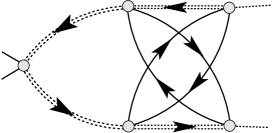
Figure 4: Vertex correction from crossed particle-hole excitations. Such contributions are smaller than the ladder-type corrections by a factor of $\Gamma/V$ and are therefore neglected.

Appendix B Contractions for ${\rm T}^{R(3)}$

In this Appendix, we work out the contraction of Keldysh indices in Eq. (76). There is a total of 9 different non-zero contraction of $ce$ Keldysh-indices, each of which involve renormalization of either zero, one, two or all three vertices. This gives rise to a total of $2^{3}=8$ different types of $pf$ traces, which we need to work out. If the two $ce$ Keldysh indices are different, a vertex contributes with a factor of $\delta_{ab}$ rather than $L_{ab}$. Thus a term with all three vertices renormalized contributes with ${\rm Tr}[{\hat{L}}{\hat{\cal G}}{\hat{L}}{\hat{\cal G}}{\hat{L}}{\hat{\cal G}}]$, whereas a term with no vertices renormalized contributes ${\rm Tr}[\delta{\hat{\cal G}}\delta{\hat{\cal G}}\delta{\hat{\cal G}}]$. Our strategy will be to perform the contraction and the loop-integral over $\omega$ without including the $\lambda$-dependent part of the vertex. After this has been done, it will be a simple matter to include the additional effects of ${{}^{0\!}}{\hat{L}}$, by going through very similar steps once more.

We begin by listing a few useful facts about the relevant matrix products:

$${{}^{0\!}}{\hat{L}}{\hat{\cal G}}=\left(\!\begin{array}[]{cc}{\cal G}^{R}&2{\cal G}^{<}\\ \phi{\cal G}^{R}&2\phi{\cal G}^{<}-{\cal G}^{A}\end{array}\!\right),\,\,\,\,\delta{\hat{\cal G}}=\left(\!\begin{array}[]{cc}{\cal G}^{R}&2{\cal G}^{<}\\ 0&{\cal G}^{A}\end{array}\!\right)$$ (96)

and

$${\rm Tr}\left[\left(\begin{array}[]{cc}a_{1}&b_{1}\\ c_{1}&d_{1}\end{array}\right)\left(\begin{array}[]{cc}a_{2}&b_{2}\\ c_{2}&d_{2}\end{array}\right)\left(\begin{array}[]{cc}a_{3}&b_{3}\\ c_{3}&d_{3}\end{array}\right)\right]=$$ (104)

$$a_{1}a_{2}a_{3}+b_{1}c_{2}a_{3}+a_{1}b_{2}c_{3}+b_{1}d_{2}c_{3}+$$

$$c_{1}a_{2}b_{3}+d_{1}c_{2}b_{3}+c_{1}b_{2}d_{3}+d_{1}d_{2}d_{3}.$$

The lesser component Green function takes the form ${\cal G}^{<}=n_{\lambda}({\cal G}^{A}-{\cal G}^{R})$, and neglecting their slow frequency dependence we may consider the $pf$ distribution functions as constant prefactors. This allows us to expand all terms in products of three Green functions which are either retarded or advanced, and to use rules like ${\cal G}^{R}_{1}{\cal G}^{R}_{2}{\cal G}^{R}_{3}={\cal G}^{A}_{1}{\cal G}^{A}_{2}{\cal G}^{A}_{3}=0$, implied by the subsequent loop integration which can now be performed by closing in the half-plane with no poles. Notice that including the frequency dependence in either factors of $n_{\lambda}$ or $\underline{\Pi}^{ab}$, coming from either propagators or vertices, would render such loop-integrals non-zero. Nevertheless, these contributions will be smaller than the terms which we retain by a factor $\Gamma/V$ and can therefore be neglected. Furthermore, the projection allows us to neglect terms which are proportional to ${\cal G}^{<}{\cal G}^{<}$ or ${\cal G}^{<}{\cal G}^{<}{\cal G}^{<}$.

With these few rules at hand one may work out the following catalog:

$${\rm Tr}\left[({{}^{0\!}}{\hat{L}}{\hat{\cal G}})_{1}({{}^{0\!}}{\hat{L}}{\hat{\cal G}})_{2}({{}^{0\!}}{\hat{L}}{\hat{\cal G}})_{3}\right]=$$

$$\hskip 85.35826pt4n_{\lambda}\left\{\phi_{1}({\cal G}^{R}_{1}{\cal G}^{R}_{2}{\cal G}^{A}_{3}-{\cal G}^{R}_{1}{\cal G}^{A}_{2}{\cal G}^{A}_{3})\right.$$

$$\hskip 102.42992pt+\phi_{2}({\cal G}^{A}_{1}{\cal G}^{R}_{2}{\cal G}^{R}_{3}-{\cal G}^{A}_{1}{\cal G}^{R}_{2}{\cal G}^{A}_{3})$$

$$\left.\hskip 102.42992pt+\phi_{3}({\cal G}^{R}_{1}{\cal G}^{A}_{2}{\cal G}^{R}_{3}-{\cal G}^{A}_{1}{\cal G}^{A}_{2}{\cal G}^{R}_{3})\right\},$$

$${\rm Tr}\left[({{}^{0\!}}{\hat{L}}{\hat{\cal G}})_{1}({{}^{0\!}}{\hat{L}}{\hat{\cal G}})_{2}(\delta{\hat{\cal G}})_{3}\right]=$$

$$\hskip 85.35826pt4n_{\lambda}\left\{\phi_{1}{\cal G}^{R}_{1}{\cal G}^{A}_{2}{\cal G}^{A}_{3}+\phi_{2}{\cal G}^{A}_{1}{\cal G}^{R}_{2}{\cal G}^{R}_{3}\right\},$$

$${\rm Tr}\left[({{}^{0\!}}{\hat{L}}{\hat{\cal G}})_{1}(\delta{\hat{\cal G}})_{2}({{}^{0\!}}{\hat{L}}{\hat{\cal G}})_{3}\right]=$$

$$\hskip 85.35826pt4n_{\lambda}\left\{\phi_{1}{\cal G}^{R}_{1}{\cal G}^{R}_{2}{\cal G}^{A}_{3}+\phi_{3}{\cal G}^{A}_{1}{\cal G}^{A}_{2}{\cal G}^{R}_{3}\right\},$$

$${\rm Tr}\left[(\delta{\hat{\cal G}})_{1}({{}^{0\!}}{\hat{L}}{\hat{\cal G}})_{2}({{}^{0\!}}{\hat{L}}{\hat{\cal G}})_{3}\right]=$$

$$\hskip 85.35826pt4n_{\lambda}\left\{\phi_{2}{\cal G}^{A}_{1}{\cal G}^{R}_{2}{\cal G}^{A}_{3}+\phi_{3}{\cal G}^{R}_{1}{\cal G}^{A}_{2}{\cal G}^{R}_{3}\right\}.$$

The remaining four possibilities all vanish, and we are left with contributions from terms with either two or three vertices renormalized. Working out the loop-integral over $\omega$, we get e.g.

$$\int\!\frac{d\omega}{2\pi}\,\phi_{1}{\cal G}^{R}_{1}{\cal G}^{R}_{2}{\cal G}^{A}_{3} = \int\!\frac{d\omega}{2\pi}\phi(-\varepsilon){\cal G}^{R}(\omega)$$ (106)

$$\hskip 25.60747pt\times{\cal G}^{R}(\omega+\varepsilon^{\prime}){\cal G}^{A}(\omega+\varepsilon)$$

$$= i{\cal G}^{A}_{\Gamma_{2}}(\varepsilon){\cal G}^{A}_{\Gamma}(\varepsilon-\varepsilon^{\prime}),$$

where we have introduced the notation ${\cal G}^{A}_{\Gamma_{2}}(\varepsilon)=(\varepsilon-i\Gamma_{\!s})^{-1}$, and ${\cal G}^{A}_{\Gamma}(\varepsilon)=(\varepsilon-i\Gamma)^{-1}$ for the double-broadened $pf$ Green functions. We see that the vertex corrections serve to replace $\Gamma$ by $\Gamma_{\!s}$ in products of certain internal Green functions, and working out all the integrals, we obtain the following list for the Peierls-channel:

$$\int\!\frac{d\omega}{2\pi}\,\phi_{1}{\cal G}^{R}_{1}{\cal G}^{R}_{2}{\cal G}^{A}_{3} = i{\cal G}^{A}_{\Gamma_{2}}(\varepsilon){\cal G}^{A}_{\Gamma}(\varepsilon-\varepsilon^{\prime}),$$

$$\int\!\frac{d\omega}{2\pi}\,\phi_{1}{\cal G}^{R}_{1}{\cal G}^{A}_{2}{\cal G}^{A}_{3} = -i{\cal G}^{A}_{\Gamma_{2}}(\varepsilon){\cal G}^{A}_{\Gamma}(\varepsilon^{\prime}),$$

$$\int\!\frac{d\omega}{2\pi}\,\phi_{2}{\cal G}^{A}_{1}{\cal G}^{R}_{2}{\cal G}^{R}_{3} = i{\cal G}^{R}_{\Gamma}(\varepsilon){\cal G}^{R}_{\Gamma_{2}}(\varepsilon^{\prime}),$$

$$\int\!\frac{d\omega}{2\pi}\,\phi_{2}{\cal G}^{A}_{1}{\cal G}^{R}_{2}{\cal G}^{A}_{3} = i{\cal G}^{R}_{\Gamma_{2}}(\varepsilon^{\prime}){\cal G}^{A}_{\Gamma}(\varepsilon-\varepsilon^{\prime}),$$

$$\int\!\frac{d\omega}{2\pi}\,\phi_{3}{\cal G}^{R}_{1}{\cal G}^{A}_{2}{\cal G}^{R}_{3} = -i{\cal G}^{A}_{\Gamma}(\varepsilon^{\prime}){\cal G}^{R}_{\Gamma_{2}}(\varepsilon-\varepsilon^{\prime}),$$

$$\int\!\frac{d\omega}{2\pi}\,\phi_{3}{\cal G}^{A}_{1}{\cal G}^{A}_{2}{\cal G}^{R}_{3} = -i{\cal G}^{R}_{\Gamma}(\varepsilon){\cal G}^{R}_{\Gamma_{2}}(\varepsilon-\varepsilon^{\prime}).$$ (107)

As may be seen from Eq. (76), the corresponding products for the Cooper-channel can be obtained from these by the shift of variables $\varepsilon\to-\varepsilon^{\prime}$, and $\varepsilon^{\prime}\to-\varepsilon$. Using the fact that ${\cal G}^{R}(-\varepsilon)=-{\cal G}^{A}(\varepsilon)$, one readily obtains the following list, to be used for the Cooper-channel:

$$\int\!\frac{d\omega}{2\pi}\,\phi_{1}{\cal G}^{R}_{1}{\cal G}^{R}_{2}{\cal G}^{A}_{3} = -i{\cal G}^{R}_{\Gamma_{2}}(\varepsilon^{\prime}){\cal G}^{A}_{\Gamma}(\varepsilon-\varepsilon^{\prime}),$$

$$\int\!\frac{d\omega}{2\pi}\,\phi_{1}{\cal G}^{R}_{1}{\cal G}^{A}_{2}{\cal G}^{A}_{3} = -i{\cal G}^{R}_{\Gamma_{2}}(\varepsilon^{\prime}){\cal G}^{R}_{\Gamma}(\varepsilon),$$

$$\int\!\frac{d\omega}{2\pi}\,\phi_{2}{\cal G}^{A}_{1}{\cal G}^{R}_{2}{\cal G}^{R}_{3} = i{\cal G}^{A}_{\Gamma}(\varepsilon^{\prime}){\cal G}^{A}_{\Gamma_{2}}(\varepsilon),$$

$$\int\!\frac{d\omega}{2\pi}\,\phi_{2}{\cal G}^{A}_{1}{\cal G}^{R}_{2}{\cal G}^{A}_{3} = -i{\cal G}^{A}_{\Gamma_{2}}(\varepsilon){\cal G}^{A}_{\Gamma}(\varepsilon-\varepsilon^{\prime}),$$

$$\int\!\frac{d\omega}{2\pi}\,\phi_{3}{\cal G}^{R}_{1}{\cal G}^{A}_{2}{\cal G}^{R}_{3} = i{\cal G}^{R}_{\Gamma}(\varepsilon){\cal G}^{R}_{\Gamma_{2}}(\varepsilon-\varepsilon^{\prime}),$$

$$\int\!\frac{d\omega}{2\pi}\,\phi_{3}{\cal G}^{A}_{1}{\cal G}^{A}_{2}{\cal G}^{R}_{3} = i{\cal G}^{A}_{\Gamma}(\varepsilon^{\prime}){\cal G}^{R}_{\Gamma_{2}}(\varepsilon-\varepsilon^{\prime}).$$ (108)

It is now straightforward to carry out the contraction of $ce$ Keldysh indices in Eq.(76), and one finds the combination

$$\hskip 8.25128ptG^{R}G^{R}{\rm Tr}\left[({{}^{0\!}}{\hat{L}}{\hat{\cal G}})_{1}({{}^{0\!}}{\hat{L}}{\hat{\cal G}})_{2}({{}^{0\!}}{\hat{L}}{\hat{\cal G}})_{3}\right]$$

$$+G^{K}G^{R}{\rm Tr}\left[({{}^{0\!}}{\hat{L}}{\hat{\cal G}})_{1}({{}^{0\!}}{\hat{L}}{\hat{\cal G}})_{2}(\delta{\hat{\cal G}})_{3}\right]$$

$$+(G^{R}G^{K}+G^{K}G^{A}){\rm Tr}\left[({{}^{0\!}}{\hat{L}}{\hat{\cal G}})_{1}(\delta{\hat{\cal G}})_{2}({{}^{0\!}}{\hat{L}}{\hat{\cal G}})_{3}\right]$$

for the Peierls, and

$$\hskip 8.25128ptG^{R}G^{R}{\rm Tr}\left[({{}^{0\!}}{\hat{L}}{\hat{\cal G}})_{1}({{}^{0\!}}{\hat{L}}{\hat{\cal G}})_{2}({{}^{0\!}}{\hat{L}}{\hat{\cal G}})_{3}\right]$$

$$+G^{K}G^{R}{\rm Tr}\left[({{}^{0\!}}{\hat{L}}{\hat{\cal G}})_{1}({{}^{0\!}}{\hat{L}}{\hat{\cal G}})_{2}(\delta{\hat{\cal G}})_{3}\right]$$

$$+(G^{R}G^{K}+G^{K}G^{A}){\rm Tr}\left[(\delta{\hat{\cal G}})_{1}({{}^{0\!}}{\hat{L}}{\hat{\cal G}})_{2}({{}^{0\!}}{\hat{L}}{\hat{\cal G}})_{3}\right]$$

for the Cooper-channel. Together, the two channels contribute the integral

$${\rm T}_{\alpha\alpha^{\prime}}^{R}{{}^{(3)}}(\Omega)=\frac{3}{16}n_{\lambda}J^{3}_{\alpha\alpha^{\prime\prime}\alpha^{\prime\prime\prime}\alpha^{\prime}}\!\int\!\frac{d\varepsilon}{2\pi}\!\int\!\frac{d\varepsilon^{\prime}}{2\pi}$$

$$\times\left\{G_{\alpha^{\prime\prime}}^{K}(\Omega+\varepsilon)G_{\alpha^{\prime\prime\prime}}^{R}(\Omega+\varepsilon^{\prime}){\cal G}^{A}_{\Gamma_{\!s}}(\varepsilon){\cal G}^{A}_{\Gamma}(\varepsilon^{\prime})\right.$$

$$\hskip 11.38109pt-\left[G_{\alpha^{\prime\prime}}^{R}(\Omega+\varepsilon)G_{\alpha^{\prime\prime\prime}}^{K}(\Omega+\varepsilon^{\prime})\right.$$

$$\left.\left.\hskip 21.33955pt+G_{\alpha^{\prime\prime}}^{K}(\Omega+\varepsilon)G_{\alpha^{\prime\prime\prime}}^{A}(\Omega+\varepsilon^{\prime})\right]{\cal G}^{A}_{\Gamma_{\!s}}(\varepsilon){\cal G}^{A}_{\Gamma}(\varepsilon-\varepsilon^{\prime})\right\}.$$

To include the effects of ${{}^{\lambda\!}}{\hat{L}}$, one may go through the same steps and build up a similar catalog of terms. We have to include all terms with exactly one factor of ${{}^{\lambda\!}}{\hat{L}}$, since terms with two or three factors vanish faster than $\langle Q\rangle_{\lambda}$ under projection. To leading order in $\Gamma/V$, there will still only be contributions with either two or three vertices renormalized. Whereas ${{}^{0\!}}{\hat{L}}$ ended up contributing only with its $21$-entry, $\phi$, this entry is zero in ${{}^{\lambda\!}}{\hat{L}}$ and instead one finds only contributions from its $12$-entry, $\psi$. A typical contribution from the Peierls-channel now takes the form

$$\int\!\!\frac{d\omega}{2\pi}{\rm Tr}\!\left[\!({{}^{0\!}}{\hat{L}}{\hat{\cal G}})_{1}({{}^{\lambda\!}}{\hat{L}}{\hat{\cal G}})_{2}(\delta{\hat{\cal G}})_{3}\right]\!\!\! = \!\!2n_{\lambda}\!\!\int\!\!\frac{d\omega}{2\pi}\phi_{1}{\cal G}^{R}_{1}\psi_{2}{\cal G}^{A}_{2}{\cal G}^{A}_{3}$$

$$= \!\!4n_{\lambda}\frac{i\Gamma_{v}}{\varepsilon^{\prime}-i\Gamma_{\!s}}{\cal G}^{A}_{\Gamma}(\varepsilon^{\prime}){\cal G}^{A}_{\Gamma_{\!s}}(\varepsilon),$$

and a term like this eventually adds up with a similar term from ${\rm Tr}[({{}^{0\!}}{\hat{L}}{\hat{\cal G}})_{1}({{}^{0\!}}{\hat{L}}{\hat{\cal G}})_{2}(\delta{\hat{\cal G}})_{3}]$, having a $1$ in place of the factor of $i\Gamma_{v}/(\varepsilon^{\prime}-i\Gamma_{\!s})$, to contribute $4n_{\lambda}{\cal G}^{A}_{\Gamma_{\!s}}(\varepsilon^{\prime}){\cal G}^{A}_{\Gamma_{\!s}}(\varepsilon)$. Working out the full contribution, from both the Peierls, and the Cooper-channel, one finds that all surviving terms combine in similar ways, and the total effect of including ${{}^{\lambda\!}}{\hat{L}}$ is therefore simply to replace $\Gamma$ by $\Gamma_{\!s}$ in (B). This finally leads to the integral (III) quoted in the main text.

Appendix C Cutting off x-ray edge singularities in the anisotropic Kondo model

In this Appendix, we investigate the anisotropic Kondo model in the case of a vanishing spin-flip coupling ${{}^{\bot\!\!}}J=0$ and finite ${}^{z\!\!}J$. In this limit, certain equilibrium correlation functions are singular at the Fermi energy, they display the so-called X-ray edge singularities whenever the spin is flipped. In the following, we investigate how these singularities are modified in the case of a finite voltage.

Even for ${{}^{\bot\!\!}}J=0$ a finite current is flowing through the system as ${}^{z\!\!}J_{LR}\neq 0$ and we therefore expect that the associated noise will cut off all singularities. Fortunately, a very similar problem has been solved exactly by NgNg96 (see also Refs. Combescot00, and Muzykantskii03, ), who considered the effects of suddenly switching on the tunneling between two (non-interacting) leads.

We will show, that our problem (for ${{}^{\bot\!\!}}J=0$) can be mapped exactly on the one solved by Ng. The fact that this is possible is not obvious as he considered a situation where for times $t<t_{i}$ no current is flowing, whereas in our case the same current passes the dot before and after the spin-flip .

Ng considered the HamiltonianNg96

$$H_{\rm x}=H_{0}(V)+\!\!\!\!\!\sum_{\alpha,\alpha^{\prime},{\bf k},{\bf k}^{\prime},\sigma,\sigma^{\prime}}\!\!\!\!\!V_{\alpha^{\prime}\alpha}\,c^{\dagger}_{\alpha^{\prime}{\bf k}^{\prime}}c_{\alpha{\bf k}}\theta(t_{f}-t)\theta(t-t_{i}),$$ (110)

where $H_{0}(V)=\sum_{\alpha,{\bf k},\sigma}(\varepsilon_{{\bf k}}-\mu_{\alpha})c^{\dagger}_{\alpha{\bf k}\sigma}c_{\alpha{\bf k}\sigma}$ describes the two leads with the bias voltage $V=\mu_{L}-\mu_{R}$. The tunneling between the left and the right lead (and a potential scattering) is switched on for times between $t_{i}$ and $t_{f}$. This generalization of the usual X-ray edge problem to two different Fermi seas was solved by NgNg96 , using a generalization of the method devised by Nozières and De Dominicis for the problem with only a single Fermi sea. He finds that the relevant spectral function exhibits power-law singularities near each of the two Fermi energies in the left and right leads, which are, however, cut off by a voltage induced broadening given in terms of complex phase-shifts (see Ref. Ng96, for details) $\delta_{L/R}$, by

$$\Gamma_{\!{\rm x}}=\frac{V}{2\pi}\text{Im}[\delta_{L}-\delta_{R}].$$ (111)

For ${{}^{\bot\!}}g=0$ and $B=0$, the Kondo Hamiltonian (2) reduces to two separate potential scattering problems for conduction electrons of spin up and down, respectively,

$$H=H_{0}(V)+\!\!\!\!\!\sum_{\alpha,\alpha^{\prime},{\bf k},{\bf k}^{\prime},\sigma,\sigma^{\prime}}\!\!\!\!\!\!\left({{}^{z\!\!}}J_{\alpha^{\prime}\alpha}\,S^{z}/2\right)c^{\dagger}_{\alpha^{\prime}{\bf k}^{\prime}\sigma^{\prime}}\tau^{3}_{\sigma^{\prime}\sigma}c_{\alpha{\bf k}\sigma}.$$ (112)

and we want to study the effect of a single spin-flip, i.e. correlation functions like $\langle S^{-}(t_{f})S^{+}(t_{i})\rangle$ or $\langle[c^{\dagger}_{\alpha^{\prime}\uparrow}(t_{f})S^{-}(t_{f})]\,[S^{+}(t_{i})c_{\alpha\uparrow}(t_{i})]\rangle$ (which is related to the T-matrix). For these correlation functions, the spin points down for $t<t_{i}$, i.e. $S_{z}=-1/2$ and $H(t<t_{i})=H_{i}=H_{0}(V)-\frac{1}{4}\sum_{\alpha,\alpha^{\prime},{\bf k},{\bf k}^{\prime},\sigma,\sigma^{\prime}}{{}^{z\!\!}}J_{\alpha^{\prime}\alpha}c^{\dagger}_{\alpha^{\prime}{\bf k}^{\prime}\sigma^{\prime}}\tau^{3}_{\sigma^{\prime}\sigma}c_{\alpha{\bf k}\sigma}$. To map Eq. (112) onto Eq. (110) we note that $S_{z}=1/2$ for $t_{i}<t<t_{f}$ and therefore

$$H=H_{i}+\!\!\!\!\!\sum_{\alpha,\alpha^{\prime},{\bf k},{\bf k}^{\prime},\sigma,\sigma^{\prime}}\!\!\!\!\!\!({{}^{z\!\!}}J_{\alpha^{\prime}\alpha}/2)c^{\dagger}_{\alpha^{\prime}{\bf k}^{\prime}\sigma^{\prime}}\tau^{3}_{\sigma^{\prime}\sigma}c_{\alpha{\bf k}\sigma}\theta(t_{f}-t)\theta(t-t_{i}).$$ (113)

$H_{i}$ can easily be diagonalized in terms of scattering states. Scattering states coming from the left (right) lead are occupied according to the left (right) chemical potential and therefore, (113) takes the form (110) when rewritten in terms of those scattering states.

To determine the scattering states of $H_{i}$, we represent for convenience the two semi-infinite leads by infinite chiral wires of right-movers. In this representation, the scattering wave-functions $\Phi^{\alpha^{\prime}\alpha}_{k\sigma}(x)$ describe the amplitude of plane waves coming from lead $\alpha$

$$\Phi^{\alpha^{\prime}\!\alpha}_{k\sigma}(x)=\left[\theta(-x)\delta_{\alpha^{\prime}\alpha}+\theta(x)S_{\alpha^{\prime}\!\alpha}\right]e^{ikx},$$ (114)

where $x<0$ ($x>0$) refers to incoming (outgoing) waves in lead $\alpha^{\prime}$. The scattering matrix $S_{\alpha^{\prime}\!\alpha}$ is determined from the Schrödinger equation

$$\left[-iv_{F}\partial_{x}\delta_{\alpha^{\prime}\alpha^{\prime\prime}}-\frac{\sigma}{4}{{}^{z\!\!}}J_{\alpha^{\prime}\alpha^{\prime\prime}}\delta(x)\right]\Phi_{k\sigma}^{\alpha^{\prime\prime}\!\alpha}(x)=\varepsilon\,\Phi_{k\sigma}^{\alpha^{\prime}\!\alpha}(x),$$ (115)

and regularizing the delta-function by using $\theta(0)=1/2$ we obtain

$$S_{LL} = \frac{1-({{}^{z}\!\!\,g}_{LR}^{2}-{{}^{z}\!\!\,g}_{LL}{{}^{z}\!\!\,g}_{RR})/64+i\sigma({{}^{z}\!\!\,g}_{LL}-{{}^{z}\!\!\,g}_{RR})/8}{1+({{}^{z}\!\!\,g}_{LR}^{2}-{{}^{z}\!\!\,g}_{LL}{{}^{z}\!\!\,g}_{RR})/64-i\sigma({{}^{z}\!\!\,g}_{LL}+{{}^{z}\!\!\,g}_{RR})/8},$$

$$S_{LR} = \frac{{{}^{z}\!\!\,g}_{LR}2i\sigma/8}{1+({{}^{z}\!\!\,g}_{LR}^{2}-{{}^{z}\!\!\,g}_{LL}{{}^{z}\!\!\,g}_{RR})/64-i\sigma({{}^{z}\!\!\,g}_{LL}+{{}^{z}\!\!\,g}_{RR})/8},$$

with ${{}^{z}\!\!\,g}_{\alpha\alpha^{\prime}}=N(0)\,{{}^{z\!\!}}J_{\alpha\alpha^{\prime}}$ and $N(0)=1/v_{F}$.

Rewriting Eq. (113) in terms of these scattering states, we can read off the potential in Eq. (110)

$$V_{\alpha^{\prime}\alpha}=\frac{1}{2}\sum_{\beta\beta^{\prime}}\,{{}^{z\!\!}}J_{\beta^{\prime}\beta}\,[\Phi_{\sigma}^{\beta^{\prime}\alpha^{\prime}}(0)]^{\ast}\,\Phi_{\sigma}^{\beta\alpha}(0).$$ (117)

Using this formula and the results by NgNg96 , one can easily work out the relevant correlation functions when taking into account that the spin-up and spin-down problems separate. The corresponding correlation functions are therefore multiplied in the time-domain and convoluted as a function of frequency. We will not display the rather lengthy formulas, but only note that all divergences close to the two Fermi levels are cut off by the appropriate relaxation rates (111) [the rates for spin-up and spin-down add as $e^{-\Gamma_{\uparrow}t}e^{-\Gamma_{\downarrow}t}=e^{-(\Gamma_{\uparrow}+\Gamma_{\downarrow})t}$].

To make contact with our perturbative results, we will now consider the case of small ${}^{z\!\!}J$. In this limit $V_{\alpha^{\prime}\alpha}\approx\,{{}^{z\!\!}}J_{\beta^{\prime}\beta}/2$. Inserting this into Eqs. (11d) and (11f) of Ref. Ng96, , determining the complex phase-shifts $\delta_{L/R}$, expanding the result to leading order in $V_{\alpha^{\prime}\alpha}$ and adding spin-up and spin-down contributions, we find

$$\Gamma_{\!{\rm x}}=\frac{\pi}{2}V|{{}^{z\!}}g_{LR}|^{2},$$ (118)

which coincides with our $\Gamma_{2}=1/T_{2}$ in Eq. (91), in the limit of ${{}^{\bot\!}}g\to 0$. Note that the first logarithm in Eq. (IV) arises from a diagram with $S_{z}$ at an external vertex. Therefore the corresponding correlator is not of the X-ray edge form discussed in this Appendix.

References

(1) A. C. Hewson, The Kondo Problem to Heavy
Fermions, Cambridge University Press (1993).
(2)D. Goldhaber-Gordon, Hadas Shtrikman, D. Mahalu,
David Abusch-Magder, U. Meirav and M. A. Kastner, Nature 391,
156 (1998); S. M. Cronenwett, T. H. Oosterkamp and L. P.
Kouwenhoven, Science 281, 540 (1998); W. G. van der Wiel, S.
De Franceschi, T. Fujisawa, J. M. Elzerman, S. Tarucha and L. P.
Kouwenhoven, Science 289, 2105 (2000); J. Nygård, D. H.
Cobden and P. E. Lindelof, Nature 408, 342 (2000).
(3)J. Korringa, Physica 16, 601 (1950).
(4)Y.-L. Wang and D. J. Scalapino, Phys. Rev. 117,
734 (1968).
(5) H. Schoeller and J. König, Phys. Rev. Lett.
84, 3686 (2000); M. Keil, ph.d. thesis, Aachen (2002); H.
Schoeller, Lect.Notes Phys. 544, 137 (2000).
(6)A. Rosch, J. Paaske, J. Kroha and P. Wölfle, Phys.
Rev. Lett. 90, 076804 (2003)
(7)E. L. Wolf and D. L. Losee, Phys. Rev. Lett. 23,
1457 (1969).
(9)J. Appelbaum and L. Y. Shen Phys. Rev. B 5,
544 (1972).
(10)S. Bermon, D. E. Paraskevopoulos and P. M. Tedrow,
Phys. Rev. B 17, 2110 (1978).
(11)Y. Meir, N. S. Wingreen and P. A. Lee, Phys. Rev.
Lett. 70, 2601 (1993); N. S. Wingreen and Y. Meir, Phys. Rev.
B 49, 11040 (1994).
(12)A. Rosch, J. Kroha and P. Wölfle, Phys. Rev.
Lett. 87, 156802 (2001).
(13)A. Kaminski, Yu. V. Nazarov and L. I. Glazman,
Phys. Rev. Lett 83, 384 (1999); Phys. Rev. B 62, 8154
(2000).
(14) P. Coleman, C. Hooley and O. Parcollet, Phys. Rev.
Lett. 86, 4088 (2001); P. Coleman and W. Mao,
cond-mat/0203001.
(15) M. N. Kiselev, K. Kikoin, and L. W. Molenkamp
Phys. Rev. B 68, 155323 (2003); JETP Letters 77, 366
(2003).
(16)W. Mao, P. Coleman, C. Hooley and D. Langreth, Phys.
Rev. Lett. 91, 207203 (2003).
(17)A. Shnirman and Y. Makhlin, Phys. Rev. Lett. 91,
207204 (2003).
(18)J. Paaske, A. Rosch, and P. Wölfle,
cond-mat/0307365.
(19)J. Rammer and H. Smith, Rev. Mod. Phys. 58,
323 (1986).
(20)M. B. Walker, Phys. Rev. 176, 432 (1968);
Phys. Rev. B 1, 3690 (1970).
(21) W. Götze and P. Wölfle, JLTP 5, 575
(1971).
(22)D. Langreth and J. Wilkins, Phys. Rev. B 6,
3189 (1972).
(23)D. C. Langreth in Linear and Nonlinear
Electron Transport in Solids, eds. J. T. Devreese and E. Van
Doren (Plenum, New York, 1976); H. Haug and A. -P. Jauho, Quantum Kinetics in Transport and Optics of Semiconductors,
Springer-Verlag (Berlin, 1996).
(24) A. Rosch, T. A. Costi, J. Paaske, P. Wölfle, Phys.
Rev. B 68, 014430 (2003).
(25) S. De Franceschi, R. Hanson, W. G. van der
Wiel, J. M. Elzerman, J. J. Wijpkema, T. Fujisawa, S. Tarucha, and
L. P. Kouwenhoven, Phys. Rev. Lett. 89, 156801 (2002).