Green’s function theory for a magnetic impurity layer in a ferromagnetic Ising film with transverse field

Abstract

A Green’s function formalism is used to calculate the spectrum of localized modes of an impurity layer implanted within a ferromagnetic thin film. The equations of motion for the Green’s functions are determined in the framework of the Ising model in a transverse field. We show that depending on the thickness, exchange and effective field parameters, there is a “crossover” effect between the surface modes and impurity localized modes. For thicker films the results show that the degeneracy of the surface modes can be lifted by the presence of an impurity layer.

, , ,

1 Introduction

The spectrum of elementary excitations in solids is known to be modified by the presence of surfaces in the medium in which they propagate. This occurs because an interface breaks the translational symmetry of the medium and can also modify the microscopic scheme of interactions due to surface reconstruction effects. The modifications of the spectrum can be signaled by the appearance of surface localized modes, besides the volume excitations. The translational symmetry of a crystal can also be broken by the presence of defects or impurities in the lattice, and localized excitations may result.

Localized excitations of magnetic media have been widely studied, theoretically as well as experimentally [1] and several models have been proposed to elucidate the dynamics of surface modes in a variety of magnetic systems. Among these models, the transverse Ising model has been shown to give a good theoretical description of real materials with anisotropic exchange (e.g., CoCs₃Cl₅ and DyPO₄), of materials in which the crystal field ground state is a singlet [2], and has also been employed as a pseudo-spin model for hydrogen-bonded ferroelectric materials [3]. Previous calculations have obtained the spin wave (SW) spectrum of Ising ferromagnets in a transverse external field for semi-infinite systems [4] and films [5]. These results were obtained for ideal media, i.e. structures without defects or impurities. Studies [6, 7, 8, 9, 10] concerning excitations of semi-infinite systems described by the transverse Ising model have predicted the existence of localized SW modes, as well as bulk SW.

Within the quasi-particle approximation, the effect of a localized perturbation in a periodic structure can be worked out exactly using Green’s functions techniques. These techniques have been extensively used to calculate the impurity modes in infinite and semi-infinite Heisenberg ferromagnets and antiferromagnets [11, 12].

The purpose of this paper is to present the first calculation of the SW spectrum of a thin ferromagnetic film with an impurity layer in the framework of an Ising model in a transverse field. Dispersion relations for the bulk, surface and impurity SW modes are obtained by finding the poles of the Green’s functions associated with the spin operators of each layer in the film. This calculation generalizes a previous study of the spin dynamics of an impurity layer in a semi-infinite ferromagnet, presented in Ref. [10].

2 Green’s function formalism

Let us consider a retarded Green’s function, defined in terms of two time-dependent operators $A(t)$ and $B(t)$, in the Heisenberg picture, as:

$$G_{r}(t-t^{\prime})=\langle\langle A(t);B(t^{\prime})\rangle\rangle,$$ (1)

which, in frequency representation, can be shown to satisfy the equation of motion [13],

$$\omega\left\langle\left\langle A;B\right\rangle\right\rangle_{\omega}=\frac{1}{2\pi}\left\langle\left[A,B\right]\right\rangle+\left\langle\left\langle\left[A,{\mathcal{H}}\right];B\right\rangle\right\rangle_{\omega},$$ (2)

where $\omega$ is a frequency label, and ${\mathcal{H}}$ is the Hamiltonian of the system. In the present case we employ the Ising Hamiltonian in a transverse field

$${\mathcal{H}}=-\frac{1}{2}\sum_{<i,j>}J_{ij}S_{i}^{z}S_{j}^{z}-h\sum_{i}S_{i}^{x},$$ (3)

where $S_{i}^{\alpha}(\alpha=x,y,z)$ is a spin operator component at site $i$, $h$ is the applied transverse magnetic field, taken as $h_{S}$ in the surface and $h_{I}$ in the impurity layer, and $\ J_{ij}$ is the exchange coupling between nearest-neighbor sites $i$ and $j$. The exchange parameter is taken as $J$ in the bulk region, as $J_{S}$ in the surface and as $J_{I}$ in the impurity layer. The exchange coupling between a spin in the surface layer or in the impurity layer and a spin in the adjacent bulk layers is assumed to be $J^{\prime}_{S}$ and $J^{\prime}_{I}$, respectively. In the special case where the impurity layer and the surface are adjacent we use $J_{SI}$ as the exchange interaction. Next, we construct the equation-of-motion

$$\omega\left\langle\left\langle S_{l}^{\alpha};S_{m}^{\beta}\right\rangle\right\rangle_{\omega}= \frac{1}{2\pi}\left\langle\left[S_{l}^{\alpha},S_{m}^{\beta}\right]\right\rangle+\qquad\qquad$$

$$\left\langle\left\langle\left[S_{l}^{\alpha},{\mathcal{H}}\right];S_{m}^{\beta}\right\rangle\right\rangle_{\omega}.$$

where $l$ and $m$ are labels assigned to each lattice site. Thus we obtain an infinite chain of coupled equations, which can then be decoupled using the Random Phase Approximation [14],

$$\left\langle\left\langle S_{l}^{\alpha}S_{j}^{\gamma};S_{m}^{\beta}\right\rangle\right\rangle_{\omega}\approx \left\langle S_{l}^{\alpha}\right\rangle\left\langle\left\langle S_{j}^{\gamma};S_{m}^{\beta}\right\rangle\right\rangle_{\omega}+\qquad\qquad$$

$$\left\langle S_{j}^{\gamma}\right\rangle\left\langle\left\langle S_{l}^{\alpha};S_{m}^{\beta}\right\rangle\right\rangle_{\omega},$$

where $l\neq j$. Using this approximation and inserting the Hamiltonian Eq. (3) into the equation of motion Eq. (2), we obtain

$$A(\omega)\langle\langle S_{l}^{z};S_{m}^{z}\rangle\rangle_{\omega}= hR_{l}^{x}\frac{\delta_{lm}}{2\pi}-\qquad\qquad\qquad\qquad$$

$$\qquad hR_{l}^{x}\sum_{j}J_{lj}\left\langle\left\langle S_{j}^{z};S_{m}^{z}\right\rangle\right\rangle_{\omega},$$

where

$$A(\omega)=\left\{\omega^{2}-\sum_{j}J_{lj}R_{j}^{z}\left(\sum_{i}J_{il}R_{i}^{z}\right)-h^{2}\right\},$$

with $R_{l}^{z}=\left\langle S_{l}^{z}\right\rangle$ and $R_{l}^{x}=\left\langle S_{l}^{x}\right\rangle$.

Equation (6) may be solved to obtain the spin-dependent Green’s functions at any temperature. In this work we focus on the paramagnetic phase, at $T\geq T_{c}$, where $T_{c}$ is the Curie temperature of the ferromagnet. In this regime, due to the absence of net magnetization, we have $\left\langle S_{j}^{z}\right\rangle=0$. For spin S=1/2, we use the static spin average in the $x$ direction calculated from the mean-field theory[3]

$$R^{x}_{\ell}=\frac{1}{2}\tanh\left(\frac{h_{\ell}}{2k_{B}T}\right),$$ (7)

where, depending on the site layer , the index $\ell$ stands for $S,B,I$, for surface, bulk, and impurity layers, respectively and $k_{B}$ is Boltzmann’s constant. After some straightforward algebra, the Green’s function is found as:

$$G_{nn\prime}=\frac{1}{2\pi}\left[\frac{hR^{x}_{\ell}}{\omega^{2}-h^{2}+4hR^{x}_{\ell}J\gamma({\bf{q}_{\parallel}})}\right],$$ (8)

where $n$ and $n^{\prime}$ are layer indices and $\gamma({\bf{q}_{\parallel}})$ is the structure factor, given by,

$$\gamma({\bf{q}_{\parallel}})=\frac{1}{2}\bigl{[}\cos(q_{x}a)+\cos(q_{y}a)\bigr{]}.$$ (9)

Some mathematical techniques, including general recursive algorithms for layered systems, are available to solve these equations. Here we obtain explicit results using an approach analogous to earlier calculations for pure ferromagnets [8]. We write the coupled equations in a matrix form

$$({\bf A}_{0}+{\bf\Delta}){\bf G}=-\Bigl{(}\frac{1}{2\pi J}\Bigr{)}\bf{I}$$ (10)

where ${\bf A}_{0}$ is a $N\times N$ tridiagonal matrix, with $N$ being the total number of layers in the film. The elements of ${\bf A}_{0}$ are defined by

$$[A_{0}]_{l,m}=d\;\delta_{l,m}-(\delta_{l-1,m}+\delta_{l+1,m}),$$ (11)

which represents the system without impurities, and ${\bf\Delta}$ is a $N\times N$ matrix containing the information regarding the perturbing effects of both the surfaces and the impurities, with elements given by

$$\Delta_{1,1}=\Delta_{N,N}=\Delta_{S}$$ (12)

$$\Delta_{1,2}=\Delta_{2,1}=\Delta_{N,N-1}=\Delta_{N-1,N}=\Delta_{SB}$$

$$\Delta_{l,l}=\Delta_{I}$$

$$\Delta_{l+1,l}=\Delta_{l-1,l}=\Delta_{l,l+1}=\Delta_{l,l-1}=\Delta_{IB},$$

where the index $l$ refers to the impurity layer, and the other elements are set to zero. The parameter $d$ is defined by:

$$d=-\frac{\omega^{2}-h^{2}+4hR^{x}_{B}J\gamma({\bf{q}_{\parallel}})}{hR^{x}_{B}J}.$$ (13)

The parameters $\Delta_{S}$, $\Delta_{SB}$, $\Delta_{I}$ and $\Delta_{IB}$, which depend on the surface and on the impurity are

$$\Delta_{S}=-\frac{\omega^{2}-h_{S}^{2}+4h_{S}R_{S}^{x}J_{S}\gamma({\bf{q}_{\parallel}})}{h_{S}R_{S}^{x}J}-d$$ (14)

$$\Delta_{SB}=-\frac{J-J_{S}}{J}$$ (15)

$$\Delta_{I}=-\frac{\omega^{2}-h_{I}^{2}+4h_{I}R_{I}^{x}J_{I}\gamma({\bf{q}_{\parallel}})}{h_{I}R_{I}^{x}J}-d$$ (16)

and,

$$\Delta_{IB}=-\frac{J-J_{I}^{\prime}}{J}.$$ (17)

Finally, we rewrite the Green’s function in matrix form:

$${\bf G}=-\left(\frac{1}{2\pi J}\right)\left[({\bf I}+{\bf A}_{0}^{-1}{\bf\Delta})^{-1}\right]{\bf A}_{0}^{-1}.$$ (18)

The inverse of the tridiagonal matrix ${\bf A}_{0}$ can be found in the literature.

3 Surface and impurity modes

In order to calculate the dispersion relations of the localized SW modes, one has to find the poles of the Green’s function Eq.(18). These are obtained by solving the determinantal equation [8]

$$\det({\bf I}+{{\bf A}_{0}}^{-1}{\bf\Delta})=0.$$ (19)

The elements of the inverse matrix ${{\bf A}_{0}}^{-1}$ involve a factor $x$, which is defined in terms of the diagonal element of ${\bf A}_{0}$ as

$$d=x+x^{-1}.$$ (20)

Solutions of Eq. (19) involving $|x|=1$ give us the frequencies of the quantized bulk modes. Such solutions correspond to $x=\exp(i\alpha a)$, where $\alpha$ is a set of real discrete values $(0\leq\alpha\leq\pi)$ which depends on the film thickness and can be obtained from the determinantal equation. Therefore, from Eq.(13) we obtain the relationship:

$$\omega_{B}({\bf{q}_{\parallel}},\alpha)= \{h^{2}-2hR^{x}J\gamma[\cos(q_{x}a)+\qquad\qquad$$

$$\qquad\cos(q_{y}a)+\cos(\alpha a)]\}^{\frac{1}{2}}$$

where $\bf{q}_{\parallel}$ is a two-dimensional wave vector.

We are interested in understanding how the surface and localized impurity modes affect each other. In order to do that, we start our analysis by considering a film with 5 layers, where the first layer is taken as the impure one. In this case, the $\Delta$ matrix can be expressed as:

$$\mathbf{\Delta}^{(5)}=\left(\begin{array}[]{ccccc}\Delta_{I}&\Delta_{IB}&0&0&0\\ \Delta_{IB}&0&0&0&0\\ 0&0&0&0&0\\ 0&0&0&0&\Delta_{S}\\ 0&0&0&\Delta_{S}&\Delta_{1}\end{array}\right).$$ (22)

Figure 1: SW dispersion for a thin ferromagnetic film with an impurity layer at the surface, for $J_{I}=1.5J$. The bulk band is represented by the shaded region. Parameters in the text.

Figure 1 shows a plot of frequency as a function of wave vector $q_{x}a/\pi$, where $q_{y}=0$, for an impurity layer located on the surface of a 5 layers film, with the parameters: $R^{x}=0.25$, $J_{I}=1.5J$, $J_{I}^{{}^{\prime}}=1.25J$, $J_{S}=1.5J$, $h_{S}=1.5h$, $h_{I}=1.35h$ and $J_{SI}=1.0J$. The shaded area in the graph corresponds to the region containing the volume modes of the infinite case. One can observe the presence of two surface branches located above the bulk region. The branches are associated with the two surfaces of the film, one of these being the impurity layer. The figure also shows a “crossover” effect (with mode repulsion) between the surface and the surface impurity modes at $q_{x}\approx 0.22$. The existence of this crossover is dependent on the strength of the impurity exchange, as can be seen in the next graph. The results in Fig. 2 were calculated for a smaller value for the exchange constant in the impurity layer, namely $J_{I}=0.5J$, with the remaining parameters being the same as those in Fig. 1. The graph shows two localized SW branches. The lower frequency mode does not display any shift in relation to the result in Fig. 1. On the other hand, the upper SW branch shows a significant shift in comparison with the corresponding branch in Fig. 1. Thus, we may associate the lower frequency branch with the pure surface of the film, whereas the upper branch can be associated with the surface impurity layer mode, since the shift occurs as a direct consequence of the smaller value of $J_{I}$. Also, due to the frequency shift, no mode repulsion effects are found.

Let us now consider the situation in which the impurity layer is located in the interior of the film. Results for this case are shown in Fig. $3$, for a $5$ layer film, in which the impurity layer corresponds to the $3$rd layer of the film. The $\Delta$ matrix for this configuration is:

$$\mathbf{\Delta}^{(5)}=\left(\begin{array}[]{ccccc}\Delta_{1}&\Delta_{S}&0&0&0\\ \Delta_{S}&0&\Delta_{IB}&0&0\\ 0&\Delta_{IB}&\Delta_{I}&\Delta_{IB}&0\\ 0&0&\Delta_{IB}&0&\Delta_{S}\\ 0&0&0&\Delta_{S}&\Delta_{1}\end{array}\right).$$ (23)

The SW frequencies are obtained following a procedure similar to the previous case. The parameters are $h_{I}=1.45h$, $J_{I}=1.5J$, $J_{I}^{{}^{\prime}}=1.25J$, $h_{S}=1.35h$, $J_{S}=0.5J$, $J_{S}^{{}^{\prime}}=1.0J$, $J_{SI}=1.0J$, with $R^{x}=0.25$. The plot shows three coupled modes. For small wave vectors, there are two degenerate frequency branches related to the surfaces, as well as a lower frequency one (impurity mode). As the wave vector increases, the degeneracy is lifted. In the range $0.5\pi<q_{x}a<0.7\pi$, there are three distinct modes. That happens as a consequence of a double crossover, due to the mixing of the surface and impurity modes. For larger values of $q_{x}$, the surface modes are again degenerate.

Figure $4$ shows a graph of the frequencies of localized SW modes as a function of the effective field $h_{I}$ in the impurity layer. We used a film with the same parameters as the one discussed in Fig. 3. Results are shown for three different values of in-plane wave vector, namely $q_{x}a=0.01\pi$ (solid line), $q_{x}a=0.5\pi$ (long-dashed line) and $q_{x}a=1.0\pi$ (dotted line). In contrast with the semi-infinite case presented in Ref. [10], the graph displays a rich spectrum of localized modes. The discontinuity in the graph is a consequence of the merging of some of the modes with the bulk band for certain values of $h_{I}$. For each value of wave vector, the graph shows two different behaviors of the localized SW branches: some branches display a strong dependence on $h_{I}$, whereas the remaining branches are not noticeably influenced by a varying field, except at larger values of $h_{I}$, where mode mixing effects are observed. These contrasting behaviors reflect the distinct nature of these modes, with the impurity modes being associated with the branch that is strongly influenced by the $h_{I}$ field. These impurity modes have acoustic nature for small values of $h_{I}$. As the effective field is increased, the impurity mode merges with the bulk band and eventually reappears as an optical mode. For the parameters used in this calculation, the surface modes are found above the bulk band.

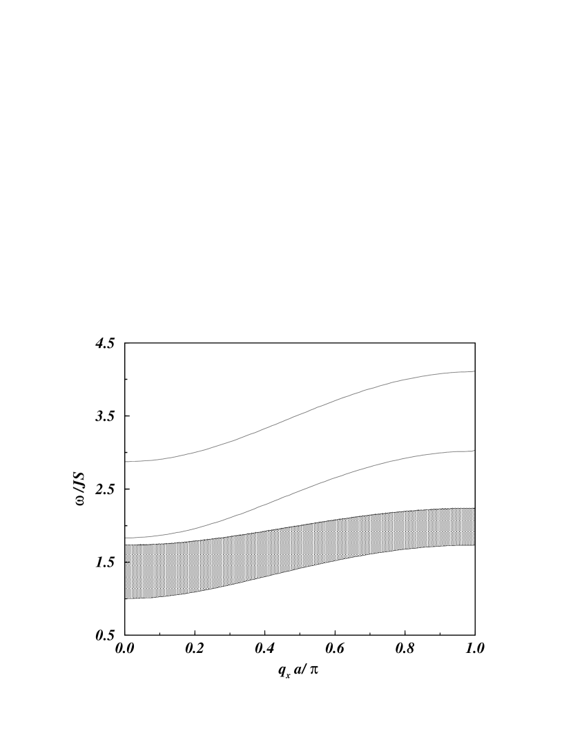
Figure 2: SW dispersion, for a system similar to the film of Fig. 1, with $J_{I}=0.5J$.

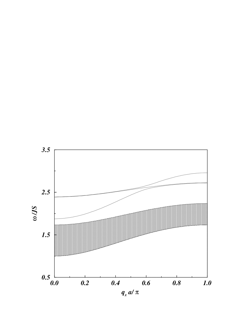
Figure 3: SW dispersion, for an impurity layer in the interior of the film, corresponding to the third atomic layer. The bulk band is represented by the shaded region. Parameters in the text.

Figure 4: Localized SW frequencies as a function of impurity magnetic field for three values of wave vector. Parameters in the text.

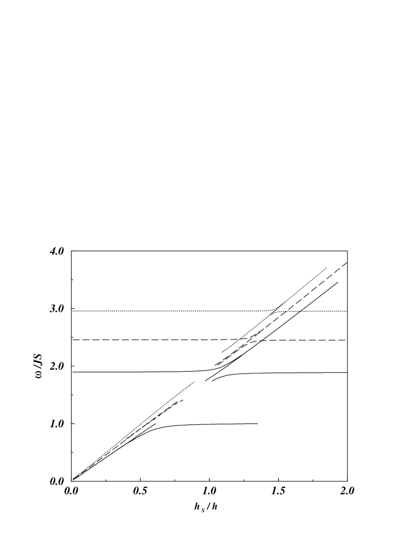
Figure 5: Localized SW frequencies as a function of surface field for three values of wave vector (solid curve, $q_{x}a/\pi=0.5$; long-dashed curve, $q_{x}a/\pi=0.01$ and dot-dashed curve, $q_{x}a/\pi=1.0$). The impurity layer corresponds to the 3rd layer of a 5 layers film.

This difference in behavior is also evident in the results of Fig. $5$, which shows localized SW frequencies as a function of the effective surface field $h_{S}$, for the same wave vector values as in the previous results and $h_{I}/h=1.45$. The graph shows the influence of $h_{S}$ on the surface modes. For small values of this effective field, the surface modes are degenerate and have acoustic behavior. On the other hand, the impurity modes are not affected by the variation of $h_{S}$. As the field is increased, the surface modes merge with the bulk band, and an acoustic impurity mode is observed. Mode mixing effects are also found. For larger values of $h_{S}$, surface modes are found above the bulk band and there are two impurity modes: one optical branch, and one acoustical.

4 Conclusions

In summary, we developed a Green’s Function formalism for calculating the SW spectrum of a ferromagnetic thin film with an impurity layer, in the framework of the transverse Ising Model, using the RPA to obtain equations of motion for the bulk, surface and impurity SW modes. We calculated the Green’s functions analytically through an inhomogeneous matrix equation in a closed form. The formalism can be applied for any temperature, and we obtained explicit solutions for $T\geq T_{c}$. The results showed the effect of the exchange coupling between spin sites in the impurity layer on the localized modes of a film in which the impurity layers correspond to one of the surfaces. We also obtained results for the effect of the position of the impurity layer in the film. We found that the placement of the impure layer has a strong effect on the spectrum of localized modes. In all cases, we observed strong mode mixing effects between localized impurity and surface modes. In addition, we calculated the localized SW frequencies as functions of the effective fields $h_{I}$ and $h_{S}$. This allowed us to analyze the nature of the modes, by observing the response of the frequency branches to the variation of the effective fields. In the limit $N\rightarrow\infty$, the results agree with previous calculations for semi-infinite systems [10]. This formalism can also be applied to obtain the spectral intensities of the bulk and localized SW modes. Currently, we are extending the formalism in order to include the effects of localized impurities in thin films.

The authors gratefully acknowledge partial support the Brazilian agency CNPq.

References

- [1] M. G. Cottam and D. R. Tilley, Introduction to Surface and Superlattice Excitations, Cambridge University Press, Cambridge (1989).
- [2] Y. L. Wong, B. Cooper, Phys. Rev. 172, 539 (1968).
- [3] R. Blinc, B. Zeks, J. Phys. C17, 1973 (1984).
- [4] B. A. Shiwai, M. G. Cottam, Phys. Stat. Sol. B134, 597 (1986).
- [5] M. G. Cottam and D. E. Kontos, J. Phys. C13, 2945 (1980).
- [6] Wax N., Selected Papers on Noise and Stochastic Processes (New York: Dover Publications-1954).
- [7] Dewames R. E. and Wolfram T., Phys. Rev. 185, 720 (1969).
- [8] M. G. Cottam, J. Phys. C9, 2121 (1976).
- [9] M. G. Cottam, D. R. Tilley, and B. Zeks, J. Phys. C 17, 1793 (1984).
- [10] R. N. Costa Filho, U.M.S. Costa, M.G. Cottam, J. Mag. and Mag. 213, 195-200 (2000).
- [11] R. A Cowley, W. J. L. Buyers, Rev. Mod. Phys. 44, 406 (1991).
- [12] N. N. Chen, M. G. Cottam, Phys. Rev. B45, 266 (1992).
- [13] D. N. Zubarev, Soviet Phys. Uspkhi 3, 320 (1960).
- [14] F. Keffer, ”Spin Waves”, in Handbuch der Physik,vol. XVIII/B, ed. S. Flüge, Springer-Verlag, Berlin, 1994.