Approach to asymptotic behavior in the dynamics of the trapping reaction

Abstract

We consider the trapping reaction $A+B\to B$ in space dimension $d=1$, where the $A$ and $B$ particles have diffusion constants $D_{A}$, $D_{B}$ respectively. We calculate the probability, $Q(t)$, that a given $A$ particle has not yet reacted at time $t$. Exploiting a recent formulation in which the $B$ particles are eliminated from the problem we find, for $t\to\infty$, $Q(t)\sim\exp[-(4/\sqrt{\pi})(\rho^{2}D_{B}t)^{1/2}-(C\rho^{2}D_{A}t)^{1/3}+\cdots]$, where $\rho$ is the density of $B$ particles and $C\propto D_{A}/D_{B}$ for $D_{A}/D_{B}\ll 1$.

I Introduction

The trapping reaction, $A+B\to B$, where $A$ and $B$ are diffusing particles with diffusion constants $D_{A}$ and $D_{B}$ respectively, has seen a resurgence of interest in the last few years MG ; BB ; BB2 ; BMB ; OBCM ; MOBC . The problem is related to the two-species annihilation reaction TW , $A+B\to 0$, in the case where the initial particle densities satisfy $\rho_{A}(0)<\rho_{B}(0)$. In the long-time limit $\rho_{A}(t)\ll\rho_{B}(t)$, and to study the asymptotic decay of the $A$-particle density it suffices to study the survival probability, $Q(t)$, of a single $A$ particle diffusing in a sea of $B$ particles. In this limit, the two-species annihilation reaction is equivalent to the trapping reaction. As the initial condition, the $B$-particles are taken to be randomly distributed in space with uniform density $\rho$, i.e. the probability to find a $B$-particle in a volume element $dV$ is $\rho dV$.

The problem of determining the asymptotic behavior of $Q(t)$ has only recently been solved BB ; BB2 . The solution is limited to space dimensions $d\leq 2$. The asymptotic form of the solution has been known for some time BL . The $A$-particle survival probability is given by

$$Q(t)\sim\left\{\begin{array}[]{ll}\exp(-\lambda_{d}t^{d/2}),&\ \ d<2\\ \exp(-\lambda_{2}t/\ln t),&\ \ d=2\\ \exp(-\lambda_{d}t),&\ \ d>2\\ \end{array}\right.$$ (1)

but the values of the constants $\lambda_{d}$ were not known. In refs. BB ; BB2 , these were determined for $d\leq 2$ by deriving upper and lower bounds on $Q(t)$ and showing that they pinch as $t\to\infty$. The restriction to $d\leq 2$ is a consequence of the recurrence properties of random walks. For $d<2$, all particles can be treated as zero-size points. As a consequence, the combinations $\rho(D_{B}t)^{d/2}$ and $D_{A}/D_{B}$ are the only dimensionless quantities in the theory. A key result of BB ; BB2 is that the coefficients $\lambda_{d}$ in Eq. (1) are independent of $D_{A}$ for $d\leq 2$, and therefore have the form $\lambda_{d}=a_{d}\,\rho D_{B}^{d/2}$, where the quantities $a_{d}$ are pure numbers. The result of BB ; BB2 is

$$a_{d}=\left\{\begin{array}[]{ll}(4\pi)^{d/2}\,(2/\pi d)\sin(\pi d/2),&\ \ d<2\\ 4\pi,&\ \ d=2\\ \end{array}\right.$$ (2)

For $d=2$, the $A$-particle has to be given a non-zero size, but this size only enters as a cut-off in the logarithm in Eq. (1).

Although these results are asymptotically exact, numerical studies MG ; BB2 show that the asymptotic regime is not reached, either in $d=1$ or $d=2$, after any time accessible to simulation, even using sophisticated simulation methods MG that allow values of $Q(t)$ as small as $10^{-70}$ to be achieved. It is natural, therefore, to try to calculate the leading correction to the asymptotic behavior. This is the principal aim of this paper. It should be stated at the outset that this is a very challenging problem, and we have obtained concrete results only in the limit $D_{A}\ll D_{B}$.

The starting point of our approach is an equation, first presented in BMB , that implicitly determines the survival probability of the $A$-particle for a given $A$-particle trajectory, averaged over all the $B$-particle trajectories and $B$-particle initial conditions. In this equation, therefore, the $B$-particles have been eliminated from the problem. Their presence is felt only through their density, $\rho$, and their diffusion constant, $D_{B}$, which enters the equation through the $B$-particle diffusion propagator. The final step in the calculation is to average the survival probability over the $A$-particle trajectories, weighted with the Wiener measure.

In the present work we focus on computing the leading pre-asymptotic corrections to the known asymptotic behavior. For simplicity we specialize to dimension $d=1$, where the best numerical results are available. Including the new correction, the result we obtain is fully consistent with the available data.

The paper is organized as follows. In section II we set up the necessary formalism, eliminating the $B$ particles from the problem. In order to make the paper self-contained, in section III we briefly review the calculation of the leading asymptotic behavior. The pre-asymptotic corrections are discussed in section IV, at leading nontrivial order in the ratio $D_{A}/D_{B}$. In the short Section V we discuss how one might go beyond this leading order, and propose a general form for the pre-asymptotic correction that interpolates between small and large $D_{A}/D_{B}$. The paper concludes with a brief discussion and summary of the results.

II Eliminating the $B$-particles

The key step in deriving the ‘fundamental equation’ from which we start is a conceptual one. We treat the $A$ and $B$ particles as if they were non-interacting, and exploit the initial condition that each $B$ particle is randomly located anywhere in the system. Consider, for simplicity, a system of finite length, $L$, containing $N=\rho L$ $B$-particles (diffusion constant $D_{B}$), randomly distributed within it, and a single $A$ particle (diffusion constant $D_{A}$), initially located at the origin. Let $z(t)$ be the $A$-particle’s trajectory, and let $P(x,t)$ be the probability that a given $B$ particle, starting at $x$, has met the $A$ particle before time $t$. The average of this quantity over the initial position, $x$, is $(1/L)\int dx\,P(x,t)=R(t)/L$, where $R(t)$ is an implicit functional of $z(t)$. The probability that $n$ distinct $B$ particles have met the $A$ particle, averaged over their initial positions, is $p_{n}(t)=\binom{N}{n}(R/L)^{n}(1-R/L)^{N-n}$. Taking the limit $N\to\infty$, $L\to\infty$, with $\rho=N/L$ and $n$ held fixed, yields the Poisson distribution,

$$p_{n}=\frac{\mu^{n}}{n!}\,\exp(-\mu),$$ (3)

with $\mu[z]=\rho R[z]$, the notation emphasizing that $\mu$ is a functional of the $A$-particle trajectory $z(t)$. The Poisson distribution implies that $\mu[z]$ is the mean number of distinct $B$ particles that have met the $A$-particle up to time $t$. Its derivative, $\dot{\mu}(t)$, is the crossing rate: $\dot{\mu}(t)\,dt$ is the probability that a $B$ particle meets the $A$ particle for the first time in the time interval $(t,t+dt)$.

The probability that the trajectory $z(\tau)$ has survived, in the original interacting problem, is simply the probability that there have been no crossings:

$$p_{0}[z]=\exp(-\mu[z]).$$ (4)

Finally, the survival probability $Q(t)$ is obtained by averaging $\exp(-\mu[z])$ over all possible $A$-particle trajectories $z(\tau)$ with the Wiener measure:

$$Q(t)=\frac{\int Dz(t)\,\exp\left[-\frac{1}{4D_{A}}\int_{0}^{t}d\tau\left(\frac{dz}{d\tau}\right)^{2}-\mu[z]\right]}{\int Dz(t)\,\exp\left[-\frac{1}{4D_{A}}\int_{0}^{t}d\tau\left(\frac{dz}{d\tau}\right)^{2}\right]}\ ,$$ (5)

where the path-integrals are restricted to functions $z(t)$ satisfying $z(0)=0$. The ‘action functional’

$$S[z]=\frac{1}{4D_{A}}\int_{0}^{t}d\tau\,\left(\frac{dz}{d\tau}\right)^{2}+\mu[z],$$ (6)

appearing in the numerator of Eq. (5) defines an effective dynamics for surviving $A$-particle trajectories.

The functional $\mu[z]$ can be determined as follows. We calculate, in two ways, the probability density to find a $B$ particle at the end-point of the trajectory, $z(t)$, at time $t$. First, since the particles are treated as non-interacting, and the $B$ particles start in a steady-state configuration of uniform density $\rho$, this probability density is simply $\rho$. It follows that

$$\rho=\int_{0}^{t}dt^{\prime}\,\dot{\mu}(t^{\prime})\,G(z(t),t|z(t^{\prime}),t^{\prime})\ ,$$ (7)

where, on the right-hand side, $\dot{\mu}(t^{\prime})dt^{\prime}$ is the probability for a $B$ particle to have its first encounter with the $A$ in the time interval $(t^{\prime},t^{\prime}+dt^{\prime})$, and

$$G(z(t),t|z(t^{\prime}),t^{\prime}) = \frac{1}{[4\pi D_{B}(t-t^{\prime})]^{1/2}}$$ (8)

$$\times\exp\left[-\frac{[z(t)-z(t^{\prime})]^{2}}{4D_{B}(t-t^{\prime})}\right]$$

is the probability density for this $B$-particle to subsequently arrive at $z(t)$ at time $t$. Eq. (7) is an implicit equation for the functional $\mu[z]$ (noting that $\mu(t=0)=0$, since no $B$ particle can meet the $A$ particle in zero time). The continuum version presented here was first derived in ref. BMB . The remainder of the paper deals with some of the consequences of the ‘fundamental equation’ (7).

III Exact Asymptotics of $Q(t)$

Before dealing with the pre-asymptotic behavior, which is the main focus of this paper, we briefly review the derivation of the leading asymptotic behavior first presented in refs. BB ; BB2 ; BMB . The argument is based on deriving upper and lower bounds for $Q(t)$ and showing that these bounds pinch for $t\to\infty$.

First consider the case where the $A$ particle is stationary (i.e. $D_{A}=0$), the so-called ‘target annihilation problem’, where $\vec{z}(t)=0$ for all $t$. This problem can be easily solved by a variety of methods Tachiya ; target . Here we treat it as a simple application of Eq.  (7). We put $z=0$ in Eq. (8), and call the corresponding solution of (7) $\mu_{0}(t)$. It satisfies the equation

$$\rho=\int_{0}^{t}dt^{\prime}\,\dot{\mu}_{0}(t^{\prime})[4\pi D_{B}(t-t^{\prime})]^{-1/2}\ .$$ (9)

This equation is readily solved by taking the Laplace transform of both sides, since the right-hand side has the form of a convolution. Solving for $\tilde{\mu}_{0}(s)$, and inverting the transform, the result is $\mu_{0}(t)=\lambda_{1}t^{1/2}$, as in (1), with $\lambda_{1}=\rho D_{B}^{1/2}a_{1}$ and $a_{1}$ given by (2).

It is intuitively clear that $Q(t)$ for the system with $D_{A}=0$ (stationary $A$ particle) provides an upper bound on $Q(t)$ for a system with $D_{A}>0$. This bound can be proved rigorously BMB using Eq. (7). First we write $\mu=\mu_{0}+\mu_{1}$ in (7), and write, in a more compact notation,

$$G(t_{1},t_{2})=\frac{1}{[4\pi D_{B}(t_{1}-t_{2})]^{1/2}}[1-K(t_{1},t_{2})],$$ (10)

where we have taken $t_{1}\geq t_{2}$ without loss of generality, and

$$K(t_{1},t_{2})=1-\exp\{-[z(t_{1})-z(t_{2})]^{2}/4D_{B}(t_{1}-t_{2})\}.$$ (11)

Eq. (7) can then be rearranged in the form

$$\int_{0}^{t}\frac{dt^{\prime}}{(t-t^{\prime})^{1/2}}\,\dot{\mu}_{1}(t^{\prime})=\int_{0}^{t}\frac{dt^{\prime}}{(t-t^{\prime})^{1/2}}\,\dot{\mu}(t^{\prime})[1-K(t,t^{\prime})],$$ (12)

where the full $\dot{\mu}$ appears on the right-hand side. Taking Laplace transforms of both sides, solving for $\tilde{\mu}_{1}(s)$, and inverting the transform gives

$$\mu_{1}[z] = \frac{1}{\pi}\int_{0}^{t}\frac{dt_{1}}{(t-t_{1})^{1/2}}$$ (13)

$$\times\int_{0}^{t_{1}}\frac{dt_{2}}{(t_{1}-t_{2})^{1/2}}\,\dot{\mu}(t_{2})K(t_{1},t_{2}).$$

Eq. (13) is an implicit equation for $\mu_{1}(t)$ because the full $\mu=\mu_{0}+\mu_{1}$ appears on the right-hand side. Note, however, that $K(t_{1},t_{2})\geq 0$ and $\dot{\mu}\geq 0$ (because $\mu(t)$ – the mean number of different $B$ particles that have met the $A$ particle up to time $t$ – is clearly a non-decreasing function). Therefore $\mu_{1}[z]\geq 0$ for all paths $z(t)$, with equality when $z(t)=0$ for all $t$. It follows that $\mu[\vec{z}]\geq\mu_{0}(t)$ for all paths $\vec{z}(t)$, and

$$Q(t)\leq Q_{U}(t)=\exp[-\mu_{0}(t)]\ .$$ (14)

An equivalent result on the lattice, in any space dimension, was obtained in ref. MOBC .

This rigorous upper bound for $Q(t)$ has the same asymptotic behavior as the rigorous lower bound derived in BB ; BB2 , proving that the asymptotic form of $Q(t)$ is the same as for the ‘target’problem, where the $A$ particle is stationary. We sketch the derivation of the lower bound in $d=1$. The results for other dimensions in the range $d\leq 2$ can be found in BB ; BB2 . To derive the $d=1$ result we can calculate the probability for a subset of histories for which the $A$ particle survives. These are the histories in which (i) The region $(-l/2,l/2)$ initially contains no $B$ particles; (ii) No B-particles enter this region up to time $t$; and (iii) the $A$ particle stays within this region up to time $t$. The probabilities associated with (i)-(iii) are $\exp(-\rho l)$, $\exp[-\mu_{0}(t)]$, and (asymptotically) $\sim\exp(-\pi^{2}D_{A}t/l^{2})$ respectively. The product of these probabilities gives, for any ‘box size’ $l$, a lower bound on $Q(t)$. Optimizing this bound with respect to $l$, at any given time $t$, gives the best lower bound:

$$Q(t)\geq Q_{L}(t)\sim\exp[-\mu_{0}(t)-3(\pi^{2}\rho^{2}D_{A}t/4)^{1/3}].$$ (15)

Since $\mu_{0}(t)\sim t^{1/2}$ for $d=1$, the second term in (15) is subdominant for large $t$, and the two bounds agree. This proves that the target problem ($D_{A}=0$) gives the exact asymptotic form of $Q(t)$ for any $D_{A}$. Extensions of this result to general dimension $d\leq 2$ are given in BB2 .

In the following section we discuss how one might calculate the leading pre-asymptotic correction to $Q(t)$.

IV Pre-Asymptotic Corrections

IV.1 preliminaries

The starting point of the calculation is Eq.  (5), which is an exact expression for the survival probability, $Q(t)$, of an $A$ particle with diffusion constant $D_{A}$ moving in a sea of noninteracting $B$ particles with diffusion constant $D_{B}$. The functional $\mu[z]$ appearing in this equation is determined implicitly by the fundamental equation (7). It can be determined perturbatively as follows. Writing $\mu[z]=\mu_{0}[z]+\mu_{1}[z]$, where $\mu_{0}=\lambda_{1}t^{1/2}$, we have shown that $\mu_{1}[z]$ is given by Eq. (13) where $K(t_{1},t_{2})$ is given by Eq. (11). For small diffusion constant, $D_{A}$, of the $A$ particle, the typical excursion of the end point, $z(t)$, of the $A$ particle trajectory will be small, and the function $K$ can be expanded in powers of $z^{2}$:

$$K(t_{1},t_{2})=\frac{[z(t_{1})-z(t_{2})]^{2}}{4D_{B}(t_{1}-t_{2})}-\frac{1}{2}\frac{[z(t_{1})-z(t_{2})]^{4}}{[4D_{B}(t_{1}-t_{2})]^{2}}+\cdots$$ (16)

This expansion is equivalent, as we shall see, to an expansion in powers of $D_{A}$. Replacing $K(t_{1},t_{2})$ in the right-hand side of Eq. (13) by the first term in the expansion (16), and $\dot{\mu}(t_{2})$ by $\dot{\mu}_{0}(t_{2})$, where $\mu_{0}=\lambda_{1}t^{1/2}$, gives, to first order in $D_{A}$,

$$\mu_{1}[z] = \frac{\lambda_{1}}{8\pi D_{B}}\int_{0}^{t}\frac{dt_{1}}{(t-t_{1})^{1/2}}$$

$$\times\int_{0}^{t_{1}}\frac{dt_{2}}{t_{2}^{1/2}(t_{1}-t_{2})^{3/2}}[z(t_{1})-z(t_{2})]^{2},$$

which is a quadratic functional of the $A$-particle trajectory $z(t)$. Working at the quadratic level will be adequate to first order in $D_{A}$.

IV.2 Survival probability

Using the quadratic expression, Eq. (LABEL:eq:mu1quadrat), for $\mu_{1}[z]$, we have the following expression for the survival probability:

$$Q(t)=\exp(-\lambda_{1}t^{1/2})\,\frac{\int Dz(t)\exp(-S[z])}{\int Dz(t)\exp(-S_{0}[z])}$$ (18)

where both path integrals are over all trajectories with initial points $z(0)=0$, but with the end points, $z(t)$, unconstrained. The ‘action functionals’ $S[z]$ and $S_{0}[z]$ are given by

$$S[z] = S_{0}[z]+\mu_{1}[z]$$ (19)

$$S_{0}[z] = \frac{1}{4D_{A}}\int_{0}^{t}d\tau\,{\dot{z}(\tau)}^{2}\ .$$ (20)

Let us call $Q_{1}(t)$ the ratio of path integrals appearing in Eq. (18), i.e.  $Q(t)=\exp(-\lambda_{1}t^{1/2})Q_{1}(t)$. The calculation of the leading-order contribution to the asymptotic behavior of $Q_{1}(t)$ can be obtained by restricting the sums-over-paths to those which start and end at $z=0$, i.e. paths for which $z(t)=z(0)=0$. We can see this as follows.

The expression for $Q_{1}(t)$ can be rewritten in the form

$$Q_{1}(t)=\frac{\int_{-\infty}^{\infty}dx\int_{z(0)=0}^{z(t)=x}Dz(t)\exp(-S[z])}{\int_{-\infty}^{\infty}dx\int_{z(0)=0}^{z(t)=x}Dz(t)\exp(-S_{0}[z])}$$ (21)

Let $z_{c}(x,\tau)$ and $z_{co}(x,\tau)$ be the trajectories that minimize the functionals $S[z]$ and $S_{0}[z]$ respectively for boundary conditions $z(0)=0$, $z(t)=x$, and write $z(\tau)=z_{c}(x,\tau)+\tilde{z}(\tau)$ in $S[z]$ and $z(\tau)=z_{co}(x,\tau)+\tilde{z}(\tau)$ in $S_{0}[z]$. Because both functionals are quadratic, we obtain immediately

$$Q_{1}(t) = \frac{\int_{-\infty}^{\infty}dx\exp\{-S[z_{c}(x,t)]\}}{\int_{-\infty}^{\infty}dx\exp\{-S_{0}[z_{co}(x,t)]\}}$$ (22)

$$\times\frac{\int_{\tilde{z}(0)=0}^{\tilde{z}(t)=0}D\tilde{z}(t)\exp(-S[\tilde{z}])}{\int_{\tilde{z}(0)=0}^{\tilde{z}(t)=0}D\tilde{z}(t)\exp(-S_{0}[\tilde{z}])}.$$

In the first factor in (22), the actions $S$ and $S_{0}$ are both proportional to $x^{2}$. For the ‘free’ action, $S_{0}[z]=(1/4D_{A})\int_{0}^{t}\dot{z}^{2}d\tau$, the path $z_{co}$ is given by $z_{co}(x,\tau)=x\tau/t$ and the corresponding action is $S_{0}[z_{co}]=x^{2}/4D_{A}t$. For the action $S[z]$ one can show BMB that $S[z_{c}]\propto x^{2}/t^{\phi}$ with $\phi\geq 1/4$. The integrals over $x$ in the numerator and denominator of the first factor in (22) therefore yield just powers of $t$. By contrast, the second factor gives the exponential of a positive power of $t$. This second factor provides the leading correction to asymptopia, and will therefore be the focus of the subsequent development. To summarize, therefore, we will investigate the asymptotic behavior of the quantity

$$\hat{Q}_{1}(t)=\frac{\int_{\tilde{z}(0)=0}^{\tilde{z}(t)=0}D\tilde{z}(t)\exp(-S[\tilde{z}])}{\int_{\tilde{z}(0)=0}^{\tilde{z}(t)=0}D\tilde{z}(t)\exp(-S_{0}[\tilde{z}])}.$$ (23)

Since the trajectories $\tilde{z}(\tau)$ vanish at both $\tau=0$ and $\tau=t$ we can express them as a Fourier sine series:

$$\tilde{z}(\tau) =\sum_{n=1}^{\infty}a_{n}\sin(n\pi\tau/t)$$ (24)

$$a_{n} =\frac{2}{t}\int_{0}^{t}d\tau\tilde{z}(\tau)\sin(n\pi\tau/t).$$ (25)

We substitute the expansion (24) into Eq. (23), where the functionals $S_{0}$ and $S$ are given by (20) and $\mu_{1}[z]$ by (LABEL:eq:mu1quadrat). After the rescaling $a_{n}\rightarrow 2[(D_{A}t)^{1/2}/\pi n]a_{n}$ we have:

$$\hat{Q}_{1}(t)=\int\prod_{n=1}^{\infty}\Bigl{(}\frac{da_{n}}{\sqrt{2\pi}}\Bigr{)}e^{-\frac{1}{2}\sum_{n}a_{n}^{2}-\frac{1}{2}g\sum_{m,n}A_{mn}a_{m}a_{n}},$$ (26)

where the dimensionless coupling constant $g$ is given by

$$g=\frac{D_{A}}{D_{B}}\frac{\lambda_{1}t^{1/2}}{\pi^{3}}=\frac{4\rho}{\pi^{7/2}}\,\frac{D_{A}}{D_{B}^{1/2}}\,t^{1/2}$$ (27)

and the matrix elements $A_{mn}$ are given by

$$A_{mn} = \frac{1}{mn}\int_{0}^{1}\frac{dx}{\sqrt{1-x}}\int_{0}^{x}\frac{dy}{y^{1/2}(x-y)^{3/2}}$$

$$\times[\sin(m\pi x)-\sin(m\pi y)]\,[\sin(n\pi x)-\sin(n\pi y)].$$

We see that the time dependence in the sub-leading contribution $\hat{Q}_{1}(t)$ to $Q(t)$ enters only through the coupling constant $g$. We note that the prefactor $(4\rho/\pi^{7/2})(D_{A}/D_{B}^{1/2})$ is small even for $D_{A}=D_{B}=1$ and $\rho=1$, where the ‘pre-asymptotic regime’ will be reached only for $t\gg\pi^{7}\sim 3\times 10^{3}$. At this timescale, the leading asymptotic result is $Q(t)\sim\exp(-\lambda_{1}t^{1/2})\sim 10^{-30}$. This already gives strong hints as to why the asymptotic regime is so hard to reach.

A full solution of the problem, at the quadratic level, requires the spectrum of the matrix $A_{mn}$. At the moment we lack such an exact solution, so instead we devise a two-step approach to the problem: (i) we obtain an analytical lower bound for $\hat{Q}_{1}(t)$; (ii) we calculate numerically the spectrum of the matrix $A$, truncated at a finite dimension $N$, and we make a finite-size scaling analysis for the sub-leading correction $\hat{Q}_{1}(t,N)$ at finite $N$.

IV.3 A Lower Bound on $\hat{Q}_{1}(t)$

Consider Eq.  (26). By extracting the diagonal terms, $(g/2)\sum_{n}A_{nn}a_{n}^{2}$, from the quadratic form in the exponential, this equation can be rewritten as

$$\hat{Q}_{1}(t)=\prod_{n=1}^{\infty}(1+gA_{nn})^{-1/2}\left\langle\exp\left[-g\sum_{m<n}A_{mn}a_{m}a_{n}\right]\right\rangle$$ (29)

where the average is performed with the Gaussian weight

$$\exp\left[-\frac{1}{2}\sum_{n}(1+gA_{nn})a_{n}^{2}\right].$$ (30)

Here we are using the diagonal part of the action, in the Fourier basis, as a trial action functional in a variational calculation. The variational property follows from the convexity inequality, $\langle\exp x\rangle\geq\exp\langle x\rangle$, which immediately implies

$$\hat{Q}_{1}(t)\geq\hat{Q}_{1l}(t),$$ (31)

where

$$\hat{Q}_{1l}(t)=\exp\left[-\frac{1}{2}\sum_{n}\ln(1+gA_{nn})\right]$$ (32)

is a lower bound for $\hat{Q}_{1}(t)$. In the Appendix we show that, for large $n$, $A_{nn}\approx\sqrt{2}\pi^{2}n^{-3/2}$. For large $g$, corresponding to large $t$, the sum on $n$ is dominated by large values of $n$, of order $n\sim g^{2/3}\sim t^{1/3}$, and the sum can be replaced by an integral to leading order:

$$\hat{Q}_{1l}(t) \approx \exp\Bigl{[}-\frac{1}{2}\sum_{n}\ln(1+g\sqrt{2}\pi^{2}n^{-3/2})\Bigr{]}$$ (33)

$$\approx \exp(-Ag^{2/3})\ ,$$

where

$$A=2^{1/3}\pi^{7/3}3^{-1/2}\ .$$ (34)

Using Eq.(27) for $g$, the final result takes the form

$$\hat{Q}_{1l}(t)\approx\exp\left[-\frac{1}{\sqrt{3}}\left(32\rho^{2}\frac{D_{A}^{2}}{D_{B}}t\right)^{1/3}\right]\ .$$ (35)

It is interesting to compare this result with the rigorous lower bound (15). The latter is valid for all $D_{A}$, while the new bound is valid, in principle, only for $D_{A}\ll D_{B}$. In both expressions the leading correction to asymptopia is a term of order $(\rho^{2}Dt)^{1/3}$ in the exponential, where $D$ has the dimensions of a diffusion constant. In the bound (15) $D=D_{A}$, while in the new bound (35) $D=D_{A}^{2}/D_{B}$. For small enough $D_{A}/D_{B}$, therefore, the new bound is tighter than the old, while for large $D_{A}/D_{B}$ the old bound is tighter. This confirms that the new bound cannot be valid in general, but only for small enough $D_{A}/D_{B}$. The two bounds cross when $D_{A}/D_{B}=3^{9/2}\pi^{2}/128\approx 10.82$, so the new bound is better for the case $D_{A}/D_{B}=1$ used in simulations. Although the new bound is not strictly valid for $D_{A}=D_{B}$ since the condition $D_{A}\ll D_{B}$ is not satisfied, the above considerations suggest that $D_{A}\ll 10D_{B}$ may be sufficient in practice.

Data for $Q(t)$ were obtained using the algorithm of Mehra and Grassberger MG . The system parameters were $D_{A}=D_{B}=D=1/2$ and $\rho=1/2$. We plot, in Figure 1, $-\ln Q(t)/(\rho^{2}Dt)^{1/2}$ against $\ln(\rho^{2}Dt)$. The asymptotic value of this quantity is $a_{1}=4/\sqrt{\pi}\approx 2.257$. The upper and lower bounds (14) and (15) are represented by the lower and upper dashed lines respectively (note the apparent interchange of bounds due to the minus sign in the definition of the ordinate). The new lower bound (35) is represented by the dotted line. It is clearly a significant improvement over the old bound, and appears to be converging towards the data at late times.

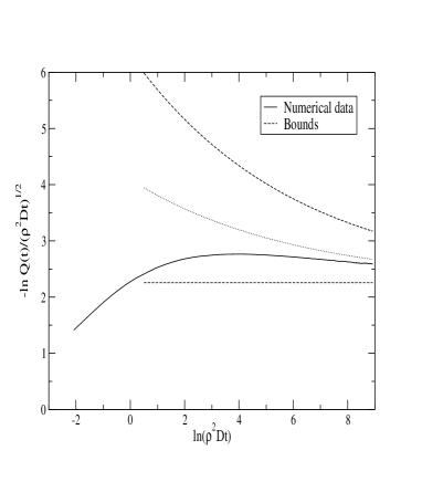
Figure 1: Bounds on the quantity $-\ln Q(t)/(\rho^{2}Dt)^{1/2}$. Continuous line: numerical data from ref.BB2 , with $\rho=1/2$ and $D=D_{A}=D_{B}=1/2$; dashed lines: rigorous upper and lower bounds; dotted line: new lower bound on $Q(t)$ valid for $D_{A}\ll D_{B}$.

In the following subsection we provide a finite-size scaling analysis which strongly suggests that the lower bound, $\hat{Q}_{1l}(t)$, gives the correct asymptotic form, $\hat{Q}_{1}(t)\sim\exp(-ct^{1/3})$, although the constant $c$ may differ from (i.e. be smaller than) that appearing in Eq. (35).

IV.4 Exact Diagonalization for finite $N$

One can show that the matrix elements $A_{mn}$ decay as a power law along the rows, so it is not obvious whether or not the off-diagonal matrix elements make a significant contribution to the eigenvalues. These off-diagonal terms do not enter the calculation of the lower bound $\hat{Q}_{1l}$, so it is clearly of interest to know whether they qualitatively change the result.

As an analytical insight is missing so far, we study this problem numerically using the eigenvalues of finite matrices $A^{N}_{mn}$ to compute $\hat{Q}_{1}(g,N)$ of Eq. (26). The latter equation gives

$$\hat{Q}_{1} = [\det(I+gA)]^{-1/2}$$ (36)

$$= \exp\left(-\frac{1}{2}\sum_{n=0}^{\infty}\ln(1+g\lambda_{n})\right)\ ,$$

where $I$ is the unit matrix and $\lambda_{n}$ is the $n$th eigenvalue of $A$ (where the eigenvalues are listed in decreasing order). Ideally, in a finite-$N$ analysis we would simply truncate the sum at $n=N$. In practice, of course, we do not know the eigenvalues explicitly, so instead we truncate the matrix $A$ to an $N\times N$ matrix and compute the eigenvalues of the truncated matrix.

In the asymptotic regime we anticipate the finite-size scaling form

$$-\ln[\hat{Q}_{1}(g,N)]=N^{\alpha}f(g/N^{\beta})\ .$$ (37)

The condition that $\hat{Q}_{1}(g,N)$ has an $N$-independent large-$N$ limit implies that $f(x)\sim x^{\alpha/\beta}$ for $x\rightarrow 0$.

It is instructive to first consider the diagonal approximation to the matrix $A$, in which the off-diagonal terms are neglected. This provides the lower bound $\hat{Q}_{1l}$ given by Eq.  (32). The corresponding finite-size quantity, $\hat{Q}_{1l}(g,N)$ is given by $\hat{Q}_{1l}(g,N)=\exp[-(1/2)\sum_{n=1}^{N}\ln(1+gA_{nn})$, leading to

$$-\ln[\hat{Q}_{1l}(g,N)]=\frac{1}{2}\sum_{n=1}^{N}\ln(1+gA_{nn})\ .$$ (38)

For large $n$, we show in the Appendix that $A_{nn}$ has the asymptotic form $A_{nn}\sim n^{-3/2}$, so the finite-size scaling variable is $g/N^{3/2}$, i.e.  $\beta=3/2$ in (37) within the diagonal approximation. In the limit $g\to\infty$, $N\to\infty$ with $g/N^{3/2}$ held fixed, one can replace the sum over $n$ by an integral and one readily recovers the scaling form (37) with $\alpha=1$, $\beta=3/2$. It is also easy to show that the scaling function $f(x)$ in Eq.  (37) has, within the diagonal approximation, the limiting forms $f(x)\sim x^{2/3}$ for $x\ll 1$, as expected, while $f(x)\sim\ln(x)$ for $x\gg 1$.

Our aim is to investigate whether the same general scaling structure (37), with the same exponents $\alpha=1$ and $\beta=3/2$, holds when the full matrix $A$ is used instead of just its diagonal part. If the matrix $A$ is simply truncated to an $N\times N$ matrix, however, and the eigenvalues determined, the corrections to finite-size scaling are found to be large. We attribute this to a large influence of the missing matrix elements $A_{mn}$, with $m$ or $n$ greater than $N$, on the eigenvalues $\lambda_{n}$ when $n$ gets close to $N$. Instead, therefore, we adopt a more refined approach in which the matrix is truncated to size $2N$, but we use only the first $N$ eigenvalues to compute $\hat{Q}_{1}(g,N)$. Furthermore, instead of computing $-\ln\hat{Q}_{1}(g,N)=(1/2)\sum_{n=1}^{N}\ln(1+g\lambda_{n})$, we compute the derivative

$$H(g,N) = -2\frac{d}{dg}\ln\hat{Q}_{1}(g,N)$$ (39)

$$= \sum_{n=1}^{N}\lambda_{n}/(1+g\lambda_{n})\ ,$$

since we find that corrections to finite-$N$ scaling are smaller for this quantity.

The finite-size scaling form for $H(g,N)$ follows from its definition and Eq. (37):

$$H(g,N)=N^{\alpha-\beta}h(g/N^{\beta})\ ,$$ (40)

where $h(x)=2\,df/dx$. On the basis of the diagonal approximation we expect $\alpha=1$, $\beta=3/2$, and $h(x)\to(4A/3)x^{-1/3}$ for $x\ll 1$, where $A$ is given by Eq. (34), and, from Eq. (39), $h(x)\to x^{-1}$ for $x\gg 1$. We therefore plot $N^{1/2}H(g,N)$ against the scaling variable $x=g/N^{3/2}$.

Figure 2: Scaling plot for $H(g,N)=-2(d/dg)\ln[\hat{Q}_{1}(g,N)]$ ($N=50,100,200,400,800,1600$), with scaling variable $x=g/N^{3/2}$. Continuous curves – full matrix; broken curves – diagonal matrix. The straight lines are the asymptotes for large and small scaling variable – see text.

Fig.  2 shows that a good scaling collapse is obtained with $\alpha=1$ and $\beta=3/2$. This result implies that $-\ln\hat{Q}_{1}\propto g^{2/3}\propto t^{1/3}$, i.e. the nondiagonal elements of the matrix $A$ do not qualitatively change the scaling of the pre-asymptotic correction to the survival probability. The straight lines in the Figure are the asymptotes dicussed above, with slopes $-1/3$ and $-1$ for small and large scaling variable respectively. The main curve actually contains both the full matrix (continuous lines) and the diagonal approximation (symbols), which lie almost on top of each other.

A very small deviation from perfect scaling is evident in the data. In fact, a slightly better fit is obtained with $\beta=1.4$ instead of 1.5. However, the same numerical scaling analysis applied to the diagonal matrix, where $\alpha=1$ and $\beta=3/2$ are exact, also yields, for the range of $N$ and $g$ covered by Fig. (2), an apparent best fit with $\beta\approx 1.4$. We conclude that, for the full matrix, $\beta=3/2$ is consistent with the data within the numerical precision. We conclude, finally, that the form of the leading correction to asymptopia given by the lower bound (33) is correct. Even the amplitude seems to be given rather accurately by the lower bound.

V Beyond the quadratic action

In the previous sections we have used the functional $\mu_{1}[z]$ correct to first order in the ratio $D_{A}/D_{B}$ of the diffusion constant of the particle to that of the traps. To this leading order, the parameter which controls the asymptotic behaviour is $g\propto D_{A}/\sqrt{D_{B}}$. We obtained the following asymptotic lower bound for the survival probability, $Q(t)$, of the $A$-particle in $d=1$:

$$Q(t)\geq\exp[-\lambda_{1}t^{1/2}-Ag^{2/3}+\cdots]$$ (41)

where $g=(D_{A}/D_{B})\lambda_{1}t^{1/2}/\pi^{3}$ and $A$ is a constant. This suggests, as discussed in the preceding section, that at large $D_{A}/D_{B}$ the new lower bound can cross the lower bound deduced from an “excluded volume” kind of argument BB ; BB2 , given by Eq. (15).

To escape from this apparent contradiction, one has to consider higher-order (in $D_{A}/D_{B}$) terms in the action. To go to next order, we start from Eq. (13), and expand the right-hand side up to order $z^{4}$. After a tedious but straightforward calculation, we obtain a result for the term order $z^{4}$ in the form of a sum of (multiple) integrals. Inserting the Fourier expansion (25) and rescaling the expansion coefficients $a_{n}$ as before to make them dimensionless, we can cast the action in the dimensionless form

$$S=S_{0}+gS_{1}+g\frac{D_{A}}{D_{B}}S_{2}+O([D_{A}/D_{B}]^{2}),$$ (42)

where

$$S_{0} =\frac{1}{2}\sum_{n}a_{n}^{2}$$ (43)

$$S_{1} =\frac{1}{2}\sum_{m,n}A_{mn}a_{m}a_{n}$$ (44)

$$S_{2} =\frac{1}{4}\sum_{m,n,p,q}A_{mnpq}a_{m}a_{n}a_{p}a_{q}$$ (45)

and the vertices $A_{mn}$, $A_{mnpq}$ are pure numbers. Eq. (42) enables us to extend the calculation of $\hat{Q}_{1}(t)$, Eq.  (26), to one higher order in $D_{A}/D_{B}$ by replacing the exponential in Eq. (26) by $\exp(-S)$ with $S$ given by Eq. (42).

While we have not carried out this program explicitly, the structure of the expansion (42) shows that the quadratic approximation is valid for small $D_{A}/D_{B}$. What is the effect of the higher order terms? For the case $D_{B}=0$ (where the traps are immobile) the asymptotic behavior has, in $d=1$, the known functional form $\exp(-ct^{1/3})$, where $c\propto\rho D_{A}^{1/3}$. It is plausible to assume that higher-order corrections change the coefficient $c$ but leave the exponent unaltered. Then, if the above series in $D_{A}/D_{B}$ is convergent, we obtain the asymptotic behavior of $Q(t)$, including the leading pre-asymptotic correction, in the form

$$Q(t)\sim\exp\left[-\frac{4}{\sqrt{\pi}}(\rho^{2}D_{B}t)^{1/2}-(\rho^{2}D_{A}t)^{1/3}F\left(\frac{D_{A}}{D_{B}}\right)\right]\ .$$ (46)

The function $F(x)$ has the limiting behavior $F(x)\to A_{1}x^{1/3}$ for $x\to 0$, with $A_{1}\leq(32)^{1/3}/\sqrt{3}$ from the lower bound (35), while $F(x)\to A_{2}$ for $x\to\infty$, where $A_{2}=3/2^{2/3}$ to match the known asymptotic behavior with immobile traps – the so-called Donsker-Varadhan problem DV . This latter limit agrees with Eq.  (15) (where $\mu_{0}=0$ for immobile traps). The reason is simple. In $d=1$, only the two immobile traps immediately to the left and right respectively of the $A$ particle play any role. Let the distances of these traps from the $A$-particle be $x$ and $y$ at $t=0$. Then the particle survives as long as it stays within the box of size $(x+y)$ defined by these two traps, so its asymptotic survival probability, averaged over $x$ and $y$, is given by $Q(t)\sim\rho^{2}\int_{0}^{\infty}dx\int_{0}^{\infty}dy\exp[-\rho(x+y)-\pi^{2}D_{A}t/(x+y)^{2}]$. Evaluating the integral by steepest descents for $t\to\infty$ one recovers Eq. (15) (with $\mu_{0}=0$).

VI Summary and Conclusion

In this paper we have addressed the issue of the leading correction to asymptopia in the long-time dynamics of the trapping reaction, $A+B\to B$. The main results are a new rigorous lower bound, valid in the limit $D_{A}\ll D_{B}$, on the survival probability of the $A$-particle, and a numerical analysis, based on finite-size scaling, indicating that the new lower bound contains the correct analytic form for the correction to asymptopia, namely a $t^{1/3}$ correction to the leading $t^{1/2}$ term in the exponential. The new bound agrees well, at late times, with numerical data, as shown in Figure 1. We also presented a conjecture, Eq. (46), for the form of the correction to asymptopia for general $D_{A}/D_{B}$, incorporating both extreme limits, $D_{A}\ll D_{B}$ and $D_{A}\gg D_{B}$.

Open questions to be addressed in future work include the generalization of the work presented here to higher spatial dimensions. Another interesting question, addressed briefly in BMB , is the scaling with time of the fluctuations of surviving trajectories. These can be studied starting from Eq.  (LABEL:eq:mu1quadrat), using the same Fourier decomposition of the trajectory as employed in this work. One finds that the fluctuations are subdiffusive as suggested in BMB and observed in numerical simulations MG . Details of these calculations will be presented in a separate publication.

Appendix A Diagonal elements of the matrix $A$

The matrix element $A_{mn}$ is given by the double integral

$$I_{mn} = mnA_{mn}=\int_{0}^{1}\frac{dx}{\sqrt{1-x}}\int_{0}^{x}\frac{dy}{\sqrt{y}(x-y)^{3/2}}$$

$$\times(\sin(n\pi x)-\sin(n\pi y))(\sin(m\pi x)-\sin(m\pi y))$$

which by variable substitutions $z=x-y$, $s=y$ and standard manipulations of the trigonometric functions can be reduced to a sum of one-dimensional integrals

$$I_{mn} = 2\pi\cos\frac{\pi(m-n)}{2}\int_{0}^{1}dz\frac{1}{z^{3/2}}\sin\frac{n\pi z}{2}\sin\frac{m\pi z}{2}$$ (48)

$$\times J_{0}\left(\frac{\pi}{2}(m-n)(1-z)\right)$$

$$+2\pi\cos\frac{\pi(m+n)}{2}\int_{0}^{1}dz\frac{1}{z^{3/2}}\sin\frac{n\pi z}{2}\sin\frac{m\pi z}{2}$$

$$\times J_{0}\left(\frac{\pi}{2}(m+n)(1-z)\right),$$

where $J_{0}(z)$ is the Bessel function of the first kind. The fact that $I_{mn}=0$ if $m+n=2p+1$ can be obtained from the initial formula, Eq. (A), if one notices that the kernel is symmetric at reflection about the line $y=1-x$.

For the diagonal elements, $m=n$, the leading large-$n$ contribution comes from the first integral

$$2\pi\int_{0}^{1}dz\frac{1}{z^{3/2}}\sin^{2}\frac{n\pi z}{2} \approx 2\pi\sqrt{n}\int_{0}^{\infty}\frac{1}{z^{3/2}}\sin^{2}\frac{\pi z}{2}$$ (49)

$$= \sqrt{2}\pi^{2}n^{1/2}$$

correct to leading order for large $n$. It follows that

$$A_{nn}\to\sqrt{2}\pi^{2}n^{-3/2}$$ (50)

for $n\to\infty$.

The calculation of the asymptotic behaviour of $A_{mn}$ at large $n$ with $m$ fixed and large is more elaborate. Since it is not needed here, we will defer it to a future publication.

References

- (1) V. Mehra and P. Grassberger, Phys. Rev. E 65, 050101 (2002).
- (2) A. J. Bray and R. A. Blythe, Phys. Rev. Lett. 89, 150601 (2002).
- (3) R. A. Blythe and A. J. Bray, Phys. Rev. E 67, 041101 (2003).
- (4) A. J. Bray, S. N. Majumdar, and R. A. Blythe, Phys. Rev. E 67, 060102(R) (2003).
- (5) G. Oshanin, O. Benichou, M. Coppey, and M. Moreau, Phys. Rev. E 66, 060101(R) (2002).
- (6) M. Moreau, G. Oshanin, O. Benichou, and M. Coppey, Phys. Rev. E 67, 045104(R) (2003).
- (7) D. Toussaint and F. Wilczek, J. Chem. Phys. 78, 2642 (1983).
- (8) M. Bramson and J. L. Lebowitz, Phys. Rev. Lett. 61, 2397 (1988); J. Stat. Phys. 62, 297 (1991).
- (9) M. Tachiya, Radiat. Phys. Chem. 21, 167 (1983).
- (10) A. Blumen, G. Zumofen, and J. Klafter, Phys. Rev. B 30, 5379 (1984).
- (11) M. D. Donsker and S. R. S. Varadhan, Comm. Pure. Appl. Math. 28, 525 (1975); B. D. Hughes, Random Walks and Random Environments, vol. 1 (Oxford University Press, New York, 1995), and references therein.