Spin-triplet $s$-wave local pairing induced by Hund’s rule coupling

Abstract

We show within the dynamical mean field theory that local multiplet interactions such as Hund’s rule coupling produce local pairing superconductivity in the strongly correlated regime. Spin-triplet superconductivity driven by the Hund’s rule coupling emerges from the pairing mediated by local fluctuations in pair exchange. In contrast to the conventional spin-triplet theories, the local orbital degrees of freedom has the anti-symmetric part of the exchange symmetry, leaving the spatial part as fully gapped and symmetric $s$-wave.

I Introduction

For the last two decades, discovery of unconventional superconductors have fueled intensive research for novel pairing mechanisms. Of particular interest have been the cuprate damascelli and heavy-fermion steglich systems where the very existence of superconductivity is quite surprising due to the strong Coulomb repulsion within the framework of the conventional Eliashberg-Migdal theory schrieffer . Recently discovered class of superconductors close to the ferromagnetic phase such as Sr₂RuO₄ mckenzie , UGe₂ saxena demand better understanding between symmetry and superconductivity which goes beyond the $s$-wave BCS theory.

One of the most puzzling aspects of the superconductivity in the strongly correlated regime is the role of the repulsive Coulomb interaction. Common belief is that the pairing mechanism is driven or assisted by the Coulomb repulsion to an attractive interaction between electrons which results in spatial or temporal structures in the superconducting wavefunction to avoid direct Coulomb repulsion. Even some conventional $s$-wave phonon-mediated superconductors such as alkali-doped fullerenes have also shown extraordinarily high transition temperatures hebard despite the strong Coulomb repulsion near the Mott transition lof ; murphy .

Even before the onset of superconductivity, direct Coulomb interaction is heavily renormalized away by electrons moving in a correlated manner to form a narrow resonance near chemical potential. The superconductivity in such regime should be understood in terms of those correlated electronic basis, typically called quasi-particles (QP). The problem of mutual renormalization effects between electron-electron and electron-phonon (el-ph) has received a great deal of interest resulting in different interpretations, ranging from the conventional Coulomb pseudopotential schrieffer ; pseudoU , field-theoretic approaches tesanovic ; newns to numerical analysis freericks . Recently, it has been pointed out han_sc that the symmetry of the el-ph interaction critically influences the pairing interaction where the two interactions are so interwoven that the effective pairing interaction cannot be reduced into a form similar to the McMillan formula mcmillan .

We show here on the basis of generic hamiltonians that local orbital correlations are crucial for the superconductivity and, in particular, predict the Hund’s rule (HR) induced superconductivity. We discuss the local pairing as mediated by self-generated fluctuations within the on-site interactions and show that the Coulomb interaction and multiplet interaction work in fundamentally different way than described in perturbative theories. The HR superconductivity has the spin-triplet pairing state. In contrast to the well-known non-$s$-wave triplet pairing balian , the anti-symmetric part of the exchange symmetry of the pairing wavefunction is taken up by the local orbital variables, leaving the spatial part as the symmetric $s$-wave. We will discuss possible consequences of this new pairing structure.

This paper is organized as follows. In section II, we define the problem in models of multiplet interactions for Hund’s rule and Jahn-Teller el-ph couplings. In the following section III, the pairing mechanism is explained in a perturbation theory of a simplified dynamical mean field theory (DMFT). Results from full DMFT calculations are presented in the section IV and are discussed in detail. In Appendices Aand B, we describe the calculations for the local energy levels and perturbation theory. Finally, a new Hubbard-Stratonovich decoupling scheme for the Hund’s rule coupling which bypasses the sign-problem is introduced in Appendix C.

II models

We consider cases of doubly degenerate band electrons at half-filling which are locally coupled via Hund’s rule (HR) and Jahn-Teller (JT) phonons. We model the multi-band electronic system with the on-site Coulomb repulsion of strength $U$ as

$$H = -\sum_{ijm\sigma}t_{ij}d^{\dagger}_{im\sigma}d_{jm\sigma}-\mu\sum_{i}N_{i}$$ (1)

$$+{U\over 2}\sum_{i}N_{i}(N_{i}-1)+\sum_{i}H_{\rm mult}(i),$$

where $d^{\dagger}_{im\sigma}\,(d_{im\sigma})$ is the electron creation (annihilation) operator acting on site $i$, orbital $m\,(=1,2)$, spin $\sigma$, $\mu$ is the chemical potential and $N_{i}=\sum_{m\sigma}n_{im\sigma}$. The hopping integral $t_{ij}$ is chosen to give a semi-elliptical density of states with the half-bandwidth $W/2=1$ DMFT . The local multiplet interaction is taken as $H_{\rm mult}=H_{\rm HR}$ or $H_{\rm JT}$ han_sc ,

$$H_{\rm HR} = K\left[\sum_{m}n_{m\uparrow}n_{m\downarrow}\!-\!\!\!\sum_{m\neq m^{\prime}}\!\!n_{m\uparrow}n_{m^{\prime}\downarrow}\!-2\!\!\!\!\sum_{\sigma,m<m^{\prime}}\!\!\!\!n_{m\sigma}n_{m^{\prime}\sigma}\right]$$ (2)

$$+ K\!\!\sum_{m\neq m^{\prime}}\!\!\left(d^{\dagger}_{m\uparrow}d^{\dagger}_{m\downarrow}d_{m^{\prime}\downarrow}d_{m^{\prime}\uparrow}+d^{\dagger}_{m\uparrow}d^{\dagger}_{m^{\prime}\downarrow}d_{m\downarrow}d_{m^{\prime}\uparrow}\right),$$

$$H_{\rm JT} = {1\over 2}\sum_{\nu}\left(\dot{\varphi_{\nu}}^{2}+\omega_{\rm ph}^{2}\varphi_{\nu}^{2}\right)$$ (3)

$$+ \!\!\!{g\over\sqrt{\omega_{\rm ph}}}\!\sum_{\sigma}\!\!\left[\varphi_{1}(n_{1\sigma}-n_{2\sigma})+\varphi_{2}(d^{\dagger}_{1\sigma}d_{2\sigma}+{\rm h.c.})\right],$$

where the site index $i$ has been omitted for brevity. $K$ is the HR coupling constant and $\varphi_{\nu}$ $(\nu=1,2)$ are the phonon fields with the bare frequency $\omega_{\rm ph}$, and $g$ the el-ph coupling constant. In the anti-adiabatic limit of phonons ($\omega_{\rm ph}\rightarrow\infty$) tosatti , $H_{\rm JT}$ maps to the same form as $H_{\rm HR}$ but with a negative (fictitious) $K_{\rm JT}=-2\Delta$ ($\Delta\equiv g^{2}/\omega_{\rm ph}$). Therefore, the el-ph superconductivity is suppressed as the physical HR coupling is turned up. We will show that, as $K$ increases further, superconductivity re-emerges in a spin-triplet channel.

III Local pairing mechanism

We describe main ideas behind the local pairing before presenting results from the full dynamical mean field theory. In the strongly correlated regime, QP states within the energy band $[-zW,zW]$ ($z$ the QP renormalization factor, $W$ non-interacting bandwidth) are usually responsible for low-energy manybody phenomena. The effect of $U$ is implicit in the renormalization factor $z$ and the truncated high energy states. In such limit, we simplify the DMFT by singling out the QP band and ignore incoherent high energy excitations as

$$H_{\rm eff}=H_{\rm int}\!+\!\!\sum_{m{\bf k}\sigma}\!\!\left[\epsilon_{q{\bf k}}n_{m{\bf k}\sigma}\!+\!{t_{q}\over\sqrt{N_{s}}}(c^{\dagger}_{m{\bf k}\sigma}d_{m\sigma}\!+h.c.)\right],$$ (4)

where $c^{\dagger}_{m{\bf k}\sigma}\,(c_{m{\bf k}\sigma})$ is creation (annihilation) of a QP state, $\epsilon^{q}_{\bf k}$ is QP energy (absorbing chemical potential), $t_{q}\,(\sim zW)$ is hopping integral on and off the impurity and $N_{s}$ is the number of sites. Contributions from the high energy states are correctly considered in the full DMFT calculations. $H_{\rm int}$ is the interacting part of the original hamiltonian. Note that the interaction only acts on the impurity site. For small QP bandwidths with $zW$ smaller than other energy scales, we further simplify the above effective hamiltonian to a two-site model,

$$H_{\rm int}=H_{\rm mult}+\epsilon_{q}N_{c}+t_{q}\sum_{m\sigma}(c^{\dagger}_{m\sigma}d_{m\sigma}+h.c.),$$ (5)

with $c^{\dagger}_{m\sigma}=\sqrt{N_{s}^{-1}}\sum_{\bf k}c^{\dagger}_{m{\bf k}\sigma}$, $N_{c}=\sum_{m{\bf k}\sigma}n_{m{\bf k}\sigma}$ and $\epsilon_{q}$ the QP energy ($\epsilon_{q}\approx 0$), where the narrow QP band is represented by a single energy level. $H_{\rm eff}$ has the similar construction as the exact diagonalization implementation of the DMFT, where the bath spectrum is sampled with a finite number of energy levels DMFT . Representing the QP states with several discrete levels over a small energy range made little change. This procedure is expected to be valid as long as the electrons slow down by the strong Coulomb interaction so that the local picture is meaningful and there is a QP reservoir which supplies particles at an infinitesimal energy cost.

We solve the two-site problem Eq. (5) using the exact diagonalization method. We analyze the solution as a perturbation expansion in $t_{q}$ metzner . We estimate the pairing correlation by computing the energy gain $E_{p}$ for creating two extra electrons on a half-filled impurity site,

$$E_{p}=[E(N_{d}\!+\!2)-E(N_{d})]-2[E(N_{d}\!+\!1)-E(N_{d})],$$ (6)

where $E(n)$ is the ground state energy with $n$ total electrons and $N_{d}$ is the orbital degeneracy ($N_{d}=2$). It is crucial to have multiple electrons per site for the local multiplets to induce the local pairing. As shown in Ref. han_sc , the local pairing has a strong filling dependency.

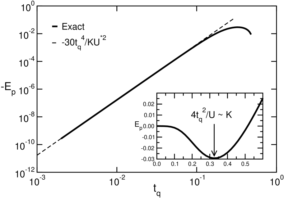
Figure 1: Pair correlation energy $E_{p}$ for two-site model Eq. (5) with the Hund’s rule coupling. $E_{p}$ is attractive for a wide range of hopping integral to the quasi-particle bath, $t_{q}$. Coupling to quasi-particle bath (thick line) produced a good agreement with the perturbation theory, $-30t_{q}^{4}/KU^{*2}$ ($U^{*}=U+2K$). The optimal interaction is at $4t_{q}^{2}/U\sim K$ for the maximum pair attraction $E_{p}\propto-K$.

Figure 2: Single site energy level scheme for two on-site electrons ($N_{d}=2$) with Hund’s rule and Jahn-Teller couplings. The degeneracy of 6 is lifted by the multiplet interaction $H_{\rm mult}$. The ground states are spin-triplet ($S=1$) and spin-singlet ($S=0$) for Hund’s rule. The Jahn-Teller multiplets have inverted level structure of the Hund’s rule coupling.

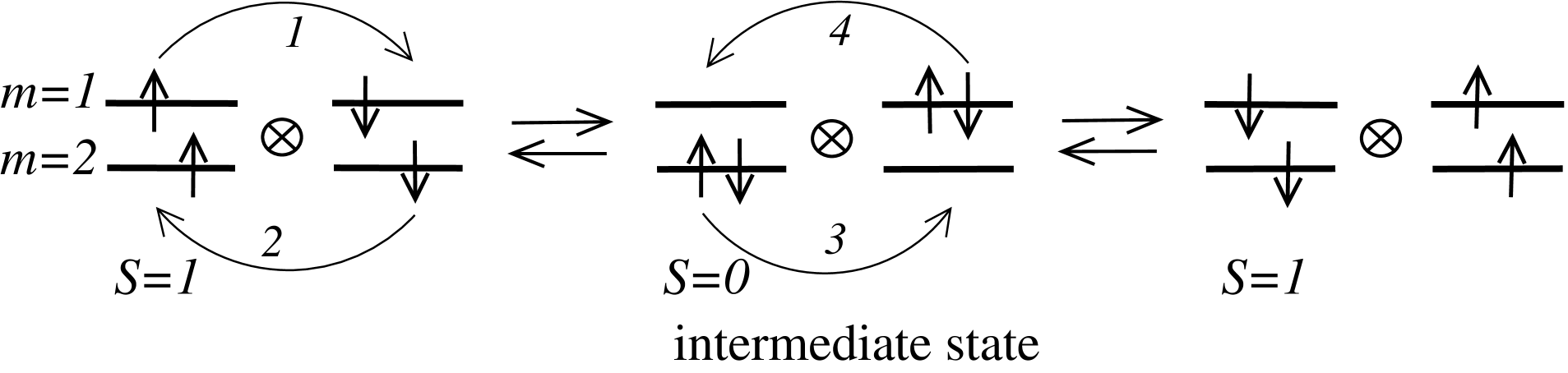
Figure 3: One of the contributions in $E(N_{d}+2)$ for the pair correlation energy $E_{p}$ in Eq. (20). Two extra electrons created on the interacting site dissolve into the quasi-particle bath to avoid Coulomb repulsion, which produces the ground state configurations shown on the left and right panel. The two unperturbed degenerate ground states couple via exchange of the spin-triplet electron pairs in the 4-th order perturbation of $t_{q}$ (from the left configuration to the right). In the intermediate state, the spins on the interacting site are in a locally excited state (See Fig. 2).

Numerical results shown for the HR problem are with parameters of $U=4$ and $K=0.1$. For small $t_{q}$ in a HR system, $E_{p}$ is negative (thick line in Fig. 1), i.e., it is energetically favorable to create mutually interacting quasi-particles than to create two independent quasi-particles. The impurity ground states are always predominantly of filling $N_{d}(=2)$ with the total spin $S=1$ since any extra electrons created on the impurity are repelled by the Coulomb interaction and are immediately dissolved into the QP bath. Therefore we first examine the atomic limit ($t_{q}=0$). Without $H_{\rm mult}$ the degeneracy of two-electron configurations is 6. The HR coupling lifts the degeneracy with the ground states of spin-triplet $(S=1)$ on the impurity site with

$$|T_{m})=\left\{d^{\dagger}_{1\uparrow}d^{\dagger}_{2\uparrow},{1\over\sqrt{2}}\left(d^{\dagger}_{1\uparrow}d^{\dagger}_{2\downarrow}-d^{\dagger}_{2\uparrow}d^{\dagger}_{1\downarrow}\right),d^{\dagger}_{1\downarrow}d^{\dagger}_{2\downarrow}\right\}|vac),$$ (7)

with $m=+1,0,-1$, respectively (see FIG. 2 and Appendix A). The 1st excitation energy is $2K$ for the HR coupling. The local energetics is described in Appendix A. Upon adding two electrons to the interacting site, the extra charges are immediately pushed to the QP reservoir to avoid the Coulomb repulsion. Through intersite hopping, the ground state triplet degeneracy is lifted. The resulting leading order ground state wavefunction has the most symmetric form ($U\gg K\gg t_{q}>0$),

$$|\psi_{0}^{N_{d}+2}\rangle={1\over\sqrt{3}}\left\{|T_{1})\otimes|t_{\bar{1}})+|T_{0})\otimes|t_{0})+|T_{\bar{1}})\otimes|t_{1})\right\},$$ (8)

where the second ket-vectors for the QP states in the direct products have similar definitions as Eq. (7). We analyze the perturbed ground state wavefunction and its energy in terms of the perturbation theory developed in Appendix B. The first order perturbed wavefunction becomes from Eq. (35),

$$|\psi_{1}^{N_{d}+2}\rangle = {\sqrt{3}t_{q}\over U^{*}}\left(d^{\dagger}_{1\uparrow}d^{\dagger}_{2\uparrow}d^{\dagger}_{1\downarrow}c^{\dagger}_{2\downarrow}-d^{\dagger}_{2\uparrow}c^{\dagger}_{1\uparrow}c^{\dagger}_{1\downarrow}c^{\dagger}_{2\downarrow}\right.$$

$$+ \left.d^{\dagger}_{1\uparrow}c^{\dagger}_{2\uparrow}d^{\dagger}_{1\downarrow}d^{\dagger}_{2\downarrow}-c^{\dagger}_{1\uparrow}c^{\dagger}_{2\uparrow}d^{\dagger}_{2\downarrow}c^{\dagger}_{1\downarrow}-(1\leftrightarrow 2)\right)|vac\rangle,$$

with the ionization energy $U^{*}/2=U/2+K$. This intermediate state has an ionized impurity at the excited energy $U^{*}$. With Eq. (37) and $E_{0}-H_{0}=-U^{*}/2$, one gets the second order contribution to the energy

$$E_{2}=\left({\sqrt{3}t_{q}\over U^{*}}\right)^{2}(-U^{*}/2)\cdot 8=-{12t_{q}^{2}\over U^{*}},$$ (10)

where the figure 8 is from the number of terms in Eq. (III). The second order correction to the wavefunction from Eq. (36) becomes

$$|\psi_{2}^{N_{d}+2}\rangle={2\sqrt{3}t_{q}^{2}\over KU^{*}}\left[|S_{a})\otimes|s_{a})+|S_{b})\otimes|s_{b})-{1\over 2}|S_{c})\otimes|s_{c})\right],$$ (11)

where $|S_{a}),\,|S_{b})$ and $|S_{c})$ are spin-singlet excited states on the interacting site as defined in Appendix A. The QP configurations $|s_{a}),\,|s_{b}),\,|s_{c})$ are defined with the same symmetry as the impurity states.

One of the processes in the second order contribution is depicted in Fig. 3. Typical (unperturbed) basis states in the ground state are spin-triplets as shown on the left and right side. The two states couple via the electron hopping where a second-order intermediate state is shown in the middle. After two hoppings (eg. the processes 1 and 2 from the left configuration), the resulting intermediate state becomes a charge-neutral spin-singlet ($S=0$), which correspond to the term $|S_{a})\otimes|s_{a})$ in Eq. (11) and a local transition between the multiplets in Fig. 2. Other charge-excited intermediate states have small contributions to the transition amplitude (of order $K/U$ smaller).

From Eq. (38), the forth order correction to the energy becomes

$$E_{4} = \left({2\sqrt{3}t_{q}^{2}\over KU^{*}}\right)^{2}\left[-2K-2K-4K\left({1\over 2}\right)^{2}\right]$$ (12)

$$-{12t_{q}^{2}\over U^{*}}8\left({\sqrt{3}t_{q}\over U^{*}}\right)^{2}\approx-{60\,t_{q}^{4}\over KU^{*2}},$$

for $K\ll U^{*}$. The ground state energy $E(N_{d}+2)$ becomes

$$E(N_{d}+2)=U-{12\,t_{q}^{2}\over U^{*}}-{60\,t_{q}^{4}\over KU^{*2}}.$$ (13)

The first term is the (unperturbed) atomic-limit. The last term contributes to the pairing interaction. The denominator in Eq. (13) comes from two ionized states (with charging energy $U^{*}$ after the hoppings 1 and 3 in Fig. 3 for example) and one HR-excited state (with excitation energy $\sim 2K$ after the hopping 2).

Ground state for one extra (spin-up) electron can be obtained similarly. For hopping integrals smaller than other energy scales, the interacting site is predominantly of filling 2 and of spin-triplet. Therefore the ground state consists of $|T_{0})\otimes|c_{m\uparrow})$ and $|T_{1})\otimes|c_{m^{\prime}\downarrow})$ ($|c_{m\sigma})\equiv c^{\dagger}_{m\sigma}|vac)$). Due to the hopping interaction, states of total spins $S_{z}=\pm 3/2$ do not appear in the ground state. An explicit calculation gives the unperturbed ground state,

$$|\psi_{0}^{N_{d}+1}\rangle={1\over\sqrt{3}}\left\{|T_{0})\otimes|c_{1\uparrow})+\sqrt{2}|T_{1})\otimes|c_{2\downarrow})\right\}.$$ (14)

The larger coefficient for $|T_{1})\otimes|c_{2\downarrow})$ reflects more paths for hopping transitions for this configuration. Similar calculations as those with $N_{d}+2$ electrons give

$$|\psi_{1}^{N_{d}+1}\rangle\!\! = \!\!{2t_{q}\over\sqrt{6}U^{*}}\left\{3d^{\dagger}_{1\uparrow}d^{\dagger}_{2\uparrow}d^{\dagger}_{2\downarrow}+3d^{\dagger}_{1\uparrow}c^{\dagger}_{2\uparrow}c^{\dagger}_{2\downarrow}\right.$$ (15)

$$\left.-2d^{\dagger}_{2\uparrow}c^{\dagger}_{1\uparrow}c^{\dagger}_{2\downarrow}-d^{\dagger}_{2\uparrow}c^{\dagger}_{2\uparrow}c^{\dagger}_{1\downarrow}+c^{\dagger}_{1\uparrow}c^{\dagger}_{2\uparrow}d^{\dagger}_{2\downarrow}\right\}|vac\rangle$$

$$|\psi_{2}^{N_{d}+1}\rangle\!\! = \!\!{\sqrt{3}t_{q}^{2}\over KU^{*}}\left[|S_{a})\otimes|c_{2\uparrow})+|S_{b})\otimes|c_{1\uparrow})-{|S_{c})\otimes|c_{1\uparrow})\over 2}\right]$$ (16)

$$E(N_{d}+1) = U-{8t_{q}^{2}\over U^{*}}-{15t_{q}^{4}\over KU^{*2}}.$$ (17)

The state without extra electrons results in no energy gain in the 4-th order,

$$|\psi^{N_{d}}\rangle = \left(1+{2t_{q}\over U^{*}}\sum_{n\sigma}c^{\dagger}_{n\sigma}d_{n\sigma}\right)|T_{m})\otimes|vac)$$ (18)

$$E(N_{d}) = U-{4t_{q}^{2}\over U^{*}}.$$ (19)

Finally, the pairing correlation Eq. (6) becomes

$$E_{p}=-30t_{q}^{4}/KU^{*2},$$ (20)

which is in excellent agreement with the exact diagonalization results in the $t_{q}\ll K$ limit. It is interesting to note that $E_{p}$ becomes smaller for stronger $K$ due to the higher multiplet excitation energy. The exact diagonalization results show maximum attractive pair correlation for $4t_{q}^{2}/U\sim K$, where the effective hopping exchange energy is comparable to the internal excitation energy. Upon substitution for $t_{q}$ in Eq. (20), this relation gives $E_{p}\propto-K$ at the optimal pairing.

One can also interpret the pairing as arising from pair exchange. In Fig. 3, the spin-up ($S_{z}=1$) pair on the interacting site hops out via processes 1 and 3, while the spin-down pair hops back in via 2 and 4. The charge neutral intermediate state forces the temporal overlap between the hoppings of the pairs, producing the attractive interaction when viewed as a second order perturbation in terms of the pair-basis. The same general reasoning should apply to other types of local interactions in the strong-$U$ limit.

One can carry out the same perturbation analysis for the Jahn-Teller interaction Eq. (3), where the pairing energy gain $E_{p}$ is always negative. $E_{p}=-7t_{q}^{4}/\Delta{U^{*}}^{2}$ for $U\gg\Delta\gg t_{q}$, which retains the similar form as Eq. (20) for the HR coupling. Leading order wavefunctions and their perturbed energies are written down in Appendix B. On the other hand, for a pure Hubbard model without the multiplet terms ($H_{\rm mult}=0$), $E_{p}=344t_{q}^{4}/U^{3}>0$ suggesting no superconductivity, which is also supported by full DMFT calculations DMFT . With $H_{\rm mult}=0$, the electrons only interact with charge fluctuations making the local internal fluctuations irrelevant. The above perturbation results are summarized in Table 1.

	$K=\Delta=0$	$K>0$	$\Delta>0$
$U=0$	0	-	$\,\,-2\Delta$
$t_{q}^{2}/U\ll\Delta,K$	$344t_{q}^{4}/U^{3}$	$\,\,-30t_{q}^{4}/KU^{2}$	$\,\,-7t_{q}^{4}/\Delta U^{2}$

Table 1: The pair correlation energy for an effective 2-site 2-band model with Hund’s rule ($K>0$) and the Jahn-Teller el-ph ($\Delta>0$) coupling. For large $U$, both of the couplings produce attractive pairing energy. ($\Delta=g^{2}/\omega_{\rm ph}$.)

As the pairing correlation energy Eq. (20) and Table 1 suggest, the Coulomb interaction and the multiplet interaction (including the JT el-ph interaction) cannot be separated into a form similar to $\lambda-\mu^{*}$ as in the McMillan formula mcmillan , where the Coulomb interaction represented as the Coulomb pseudopotential $\mu^{*}$ interact additively with the multiplet interaction (eg. el-ph coupling) represented by the mass-renormalization factor $\lambda$.

IV Pairing instability: DMFT results

Although the 2-site model is suggestive of the nature of the pairing, we show the existence of superconductivity from a lattice calculation. The lattice hamiltonian Eq. (1) is solved within the DMFT which approximates one-particle self-energies and vertex corrections as momentum-independent and maps a lattice model to an effective quantum impurity problem. We solve the impurity problem using quantum Monte Carlo (QMC) technique without making any physical approximations other than discretizing the imaginary time. It has been known that the QMC technique often suffers from the sign-problem signproblem . DMFT-impurity models with the Hubbard and electron-phonon couplings have been known not to cause any serious sign problem for most of the physical parameter space han_sc . However, inclusion of the Hund’s rule coupling terms in Eq. (2) produced severe sign-problems han_DMFT when each of the interaction terms are decoupled by the discrete Hubbard-Stratonovich transformation hirsch , despite that the decoupled HR terms resemble the Jahn-Teller coupling. To overcome such problem, a new scheme of mixing discrete hirsch and continuous bss Hubbard-Stratonovich transformations has been used. This removed the problem with the average signs larger than 0.9 for most of the runs. Details of the procedure is given in Appendix C. It is speculated that the simulation is more stabilized by the built-in symmetry of orbitals in the new transformation in contrast to the poorly preserved orbital symmetry in incomplete QMC samplings of the old scheme.

The superconducting instability is probed by computing uniform pair susceptibility $\chi$. $\chi$ for the spin-triplet channel can be expressed in a Bethe-Salpeter equation as

$$\chi = \chi_{0}+\chi_{0}\Gamma\chi_{0}+\chi_{0}\Gamma\chi_{0}\Gamma\chi_{0}+\cdots$$ (21)

$$= \sqrt{\chi_{0}}(I-\sqrt{\chi_{0}}\,\Gamma\sqrt{\chi_{0}})^{-1}\sqrt{\chi_{0}},$$

where we have used the symmetrized form scalapino . $\chi_{0}$ is the propagator of two electrons independently propagating with zero net momentum, and $\Gamma$ is the effective pairing interaction. (See Fig. 4.) Eq. (21) is a shorthand for matrices with indices over the Matsubara frequency $\omega_{n}$. For the static uniform susceptibility, we only need in-coming electrons of net zero momenta and net zero frequency, as in Fig. 4. Due to the momentum and frequency conservation at each internal vertices of Feynman diagrams, any internal pair of legs in the ladder diagrams in Fig. 4 also have net zero momenta and frequencies. The uniform (uncorrelated) 2-particle propagator $\chi_{0}$ can be computed with the 1-particle Green function as $\chi_{0}(\omega_{n})=\sum_{\bf k}G({\bf k},\omega_{n})G({\bf-k},-\omega_{n})$. The ${\bf k}$-summation is performed within $\chi_{0}$ due to the locality of the DMFT. $\Gamma$ is approximated by a local quantity $\Gamma^{\rm loc}$ obtained from a local relation similar to Eq. (21),

$$\Gamma^{\rm loc}=[\chi_{0}^{\rm loc}]^{-1}-[\chi^{\rm loc}]^{-1}.$$ (22)

$\chi_{0}^{\rm loc}$ is the local (uncorrelated) 2-particle propagator, $\chi_{0}^{\rm loc}(\omega_{n})=G^{\rm loc}(\omega_{n})G^{\rm loc}(-\omega_{n})$, and the local triplet pair susceptibility $\chi^{\rm loc}$ is directly computed from QMC as

$$\chi^{\rm loc}(\tau_{1},\tau_{2},\tau_{3},\tau_{4})=\!\langle T[d_{1\sigma}^{\dagger}(\tau_{1})d_{2\sigma}^{\dagger}(\tau_{2})d_{2\sigma}(\tau_{3})d_{1\sigma}(\tau_{4})]\rangle.$$ (23)

Corresponding definition of $\chi^{\rm loc}$ for the singlet channel can be found in Ref. han_sc . Since $\chi^{\rm loc}$ are directly obtained from the QMC measurements and $\chi_{0},\,\chi_{0}^{\rm loc}$ are easily computed from the 1-particle self-energy, we derive the effective interaction kernel $\Gamma\,(\equiv\Gamma^{\rm loc})$ and the uniform pair susceptibility $\chi$ from Eqs. (21,22).

The transition temperatures are determined by when the maximum eigenvalue of the superconducting kernel $\sqrt{\chi_{0}}\,\Gamma\sqrt{\chi_{0}}$ in Eq. (21) approaches 1. For such condition, the effective interaction must be attractive ($\Gamma>0$). The other requirement is the finite weight of quasi-particles at the chemical potential as in $\chi_{0}(\omega)\approx\pi zN(0)/\omega$, with $N(0)$ non-interacting density of states at the chemical potential. As the system becomes strongly correlated, $\chi_{0}$ becomes smaller as $z\rightarrow 0$ while the effective local correlation tends to get larger as electrons are more localized. The resulting $T_{c}$ is determined by the balance between $\chi_{0}$ and $\Gamma$.

The attractive interaction $V_{\rm eff}(\omega_{n},\omega_{m})\,(\equiv-(1/T)\Gamma(\omega_{n},\omega_{m}))$ is shown in Fig. 5 for $U/W=0.6$ and $K/W=0.1$. It is quite interesting that $V_{\rm eff}(\omega_{n},\omega_{m})$ resembles that for the electron-phonon coupling in the Eliashberg theory schrieffer where $V_{\rm eff}(\omega_{n},\omega_{m})=g^{2}D(\omega_{n}-\omega_{m})$ with the phonon propagator $D(\omega_{n})$. The attractive part is formed in a uniform attractive valley along the small energy transfer region $\omega_{n}\approx\omega_{m}$. For pure Hubbard interactions, the effective interaction $V_{\rm eff}(\omega_{n},\omega_{m})$ shows a very different profile with high energy structures jarrell away from the low energy scattering $\omega_{n}=\omega_{m}$. The attractive interaction along the $\omega_{n}=\omega_{m}$ line clearly demonstrates that the HR-induced local pairing is mediated by the effective low-energy coupling medium which has been self-generated by the multiplet interaction. Since the local spin excitation energy is $2K$ (see Fig. 2) and the electron-spin coupling constant is of order $K$, a naive estimate for the effective interaction gives $\sim K^{2}(2/2K)\sim K(=0.2)$, as in the electron-phonon theory. The numerically obtained $V_{\rm eff}$ at $2-4$ is about an order of magnitude larger than the simple estimate. This suggests that the renormalization effect is very strong and is consistent with the above observation that the suppressed hopping due to the Coulomb interaction enhances the local interaction veff . A thorough examination of the renormalization effects is necessary to fully understand these numerical results. Diagrammatic methods will prove particularly useful when backed up by the QMC and the exact diagonalization methods since the basic mechanism of the local pairing is given as in Section III.

Figure 4: Expansion of spin-triplet pairing susceptibility $\chi$. The local index $m\sigma$ ($m=1,2$) is for orbital and spin labels.

Figure 5: The effective interaction $V_{\rm eff}(\omega_{n},\omega_{m})\,(\equiv-\Gamma(\omega_{n},\omega_{m})/T)$. The attractive interaction is for small energy transfer ($\omega_{n}\approx\omega_{m}$). The interaction at higher frequencies is repulsive.

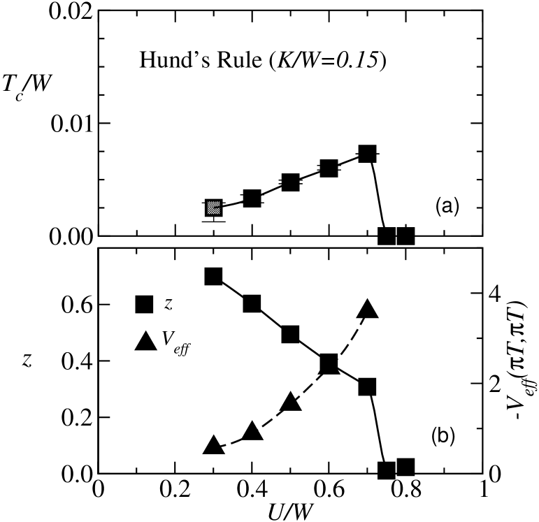
Figure 6: (a) Superconducting transition temperature $T_{c}$ vs Coulomb repulsion $U$ with Hund’s rule coupling. For the Hund’s rule (HR) coupled system, $T_{c}$ monotonically increases with $U$ showing local pairing mechanism. Gray symbol is an extrapolated estimate from the superconducting kernel $\chi_{0}\Gamma$. (b) Quasi-particle renormalization factor $z$ (left axis) and effective pairing interaction $V_{\rm eff}$ at lowest Matsubara frequency(right axis). $z$ decreases as $U$ approaches $U_{c}$. The product $zV_{\rm eff}$ for the HR system increased as $U\rightarrow U_{c}$, consistent with the increasing $T_{c}$. $W$ is the non-interacting bandwidth.

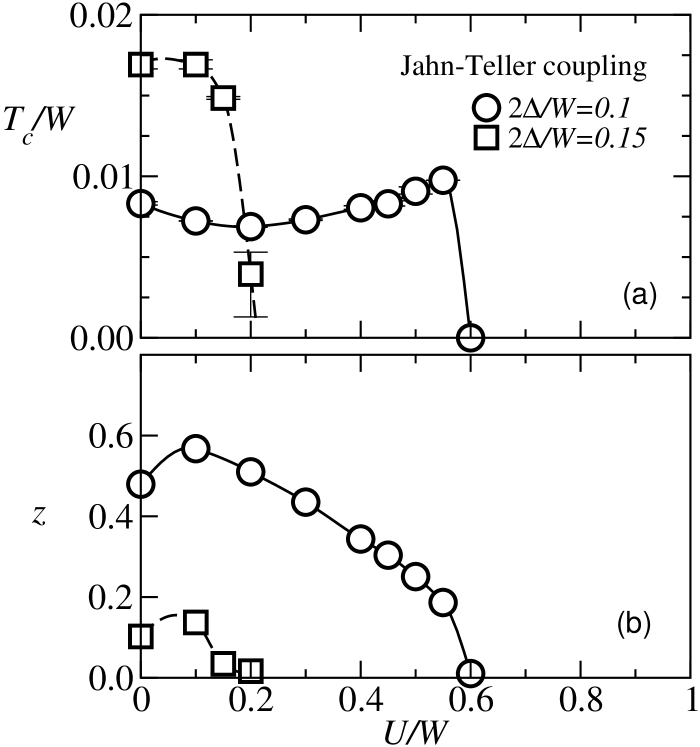
Figure 7: (a) Superconducting transition temperature $T_{c}$ vs Coulomb repulsion $U$ with Jahn-Teller electron-phonon coupling. The Jahn-Teller (JT) phonon coupling produces superconductivity with a cross-over from the conventional superconductivity (small $U$) to the local pairing regime (large $U$) for $2\Delta/W=0.1$. For a larger electron-phonon coupling ($2\Delta/W=0.15$), the Mott insulator transition happened at smaller $U$. (b) Renormalization factor $z$ as in Fig. 6.

Fig. 6(a) shows transition temperatures $T_{c}$ for the HR coupling as a function of the Coulomb repulsion $U$ where the superconductivity becomes stronger with $U$. The HR superconductivity emerged only in the spin-triplet channel. $T_{c}$ monotonically increased as $U$ approached the critical value $U_{c}/W\approx 0.75$ for $K/W=0.15$, a strong indication of the local pairing. $T_{c}/W$ less than 0.002 (gray symbol) has been estimated by extrapolating eigenvalues of the superconducting kernel $\sqrt{\chi_{0}}\Gamma\sqrt{\chi_{0}}$. The HR-coupled superconductivity is strong only in the local pairing regime, since at small $U$ there exists no external low-energy pairing medium in the electronic HR coupling.

$V_{\rm eff}(\pi T,\pi T)$ at the lowest Matsubara frequency at $T/W=1/120$ (triangles in Fig. 6(b), to the right-hand-side scale) show a growing local pairing attraction as $z\rightarrow 0$ veff . The product $zV_{\rm eff}(\pi T,\pi T)\,(\propto\chi_{0}\Gamma)$ increases as $U\rightarrow U_{c}$, consistent with the increasing $T_{c}$. We emphasize that the local pairing becomes apparent even at moderately correlated regime of $z\sim 0.5$, although the heuristic argument in section III was given for $z\rightarrow 0$ for the sake of clarity.

We can make some predictions based on general properties of the local spin-triplet pairing. (1) The exchange anti-symmetry is in the orbital space, in contrast to the $p$-wave spin-triplet theory balian . Due to the discreteness of orbitals, the quasi-particle excitation is gapped. The spatial part has the $s$-wave symmetry. (2) For large orbital degeneracy ($N_{d}>2$), coupling between different pairs of orbital indices will likely result in multiple gaps. (3) The local pairing is strong for high electron/hole dopings han_sc . For small dopings, ferromagnetic fluctuation will dominate the local triplet pairing. (4) As can be inferred from Fig 3, strong ferromagnetic order suppress the pair-exchange. Therefore, if the pairing and ferromagnetic phases ever co-exist, the superconducting phase should be near the ferromagnetic phase boundary.

Jahn-Teller phonon coupling (in Fig. 7) shows the similar behavior of the local pairing as the HR pairing. In contrast to the HR coupling case, $T_{c}$ is non-zero at $U=0$ with the pairing mediated by the external coupling medium of phonons. The results for $2\Delta/W=0.1$ shows that the phonon pairing-medium provides the attractive pairing for the small $U$ and as $U$ is increased further the superconductivity makes a cross-over to the local pairing regime. At large electron-phonon coupling ($2\Delta/W=0.15$) the metallic region shrunk and showed no signs of the cross-over. Given the same coupling strength (comparing $K$ and $|K_{\rm ph}|=2\Delta$), the HR system has weaker superconductivity than the el-ph systems.

One significant difference between this model of doubly degenerate orbitals (commonly called as $e\times E$ model) and the C₆₀ model ($t\times H$ model han_sc ) is that the $e\times E$ model produces stronger enhancement of $T_{c}$ in the local pairing regime. Authors in Ref. han_sc found no signs for the up-turn of $T_{c}$ near the Mott transition for any studied values of $\Delta$ in the C₆₀-model, although the enhancement of $T_{c}$ over the conventional theories was evident. It is probably due to the easier low spin formation for even fillings, since at odd number of fillings (as 3 in the C₆₀ model) unpaired spins tend to fluctuate via the intersite hopping and make the low spin configuration less effective.

Since the HR and JT couplings induce superconductivities separately but in different symmetries, they are expected to complete when both are present. For instance, by turning up the JT coupling constant at a fixed finite HR coupling, one can suppress the spin-triplet pairing and eventually crosses over to a spin-singlet pairing. It can be also anticipated from the mapping of the JT coupling to a negative HR hamiltonian in the anti-adiabatic limit. Fullerene systems are known to have sizable strengths for both interactions, although the JT interaction is more dominant for alkali-doped region. A recent density functional calculation study luders has suggested that the fullerene in the hole-doped region may have stronger Hund’s rule interaction, with possible applications to cation-doped fullerenes holedoped .

Finally, we make an observation of an interesting property of the local interaction Eq. (3). If we swap the spin and orbital indices in the JT coupling, Eq. (3), new boson fields $\tilde{\varphi}_{\nu}$ couple to electronic spin fluctuations, i.e., the coupling terms become $\sum_{m}[\tilde{\varphi}_{1}(n_{m\uparrow}-n_{m\downarrow})+\tilde{\varphi}_{2}(d^{\dagger}_{m\uparrow}d_{m\downarrow}+{\rm h.c.})]$. Now $\tilde{\varphi}_{\nu}$ plays the role of external local spin-fluctuations which mediate the electron pairing. All other terms in the hamiltonian are unchanged. The ground state now belongs in the spin-triplet and orbital-singlet space. The pair susceptibility for the singlet channel maps to that of the triplet-channel Eq. (23) and all results from JT coupling automatically hold for the triplet superconductivity. This model provides a robust example for the local spin-fluctuation superconductivity.

V Conclusion

We have demonstrated that the local pairing mechanism in multi-band systems on general grounds. In particular, the existence of Hund’s rule induced spin-triplet $s$-wave superconductivity is shown. The self-generated local multiplet fluctuations in the strong-$U$ limit provide the pairing medium even with a purely electronic interaction. This general idea should work for other extensions of the model. Further studies on the superconductor-ferromagnet phase diagram would clarify the relevance of the current model to known experimental systems. Fluctuation effects beyond the mean field approximation and singlet-triplet competition are left for future research.

Appendix A Atomic level scheme of Hund’s rule coupling

For 2 electrons on site, there are 6 possible configurations

$$\left\{d^{\dagger}_{1\uparrow}d^{\dagger}_{2\uparrow},\,d^{\dagger}_{1\downarrow}d^{\dagger}_{2\downarrow},\,d^{\dagger}_{1\uparrow}d^{\dagger}_{2\downarrow},d^{\dagger}_{2\uparrow}d^{\dagger}_{1\downarrow},d^{\dagger}_{1\uparrow}d^{\dagger}_{1\downarrow},d^{\dagger}_{2\uparrow}d^{\dagger}_{2\downarrow}\right\}|vac\rangle.$$ (24)

These states are degenerate for $H_{\rm mult}=0$. $H_{\rm mult}=H_{\rm HR}$ of Eq. (2) can be rewritten in the above basis set as

$$\left(\begin{array}[]{cccccc}-2K&0&0&0&0&0\\ 0&-2K&0&0&0&0\\ 0&0&-K&K&0&0\\ 0&0&K&-K&0&0\\ 0&0&0&0&K&K\\ 0&0&0&0&K&K\end{array}\right),$$ (25)

the solutions of which become

$$\begin{array}[]{ll}E=-2K,&\left\{\begin{array}[]{r}d^{\dagger}_{1\uparrow}d^{\dagger}_{2\uparrow}\\ 1/\sqrt{2}(d^{\dagger}_{1\uparrow}d^{\dagger}_{2\downarrow}-d^{\dagger}_{2\uparrow}d^{\dagger}_{1\downarrow})\\ d^{\dagger}_{1\downarrow}d^{\dagger}_{2\downarrow}\end{array}\right\}|vac\rangle\\ E=0,&\left\{\begin{array}[]{r}1/\sqrt{2}(d^{\dagger}_{1\uparrow}d^{\dagger}_{2\downarrow}+d^{\dagger}_{2\uparrow}d^{\dagger}_{1\downarrow})\\ 1/\sqrt{2}(d^{\dagger}_{1\uparrow}d^{\dagger}_{1\downarrow}-d^{\dagger}_{2\uparrow}d^{\dagger}_{2\downarrow})\end{array}\right\}|vac\rangle\\ E=2K,&1/\sqrt{2}(d^{\dagger}_{1\uparrow}d^{\dagger}_{1\downarrow}+d^{\dagger}_{2\uparrow}d^{\dagger}_{2\downarrow})|vac\rangle.\end{array}$$ (26)

As shown in Fig. 2, the ground states are $S=1$ spin-triplet and the excited states are $S=0$ spin-singlet with orbitally mixed states. The above ground multiplet states are written as $|T_{1}),\,|T_{0})$ and $|T_{\bar{1}})$ for the triplet states ($T$) of $S_{z}=1,0,-1$, respectively. Similarly, we write the above excited states as $|S_{a}),\,|S_{b})$ and $|S_{c})$, respectively, for spin-singlets ($S$). With one electron on site, the Hund’s rule coupling does not lift any degeneracy since it is a multi-electron interaction. The same is true with 3 electrons, since one can view this in terms of the hole interaction.

Appendix B Perturbation theory for pairing correlation energy

The perturbation is defined as an expansion with respect to the intersite hopping around the interacting Hamiltonian in Eq. (5),

$$H_{0} = UN(N-1)/2+H_{\rm mult}$$ (27)

$$V = -t_{q}\sum_{m\sigma}(c^{\dagger}_{m\sigma}d_{m\sigma}+h.c.).$$ (28)

First, let us develop a general perturbation theory up to the 4-th order. The Heisenberg equation reads

$$H|\psi\rangle=(H_{0}+V)|\psi\rangle=E|\psi\rangle,$$ (29)

where the energy eigenvalue and wavefunction are expanded in terms of the perturbation $V$ as

$$E = E_{0}+E_{1}+E_{2}+E_{3}+E_{4},$$ (30)

$$|\psi\rangle = |\psi_{0}\rangle+|\psi_{1}\rangle+|\psi_{2}\rangle+|\psi_{3}\rangle+|\psi_{4}\rangle.$$ (31)

The 0-th order terms give

$$H_{0}|\psi_{0}\rangle=E_{0}|\psi_{0}\rangle.$$ (32)

The $n$-st order equation becomes

$$H_{0}|\psi_{n}\rangle+V|\psi_{n-1}\rangle=\sum_{m=0}^{n}E_{m}|\psi_{n-m}\rangle.$$ (33)

Projecting the unperturbed bra-vector $\langle\psi_{0}|$ to Eq. (33) for $n=1$, one gets the first order correction to the energy

$$E_{1}=\langle\psi_{0}|V|\psi_{0}\rangle.$$ (34)

Introducing an operator $P_{0}$ which projects out the unperturbed wavefunction $|\psi_{0}\rangle$, one can express the wavefunction to the 1st order as,

$$|\psi_{1}\rangle={1\over E_{0}-H_{0}}P_{0}V|\psi_{0}\rangle.$$ (35)

The higher order contributions are computed by induction. The useful expressions up to the 4th order are

$$|\psi_{2}\rangle = {1\over E_{0}-H_{0}}P_{0}(V-E_{1})|\psi_{1}\rangle$$ (36)

$$E_{2} = \langle\psi_{0}|V|\psi_{1}\rangle=\langle\psi_{1}|(E_{0}-H_{0})|\psi_{1}\rangle$$ (37)

$$E_{4} = \langle\psi_{2}|(E_{0}-H_{0})|\psi_{2}\rangle-E_{2}\langle\psi_{1}|\psi_{1}\rangle,$$ (38)

where we have used a simplification $E_{1}=0$ which is the case with our models.

The unperturbed energies with the Jahn-Teller interaction, Eq. (3), at the total occupation numbers $N_{d},N_{d}+1,N_{d}+2$ are

$$E(N_{d}+2) = U-8\Delta-{4t_{q}^{2}\over U}-{14t_{q}^{4}\over\Delta U^{2}}$$ (39)

$$E(N_{d}+1) = U-8\Delta-{4t_{q}^{2}\over U}-{7t_{q}^{4}\over 2\Delta U^{2}}$$ (40)

$$E(N_{d}) = U-8\Delta-{4t_{q}^{2}\over U},$$ (41)

where $\Delta=-8g^{2}/\omega_{\rm ph}$ is the local Jahn-Teller coupling energy. Corresponding wavefunctions of the leading order are

$$|\psi(N_{d}+2)\rangle = |S_{c})\otimes|s_{c})$$ (42)

$$|\psi(N_{d}+1)\rangle = |S_{c})\otimes c^{\dagger}_{m\sigma}|vac)$$ (43)

$$|\psi(N_{d})\rangle = |S_{c})\otimes|vac),$$ (44)

with notations given in Appendix A.

Appendix C Hubbard-Stratonovich decoupling for Hund’s rule coupling

The discrete Hubbard-Stratonovich transformation hirsch (DHST) is given by

$$e^{-\Delta\tau Un_{\alpha}n_{\beta}}=e^{-{\Delta\tau U\over 2}(n_{\alpha}+n_{\beta})}{1\over 2}\sum_{\sigma}e^{\lambda\sigma(n_{\alpha}-n_{\beta})},$$ (45)

for fermion number operator $n_{\alpha}$ for a quantum state $\alpha$ and $\cosh\lambda=\exp(\Delta\tau U/2)$. The continuous Hubbard-Stratonovich transformation bss (CHST) applies to a general operator $\hat{A}$ in a gaussian integral

$$e^{\hat{A}^{2}}=\int dx\,\exp(-\pi x^{2}+\sqrt{\pi}\hat{A}x).$$ (46)

For doubly degenerate orbital systems, the interacting Hamiltonian Eq. (2) can be rewritten as

$$H_{\rm int} = {U\over 2}\left[N_{+}+N_{-}\right]^{2}$$

$$+ K\left[\sum_{m}n_{m\uparrow}n_{m\downarrow}\!-\!\!\!\sum_{m\neq m^{\prime}}\!\!n_{m\uparrow}n_{m^{\prime}\downarrow}\!-2\!\!\!\!\sum_{\sigma,m<m^{\prime}}\!\!\!\!n_{m\sigma}n_{m^{\prime}\sigma}\right]$$

$$+ K\!\!\sum_{m\neq m^{\prime}}\!\!\left[d^{\dagger}_{m\uparrow}d^{\dagger}_{m\downarrow}d_{m^{\prime}\downarrow}d_{m^{\prime}\uparrow}+d^{\dagger}_{m\uparrow}d^{\dagger}_{m^{\prime}\downarrow}d_{m\downarrow}d_{m^{\prime}\uparrow}\right],$$

where $N_{+}=\sum_{m}n_{m\uparrow}$ and $N_{-}=\sum_{m}n_{m\downarrow}$. Previously, each terms in the first two lines have been decoupled by the DHST. $N_{+}^{2},N_{-}^{2},N_{+}N_{-}$ are expanded into $n_{m\sigma}n_{m^{\prime}\sigma^{\prime}}$ terms before the DHST Eq. (45) is applied. The terms on the third line have been decoupled by

$$e^{-\Delta\tau Kc^{\dagger}_{\alpha}c^{\dagger}_{\beta}c_{\delta}c_{\gamma}}={1\over 2}\sum_{\sigma}e^{\sqrt{\Delta\tau K}\sigma(c^{\dagger}_{\alpha}c_{\gamma}-c^{\dagger}_{\beta}c_{\delta})},$$ (48)

where $K>0$ and no pairs of the indices from $\{\alpha,\beta,\gamma,\delta\}$ are the same. When the QMC sampling is incomplete, all the symmetry inherent in the original hamiltonian is not fully recovered, which is speculated to be a source of the sign-problem. This problem can be resolved by a different decoupling scheme as follows. We rewrite the first line as

$${U\over 2}(N_{+}+N_{-})^{2}=U(N_{+}^{2}+N_{-}^{2})-{U\over 2}S_{z}^{2},$$ (49)

with $S_{z}=N_{+}-N_{-}$. For the orbital degeneracy $N_{d}=2$, the first two terms in the second line in Eq. (C) can be written as

$$K\left(n_{1\uparrow}n_{1\downarrow}+n_{2\uparrow}n_{2\downarrow}-n_{1\uparrow}n_{2\downarrow}-n_{2\uparrow}n_{1\downarrow}\right)$$ (50)

$$= -{K\over 2}\left(n_{1\uparrow}-n_{2\uparrow}-n_{1\downarrow}+n_{2\downarrow}\right)^{2}$$

$$+{K\over 2}(N_{+}+N_{-})-K(n_{1\uparrow}n_{2\uparrow}+n_{2\downarrow}n_{1\downarrow}),$$

where the first term with squared term is decoupled with the CHST of a single auxiliary field. This procedure preserves the symmetry between orbital 1 and 2. The third line in Eq. (C) has been the source of the sign-problem han_DMFT . We express this by completing square as

$$K(c^{\dagger}_{1\uparrow}c^{\dagger}_{1\downarrow}c_{2\downarrow}c_{2\uparrow}+c^{\dagger}_{2\uparrow}c^{\dagger}_{2\downarrow}c_{1\downarrow}c_{1\uparrow}+\cdots)$$ (51)

$$= -{K\over 2}(c^{\dagger}_{1\uparrow}c_{2\uparrow}+c^{\dagger}_{2\uparrow}c_{1\uparrow}-c^{\dagger}_{1\downarrow}c_{2\downarrow}-c^{\dagger}_{2\downarrow}c_{1\downarrow})^{2}$$

$$+{K\over 2}(N_{+}+N_{-})-K(n_{1\uparrow}n_{2\uparrow}+n_{2\downarrow}n_{1\downarrow}).$$

Similarly to Eq. (50), the squared term preserves the orbital symmetry with a negative coefficient ($K>0$). With $-2(n_{1\uparrow}n_{2\uparrow}+n_{2\downarrow}n_{1\downarrow})=-(N_{+}^{2}+N_{-}^{2})+(N_{+}+N_{-})$ and adding Eqs. (49-51), we finally have

$$H_{\rm int}\!\! =\!\! 3K(N_{+}+N_{-})+(U-2K)(N_{+}^{2}+N_{-}^{2})$$ (52)

$$-{U\over 2}S_{z}^{2}-{K\over 2}\left(n_{1\uparrow}-n_{2\uparrow}-n_{1\downarrow}+n_{2\downarrow}\right)^{2}$$

$$-{K\over 2}(c^{\dagger}_{1\uparrow}c_{2\uparrow}+c^{\dagger}_{2\uparrow}c_{1\uparrow}-c^{\dagger}_{1\downarrow}c_{2\downarrow}-c^{\dagger}_{2\downarrow}c_{1\downarrow})^{2},$$

where the $N_{\pm}$ in the first line are expanded into $n_{m\sigma}n_{m^{\prime}\sigma^{\prime}}$ and decoupled by the DHST, Eq. (45). Terms in the second and third lines are decoupled by the CHST, Eq. (46). With the old DHST scheme for all interaction terms, there are 6 auxiliary fields for $n_{\alpha}n_{\beta}$ pairs and 4 for $c^{\dagger}_{\alpha}c^{\dagger}_{\beta}c_{\gamma}c_{\delta}$ terms, 10 in total per each time slice. The improved scheme has 2 discrete fields for $n_{1\uparrow}n_{2\uparrow}$, $n_{1\downarrow}n_{2\downarrow}$ in $N_{\pm}^{2}$ and 3 continuous fields per time slice. This procedure can be extended to higher degeneracy $N>2$. Although the arrangement in Eq. (50) is special for $N_{d}=2$, they can be decoupled by the DHST without causing the sign-problem. Terms like in Eq. (51) are problematic for the sign-problems in the impurity problem. Eq. (51) can be readily extended to higher degeneracy and the above procedure will likely remove the sign-problem in the Hund’s rule coupling.

References

• (1) For a recent review, see A. Damascelli, Z. Hussain, and Z.-X. Shen, Rev. Mod. Phys. 75, 473 (2003).
• (2) F. Steglich et al., Phys. Rev. Lett. 43, 1892 (1979).
• (3) J. R. Schrieffer, Theory of superconductivity, Addison-Wesley Publishing Company, New York (1994).
• (4) A. P. McKenzie and Y. Maeno, Rev. Mod. Phys. 75, 657 (2003).
• (5) K. G. Saxena et al., Nature 406, 587 (2000).
• (6) A. F. Hebard et al., Nature 350, 600 (1991).
• (7) R. W. Lof et al., Phys. Rev. Lett. 68, 3924 (1992).
• (8) D.W. Murphy et al., J. Phys. Chem. Solids 53, 1321 (1992); R.F. Kiefl et al., Phys. Rev. Lett. 69, 2005 (1992).
• (9) P. Morel and P. W. Anderson, Phys. Rev. 125, 1263 (1962).
• (10) J. H. Kim and Z. TeΕ‘anoviΔ‡, Phys. Rev. Lett. 71, 4218 (1993).
• (11) D. M. Newns, H. R. Krishnamurthy, P. C. Pattnaik, C. C. Tsuei, and C. L. Kane, Phys. Rev. Lett. 69, 1264 (1992).
• (12) J. K. Freericks and M. Jarrell, Phys. Rev. Lett. 75, 2570 (1995).
• (13) J. E. Han, O. Gunnarsson, and V. H. Crespi, Phys. Rev. Lett. 90, 167006 (2003).
• (14) W. L. McMillan, Phys. Rev. 167, 331 (1968).
• (15) R. Balian and N. R. Werthamer, Phys. Rev. 131, 1553 (1963).
• (16) A. Georges et al., Rev. Mod. Phys. 68, 13 (1996).
• (17) M. Capone, M. Fabrizio, C. Castellani, and E. Tosatti, Science 296, 2364 (2002).
• (18) W. Metzner, Phys. Rev. B 43, 8549 (1991).
• (19) E. Y. Loh, Jr., J. E. Gubernatis, R. T. Scalettar, S. R. White, D. J. Scalapino, and R. L. Sugar, Phys. Rev B 41, 9301 (1990).
• (20) J. E. Han, M. Jarrell and D. L. Cox, Phys. Rev. B 58, R4199 (1998).
• (21) R. M. Fye and J. E. Hirsch, Phys. Rev. B 38, 433 (1988).
• (22) R. Blankenbecler, D. J. Scalapino, and R. L. Sugar, Phys. Rev. D 24, 2278 (1981).
• (23) C. Owen and D. J. Scalapino, Physica (Amsterdam) 55, 691 (1971).
• (24) M. Jarrell, private communication.
• (25) $V_{\rm eff}$ is the effective interaction in terms of non-interacting basis instead of between quasi-particles in $E_{p}$, Eq.Β (20).
• (26) M. LΓΌders, N. Manini, P. Gattari, and E. Tosatti, Eur. Phys. J. B 35 57 (2003).
• (27) W. R. Datars and P. K. Ummat, Solid State Commun. 94, 649 (1995); A. M. Panich, H.-M. Vieth, P. K. Ummat, and W. R. Datars, Physica B 327, 102 (2003).