Noise and Measurement Efficiency of a Partially Coherent Mesoscopic Detector

Abstract

We study the noise properties and efficiency of a mesoscopic resonant-level conductor which is used as a quantum detector, in the regime where transport through the level is only partially phase coherent. We contrast models in which detector incoherence arises from escape to a voltage probe, versus those in which it arises from a random time-dependent potential. Particular attention is paid to the back-action charge noise of the system. While the average detector current is similar in all models, we find that its noise properties and measurement efficiency are sensitive both to the degree of coherence and to the nature of the dephasing source. Detector incoherence prevents quantum limited detection, except in the non-generic case where the source of dephasing is not associated with extra unobserved information. This latter case can be realized in a version of the voltage probe model.

I Introduction

Motivated primarily by experiments involving solid-state qubit systems, attention has recently turned to examining the properties of mesoscopic conductors viewed as quantum detectors or amplifiers Gurvitz ; AleinerQPC ; Levinson ; Buks ; Stodolsky ; KorotkovQPC ; AverinRLM ; MakhlinRMP ; DevoretNature ; KorotkovSN ; Pilgram ; Me ; Averin ; ShnirmanSmallV . Of particular interest is the issue of quantum limited detection– does a particular detector have the minimum possible back-action noise allowed by quantum uncertainty relations? Reaching the quantum limit is crucial to the success of a number of potential experiments in quantum information physics, including the detection of coherent qubit oscillations in the noise of a detector KorotkovSN . The measurement efficiency of a number of specific mesoscopic detectors has been studied Gurvitz ; KorotkovQPC ; AverinRLM ; DevoretNature ; Pilgram , as have general conditions needed for quantum limited detection Averin ; Me . Recent studies of a broad class of phase coherent mesoscopic scattering detectors Pilgram ; Me have helped establish a general relation between back-action noise, the quantum limit and information. The back-action charge noise of these detectors was found to be a measure of the total accessible information generated by the detector’s interaction with a qubit, and the quantum limit condition to imply the lack of any “wasted” information in the detector not revealed at its output.

An important unanswered question regards the role of detector coherence– does a departure from perfectly coherent transport in the detector necessarily imply a deviation from the quantum limit? One might expect that dephasing will have a negative impact, as there will now be extraneous noise associated with the source of dephasing. However, if there were unused phase information in the coherent system, one might expect the addition of dephasing to bring the detector closer to the quantum limit, as this unused phase information will be eliminated. Addressing the influence of dephasing concretely requires an understanding of its effects on the noise properties of a detector. In the case where the detector is a mesoscopic conductor, the influence of dephasing on the output current noise has received considerable attention Buttiker ; in contrast, its influence on the back-action charge noise has only been addressed in a limited number of cases ButtikerNote ; Seelig . Note that a recent experiment by Sprinzak et. alSprinzak using a point-contact detector suggests that the back-action noise is independent of dephasing.

To study the role of detector incoherence, we focus here on the case where the mesoscopic scattering detector is a non-interacting, single-level resonant tunneling structure, with the signal of interest (e.g., a qubit) modulating the energy of the level. This model provides an approximate description of transport through a quantum dot near a Coulomb blockade charge degeneracy point, in the limit where the dot has a large level spacing. Such a system could act as a quantum detector of, e.g., a double-dot qubit. The resonant level detector is also conceptually similar to detectors using the Josephson quasiparticle (JQP) resonance in a superconducting single electron transistor AverinJQP ; ChoiJQP ; ClerkJQP , as have been used in several recent qubit detection experiments NakamuraCPB ; KonradCPB . In these systems the resonance is between two transistor charge states, one of which is broadened by quasiparticle tunneling, and the signal of interest modulates the position of the resonance. Despite the incoherence of the resonance-broadening here, it has been shown theoretically that one can still make a near quantum-limited measurement using the JQP process ClerkJQP .

The detector properties of a fully coherent resonant level model were studied comprehensively by Averin in Ref. AverinRLM, , who found that detection can be quantum-limited in the small voltage regime (as follows also from the general analysis in Refs. Pilgram, and Me, ), and near-quantum limited in the large voltage regime. We are interested now in how the addition of dephasing changes these conclusions. The influence of dephasing on the noise properties of the resonant level model also has intrinsic interest, as this is one of the simplest systems with non-trivial energy-dependent scattering. Standard treatments ButtikerVProbe indicate that the effects of dephasing on the resonant level cannot be identified via the energy-dependence of the average current– both the coherent and incoherent models yield a Lorentzian form for the conductance. In contrast, the noise properties of the coherent and incoherent resonant level models are significantly different; while this is known for the current noise, we show that it can also hold for the back-action charge noise.

To study the effects of dephasing, we will use two general models. The first corresponds to dephasing due to unobserved escape from the level, and will be modelled using the voltage probe model developed by Büttiker ButtikerVProbe . The second will correspond to dephasing arising from a random time-dependent external potential. This approach is particularly appealing, as it allows a simple heuristic interpretation of the effects of dephasing, and allows for a clear separation between pure dephasing effects and inelastic scattering.

In general, we find that both the magnitude of dephasing and the nature of the dephasing source need to be determined in order to evaluate the effect of incoherence on the quantum limit. Dephasing prevents ideal quantum-limited detection, except in a simple, physically-realizable version of the voltage probe model. The latter model is unique, as one can show that there is no extra unobserved information produced by the addition of dephasing (i.e. the addition of the voltage probe). We also find that the voltage probe model can yield very similar noise properties to a sufficiently “slow” random potential model in the small voltage limit; this correspondence however is lost at larger voltages.

II Coherent Detector

We begin by briefly reviewing the properties of a coherent mesoscopic scattering detector, as discussed in Refs. Pilgram, and Me, . In the simplest case, the detector is a phase coherent scattering region coupled to two reservoirs ($1$ and $2$) via single channel leads, and is described by the scattering matrix:

$$s_{0}(\varepsilon)=e^{i\alpha_{0}(\varepsilon)}\left(\begin{array}[]{cc}e^{i\beta_{0}(\varepsilon)}\sqrt{1-T_{0}(\varepsilon)}&-i\sqrt{T_{0}(\varepsilon)}\\ -i\sqrt{T_{0}(\varepsilon)}&e^{-i\beta_{0}(\varepsilon)}\sqrt{1-T_{0}(\varepsilon)}\\ \end{array}\right).$$ (1)

There are three parameters which determine $s_{0}$: the overall scattering phase $\alpha_{0}(\varepsilon)$, the transmission coefficient $T_{0}(\varepsilon)$, and the relative phase between transmission and reflection, $\beta_{0}(\varepsilon)$. The only assumption in Eq. (1) is that time-reversal symmetry holds; as discussed in Ref. Me, , the presence or absence of time-reversal symmetry is irrelevant to reaching the quantum limit. Note that if $s_{0}$ has parity symmetry, the phase $\beta_{0}$ is forced to be zero, which implies that there is no energy-dependent phase difference between transmitted and reflected currents.

The conductor described by $s_{0}$ is sensitive to changes in the potential in the scattering region, and may thus serve as a detector of charge. A sufficiently slow input signal $v(t)$ which produces a weak potential in the scattering region will lead to a change in average current given by $\delta\langle I(t)\rangle=\lambda v(t)$, where $\lambda$ is the zero-frequency gain coefficient of the detector. In the case where the potential created by the signal (i.e. qubit) is smooth in the scattering region, and where the drain-source voltage tends to zero (i.e. $\mu_{1}=\mu_{2}+eV,eV\rightarrow 0$) the zero frequency noise correlators of the system are given by Pilgram ; Me :

$$\lambda = \frac{e^{3}V}{h}\partial_{\varepsilon}\big{|}[s_{0}(\varepsilon)]_{12}\big{|}^{2}=\frac{e^{3}V}{h}\partial_{\varepsilon}T_{0}(\varepsilon)$$ (2a)

$$S_{I} = \frac{2e^{3}V}{h}T_{0}(\varepsilon)R_{0}(\varepsilon)$$ (2b)

$$S_{Q} = \frac{e^{3}V\hbar}{\pi}\times$$ (2c)

$$\left(\frac{\left[\partial_{\varepsilon}T_{0}(\varepsilon)\right]^{2}}{4T_{0}(\varepsilon)R_{0}(\varepsilon)}+T_{0}(\varepsilon)R_{0}(\varepsilon)\left[\partial_{\varepsilon}\beta(\varepsilon)\right]^{2}\right)$$

Here, $S_{I}$ and $S_{Q}$ are the zero-frequency output current noise and back-action charge noise, $R_{0}\equiv 1-T_{0}$ is the reflection coefficient, and all functions should be evaluated at $\varepsilon=\mu$, where $\mu$ is the chemical potential of the leads. Note that the charge $Q$ here refers to the total charge in the scattering region, and is not simply the integral of the source-drain current $I$. Also note that throughout this paper, we concentrate on the case of zero temperature.

We are interested in the measurement efficiency ratio $\chi$, defined as

$$\chi\equiv\frac{\hbar^{2}\lambda^{2}}{S_{I}S_{Q}}.$$ (3)

In the case of a qubit coupled to the detector, $\chi$ represents the ratio of the measurement rate to the back-action dephasing rate in a quantum non-demolition setup MakhlinRMP ; DevoretNature ; Me , and the maximum signal to noise ratio in a noise-spectroscopy experiment KorotkovSN . $\chi$ is rigorously bounded by unity Averin ; Me , and reaching the quantum limit corresponds to having $\chi=1$. If we view our detector as a linear amplifier, achieving $\chi=1$ is equivalent to having the minimum possible detector noise energy Caves ; DevoretNature ; Me .

Even in the $V\rightarrow 0$ limit, the general 1D scattering detector described above fails to reach the quantum limit because of unused information available in the phase $\beta(\varepsilon)$:

$$\chi\equiv\frac{\hbar^{2}\lambda^{2}}{S_{I}S_{Q}}=\frac{1}{1+\left(2T_{0}R_{0}\frac{\partial_{\varepsilon}\beta_{0}}{\partial_{\varepsilon}T_{0}}\right)^{2}}$$ (4)

As noted, $\beta$ is the energy-dependent relative phase between reflection and transmission, and in principle is accessible in an experiment sensitive to interference between transmitted and reflected currents Sprinzak . The presence of parity symmetry would force $\beta=0$, and would thus allow an arbitrary one-channel phase-coherent scattering detector to reach the quantum limit in the zero-voltage limit KorotkovQPC ; Pilgram ; Me . Note that this discussion neglects screenings effects; such effects have been included within an RPA scheme in Ref. Pilgram, , where it was shown they did not effect $\chi$.

We now specialize to the case where our scattering region is a single resonant level. Taking the tunnel matrix elements to be independent of energy, the scattering matrix in the absence of dephasing is determined in the usual way by the retarded Green function of the level. Letting $1$ ($2$) denote the $L$ ($R$) lead, we have:

$$s_{0}(\varepsilon)=\hat{1}-i\sqrt{\Gamma_{i}\Gamma_{j}}\cdot G^{R}(\varepsilon)=\hat{1}-\frac{i\sqrt{\Gamma_{i}\Gamma_{j}}}{\varepsilon-\varepsilon_{d}+i\Gamma_{0}/2}$$ (5)

Here, $\Gamma_{L}$ ($\Gamma_{R}$) is the level broadening due to tunneling to the left (right) lead; $\Gamma_{0}=\Gamma_{L}+\Gamma_{R}$ represents the total width of the level due to tunneling. The parameters appearing in Eq. (1) are given by:

$$\alpha_{0}(\varepsilon) = -\arctan\left(\frac{\Gamma_{0}}{2(\varepsilon-\varepsilon_{d})}\right)$$ (6a)

$$T_{0}(\varepsilon) = \frac{\Gamma_{L}\Gamma_{R}}{(\varepsilon-\varepsilon_{d})^{2}+\Gamma_{0}^{2}/4}$$ (6b)

$$\beta_{0}(\varepsilon) = \arctan\left(\frac{\Gamma_{R}-\Gamma_{L}}{2(\varepsilon-\varepsilon_{d})}\right)$$ (6c)

Note that there is only one non-trivial eigenvalue of $s_{0}(\varepsilon)$, given by $e^{2i\alpha_{0}}$ (i.e. there is a scattering channel which decouples from the level).

One finds for the measurement efficiency at zero voltage:

$$\chi=\frac{(\varepsilon_{d}-\mu)^{2}}{(\varepsilon_{d}-\mu)^{2}+(\Gamma_{L}-\Gamma_{R})^{2}/4}$$ (7)

As per our general discussion above, the coherent resonant level detector is only quantum limited if there is parity symmetry, i.e. $\Gamma_{L}=\Gamma_{R}$; if this condition is not met, there is unused information available in the phase $\beta(\varepsilon)$. For the resonant level model, the effects of this unused information can be minimized by working far from resonance (i.e. $|\varepsilon_{d}-\mu|\gg 0$), as this suppresses the information in the phase $\beta(\varepsilon)$ faster than that in the amplitude $T_{0}(\varepsilon)$. It is worth noting that introducing a third lead to represent dephasing (as we do in the next section) breaks parity in a similar manner to simply having $\Gamma_{L}\neq\Gamma_{R}$, and its effect may be understood in similar terms. Note also that for $\Gamma_{L}=\Gamma_{R},\chi=1$ for any value of $\mu$. This may seem surprising as the gain vanishes when $\varepsilon_{d}=\mu$ (i.e. the peak of the resonance lineshape). However, the noise also vanishes at this point in just the manner required to maintain $\chi=1$. This feature does not carry over in any of the models of dephasing; $\chi$ will depend on the position of $\mu$ and will not be maximized for $\varepsilon_{d}=\mu$.

III Dephasing From Escape

III.1 General setup

We first treat the effects of dephasing by using the phenomenological voltage probe model developed by Buttiker ButtikerVProbe . A fictitious third lead is attached to the resonant level, with its reservoir chosen so that there is no net current flowing through it. Nonetheless, electrons may enter and leave this third lead incoherently, leading to a dephasing effect. We term this dephasing by escape, as it models electrons actually leaving the level. In practice, the Green function of the level is broadened by an additional amount $\Gamma_{\varphi}$ over the elastic broadening $\Gamma_{0}$; one also has to explicitly consider the contribution to the current and noise from electrons which enter and leave the voltage probe incoherently.

More concretely, assuming that there are $M$ propagating channels in the voltage probe lead, our detector is now described by a $(2+M)\times(2+M)$ scattering matrix $s_{big}$. We assume throughout the presence of time-reversal symmetry; the results presented here are independent of this assumption. The (non-unitary) $2\times 2$ sub-matrix of $s_{big}$ describing direct, coherent scattering between the physical leads is given by StoneLee :

$$\tilde{s}_{0}(\varepsilon)\equiv s_{0}(\varepsilon+i\Gamma_{\varphi}/2)$$ (8)

where $s_{0}(\varepsilon)$ is given by Eq. (5). This matrix continues to have a decoupled scattering channel (i.e. eigenvalue 1), while the eigenvalue of the coupled channel becomes:

$$e^{2i\alpha_{0}(\varepsilon)}\rightarrow\sqrt{1-T_{\varphi(\varepsilon)}}e^{2i\alpha(\varepsilon)}$$ (9)

with

$$\tilde{G}^{R}(\varepsilon) = \frac{1}{\varepsilon-\varepsilon_{d}+i\Gamma/2}$$ (10)

$$T_{\varphi}(\varepsilon) = \frac{\Gamma_{\varphi}\Gamma_{0}}{(\varepsilon-\varepsilon_{d})^{2}+(\Gamma/2)^{2}}$$ (11)

$$\alpha(\varepsilon) = \frac{1}{2}\left[\arg\tilde{G}^{R}(\varepsilon)-\arctan\left(\frac{\Gamma_{0}-\Gamma_{\varphi}}{2(\varepsilon-\varepsilon_{d})}\right)\right]$$ (12)

Here, $\Gamma=\Gamma_{0}+\Gamma_{\varphi}$ represents the total width of the level, $\tilde{G}^{R}(\varepsilon)$ is the retarded Green function of the level in the presence of dephasing, and $T_{\varphi}$ parameterizes the strength of the dephasing. Transmission into the voltage probe from the physical leads will be described by an $M\times 2$ sub-matrix of $s_{big}$ which we denote $t_{\varphi}$. Using a polar decomposition RMTReview , it may in general be written as:

$$\left[t_{\varphi}\right]_{mj}=\sum_{k=1,2}V_{mk}(\varepsilon)\sqrt{T_{\varphi,k}(\varepsilon)}U^{T}_{kj}(\varepsilon)$$ (13)

Here, $U$ and $V$ are unitary matrices which parameterize the preferred modes in the leads, and $T_{\varphi_{,}k}$ are the two transmission eigenvalues characterizing the strength of transmission into the voltage probe. These transmission eigenvalues are uniquely specified by $\tilde{s}_{0}(\varepsilon)$:

$$T_{\varphi,k}(\varepsilon) = \delta_{k1}T_{\varphi}(\varepsilon)$$ (14)

A general result of voltage probe models is that the average current $\langle I\rangle$ and current noise $S_{I}$ are independent of the matrices $U$ and $V$ appearing in the polar decomposition Buttiker ; deJong . This is convenient, because in general, these matrices are not uniquely determined by the form of the coherent scattering matrix $\tilde{s}_{0}(\varepsilon)$. However, in the present problem we are also interested back-action charge noise $S_{Q}$, which in general does depend on these matrices. For the dephased resonant-level, the matrix $U$ is completely specified by $\tilde{s}_{0}(\varepsilon)$:

$$U(\varepsilon)=e^{i\alpha(\varepsilon)/2}\left(\begin{array}[]{cc}e^{i\alpha(\varepsilon)/2}\cos\theta&-e^{-i\alpha(\varepsilon)/2}\sin\theta\\ e^{i\alpha(\varepsilon)/2}\sin\theta&e^{-i\alpha(\varepsilon)/2}\cos\theta\\ \end{array}\right)$$ (15)

where the angle $\theta=\tan^{-1}\sqrt{\Gamma_{L}/\Gamma_{R}}$ parameterizes the asymmetry in the coupling to the leads.

The matrix $V$ remains unknown; to specify it, we make the additional assumption that the voltage probe is coupled to the resonant level via a tunneling Hamiltonian with energy-independent tunnel matrix elements. This yields:

$$V_{m1}=-i\sqrt{\frac{\Gamma_{m}}{\Gamma_{\varphi}}}e^{-i\alpha(\varepsilon)}e^{i\arg\tilde{G}^{R}(\varepsilon)},$$ (16)

with $\Gamma_{\varphi}=\sum_{m=1}^{M}\Gamma_{m}$. Again, the ambiguity in $V(\varepsilon)$ has no affect on the average current through the system or on the current noise. It will however be important in determining the charge noise of the system; the choice given in Eq. (16) represents a best case scenario, in that it minimizes the charge noise.

Finally, we must specify the distribution function in the reservoir attached to the third lead. We will contrast three different choices which all yield a vanishing average current in the third lead, and which correspond to different physical mechanisms of dephasing Buttiker ; deJong . The first corresponds to a physically-realizable situation where the reservoir attached to the third lead has a well defined chemical potential; it is chosen to yield a vanishing average current into the probe. We term this the “pure escape” voltage probe model. The second model is similar, except one now also enforces the vanishing of the probe current at each instant of time by allowing the voltage associated with the third-lead to fluctuate BeenakkerButtiker . This model is usually taken to give a good description of inelastic effects, and is known as the inelastic voltage probe model. Finally, in the third model one also enforces current conservation as a function of energy. This is achieved by assigning a non-equilibrium distribution function to the reservoir deJong . This model is thought to well-describe quasi-elastic dephasing effects, and is known as the dephasing voltage probe model.

In what follows, we calculate the average current (and hence the gain $\lambda$), current noise $S_{I}$ and charge noise $S_{Q}$ from the scattering matrix $s_{big}$ describing the dephased resonant level detector. The standard relations between these quantities and the scattering matrix are given, e.g., in Ref. Me, . We will study the effects of dephasing by keeping the total width of the level $\Gamma$ constant, and varying its incoherent fraction $\Gamma_{\varphi}/\Gamma$. This is equivalent to asking how the noise and detector properties of a given Lorentzian conductance resonance of fixed width $\Gamma$ depends on the degree to which it is coherent. Of course, simply increasing dephasing while keeping the coupling to the leads fixed (e.g. by increasing temperature) would also cause the overall width $\Gamma$ to increase.

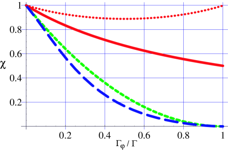
Figure 1: Quantum efficiency ratio $\chi$ versus $\Gamma_{\varphi}/\Gamma$ for the resonant level model, in the limit $eV/\Gamma\rightarrow 0$, and with symmetric couplings $\Gamma_{L}=\Gamma_{R}$. The solid red curve corresponds to the “pure escape” voltage probe model, the short-dashed green curve to the inelastic voltage probe model, and the long-dashed blue curve to the dephasing voltage probe model; each has $\varepsilon_{d}-\mu=\Gamma/2$. In addition, the dotted red curve corresponds to the “pure escape” model at $\varepsilon_{d}-\mu=10\Gamma$. For strong dephasing, only the “pure escape” model is able to remain near quantum-limited.

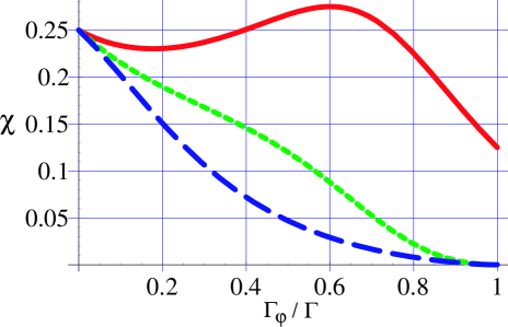
Figure 2: Quantum efficiency ratio $\chi$ versus $\Gamma_{\varphi}/\Gamma$ for the resonant level model, in the limit $eV/\Gamma\rightarrow 0$, and with $\Gamma_{L}\gg\Gamma_{R}$. We have chosen $\varepsilon_{d}=\Gamma/(2\sqrt{3})$ to maximize gain. The different curves correspond to different voltage probe models, as labelled in Fig. 1. Note the marked non-monotonic behaviour of $\chi$ in the “pure escape” voltage probe model.

III.2 Results from the “pure escape” voltage probe model

For simplicity, we focus throughout this subsection on the zero voltage limit. In general, the average current has both a coherent contribution (involving only the scattering matrix $\tilde{s}_{0}$) and an incoherent contribution, which involves transmission into the voltage probe lead Buttiker . These combine to yield the simple result ButtikerVProbe :

$$\langle I\rangle = \frac{e^{2}V}{h}\frac{2\Gamma_{L}\Gamma_{R}}{\Gamma_{L}+\Gamma_{R}}\left[-\textrm{Im }\tilde{G}^{R}(\varepsilon=\mu)\right]$$ (17)

$$= \frac{e^{2}V}{h}\left(\frac{\Gamma_{0}}{\Gamma}\right)\sin^{2}2\theta\frac{\Gamma^{2}/4}{(\mu-\varepsilon_{d})^{2}+\Gamma^{2}/4}$$

The conductance continues to have a Lorentzian form even in the presence of dephasing, though its overall weight is suppressed by a factor $(\Gamma_{0}/\Gamma)$; the gain $\lambda$ will be suppressed by the same factor. Note that this suppression is indistinguishable from simply enhancing the asymmetry between the couplings to the leads.

The effect of dephasing on the current noise is more pronounced. In the present model, even though the average current into the voltage probe vanishes, there may nonetheless exist fluctuating currents into and out of the voltage probe. The result is that measuring different linear combinations of the current in the left and right lead will yield different values for the current noise, though they all yield the same average current. Choosing the measured current to be the linear combination:

$$I_{meas}=(\sin^{2}\alpha)I_{L}+(\cos^{2}\alpha)I_{R},$$ (18)

and writing the current noise in terms of the Fano factor $f$:

$$S_{I}=2ef\langle I\rangle$$ (19)

one finds that in zero dephasing case, $f$ is independent of $\alpha$ and is given by the coherent reflection probability $(1-T_{0}(\varepsilon))$ (c.f. Eq. (6b)), whereas in the strong dephasing limit ($\Gamma_{0}/\Gamma\rightarrow 0$), it is given by:

$$f\rightarrow\sin^{4}\alpha+\cos^{4}\alpha$$ (20)

This form reflects the suppression of correlations between $I_{L}$ and $I_{R}$; $f$ ranges from a minimum of $1/2$ (for a symmetric combination of $I_{L}$ and $I_{R}$) to a maximum of $1$ if one measures either $I_{L}$ or $I_{R}$.

Turning to the charge noise, we find:

$$S_{Q}=\frac{e^{3}V\hbar}{2\pi}\left(\frac{2\Gamma_{L}\Gamma_{R}}{\Gamma_{0}^{2}}\right)\frac{\left[1-\left(\frac{\Gamma_{\varphi}}{\Gamma}\right)^{2}\right]\Gamma^{2}}{\left[(\mu-\varepsilon_{d})^{2}+\Gamma^{2}/4\right]^{2}}$$ (21)

Within the “pure escape” voltage probe model, $S_{Q}$ decreases monotonically with increasing dephasing, regardless of asymmetry or the position of the level. As was discussed in Ref. Me, , the charge noise $S_{Q}$ can be regarded as a measure of the total accessible information in a scattering detector. Thus, there is no “conservation of information” as dephasing is increased in the present model. In the strong dephasing limit, $S_{Q}$ is suppressed in the same way as $\langle I\rangle$ and $S_{I}$, that is by a factor $\Gamma_{0}/\Gamma$. We again emphasize that this result corresponds to a physically-realizable setup, where a third lead is attached to the level and assigned a well-defined chemical potential. The effect of a similar dephasor on the charge fluctuations of a quantum-point contact was studied experimentally by Sprinzak et. al in Ref. Sprinzak, ; in contrast to the result of Eq. (21) for the resonant level detector, they found that the addition of dephasing did not appreciably change the back-action noise of a quantum point-contact detector. Of course, the system studied in Ref. Sprinzak, is very different from the one studied here. Nonetheless, our result indicates that, at the very least, the insensitivity of charge fluctuations to dephasing seen in this experiment is not generic to all mesoscopic conductors.

Finally, turning to the measurement efficiency ratio $\chi$, we note that since each of $\lambda,S_{I}$ and $S_{Q}$ are suppressed as $\Gamma_{0}/\Gamma$, turning on dephasing does not lead to a parametric suppression of $\chi$ (see Figs. 1 and 2). In the strong dephasing limit, we find:

$$\chi\rightarrow\frac{1}{2f}\frac{(\mu-\varepsilon_{d})^{2}}{(\mu-\varepsilon_{d})^{2}+\Gamma^{2}/4},$$ (22)

where the Fano factor $f$ is given in Eq. (20). In the strong dephasing limit there is wasted phase information due to the strong asymmetry between the coupling to the physical leads and to the voltage probe lead. Nonetheless, the effects of this wasted phase information can be minimized by working far from resonance. Thus, for dephasing due to true escape (i.e. due to a simple third lead), one can approach the quantum limit even in the strongly incoherent limit. In this limit, all transport involves entering the voltage probe, and then leaving it incoherently. Nonetheless, in the small voltage limit we consider, there is no wasted amplitude information in the presence of dephasing. Though for energies in the interval $[\mu_{2},\mu_{3}]$ there is a current $I_{3,in}$ flowing into the voltage probe lead, one cannot learn anything new by measuring it, as an identical current exits the voltage probe in the energy interval $[\mu_{3},\mu_{1}]$ and contributes directly to the measured current flowing between the left and right contacts. It is this lack of wasted amplitude information that allows one to reach the quantum limit even for strong dephasing.

III.3 Results from the inelastic voltage probe model

As discussed earlier, the inelastic voltage probe model is identical to the “pure escape” model of the last subsection, except that we now also require that the current into the voltage probe vanishes at each instant of time. This is achieved on a semi-classical level by assigning the voltage probe a fluctuating-in-time voltage chosen to exactly enforce this additional constraintBeenakkerButtiker . The average current is independent of this additional step, and is identical to that in the previous section, Eq. (17). For the current noise, as we now have $I_{L}$ = $I_{R}$ at all times, $S_{I}$ becomes independent of the particular choice of measured current. In essence, the effect of the fluctuating voltage in the probe is to simply choose a particular value of $\alpha$ in Eq. (18) BeenakkerButtiker . In the strong dephasing limit, the Fano factor is given by:

$$f\rightarrow\frac{\Gamma_{L}^{2}+\Gamma_{R}^{2}}{(\Gamma_{L}+\Gamma_{R})^{2}}$$ (23)

Not surprisingly, this is the classical Fano factor corresponding to two Poisson processes in series. One also finds this Fano factor in the large voltage regime of the coherent resonant level model, where the model may be treated using classical rate equations DaviesRLM ; AverinOldRLM . Note that depending on the position of $\varepsilon_{d}$ and the ratio $\Gamma_{L}/\Gamma_{R}$, $f$ can either increase or decrease with increasing dephasing.

Finally, we turn to the calculation of the charge noise. The effects of the fluctuating voltage on $S_{Q}$ are far more extreme than on $S_{I}$ Thanks , as it leads to a new, classical source for charge fluctuations. Note that in general we have:

$$\langle Q\rangle=e\int d\varepsilon\rho(\varepsilon)\left(\frac{\Gamma_{L}f_{L}(\varepsilon)+\Gamma_{R}f_{R}(\varepsilon)+\Gamma_{\varphi}f_{3}(\varepsilon)}{\Gamma}\right)$$ (24)

where $\rho(\varepsilon)=\left(-\frac{1}{\pi}\textrm{Im}\tilde{G}^{R}(\varepsilon)\right)$. Fluctuations of the voltage in the probe lead will cause the probe distribution function $f_{3}(\varepsilon)$ to fluctuate, and will in turn cause $\langle Q\rangle$ to fluctuate. Letting $\Delta Q(t)$ denote the fluctuating part of the charge $Q$, one has Seelig :

$$\Delta Q(t)=\left[\Delta Q(t)\right]_{bare}+e\frac{\Gamma_{\varphi}}{\Gamma}\int d\varepsilon\rho(\varepsilon)\left(\Delta f_{3}(\varepsilon,t)\right)$$ (25)

The first term arises from fluctuations in the total current incident on the scattering region; it is the only contribution present in the absence of a fluctuating potential, and is identical to what is found in the “pure escape” model. The second term describes fluctuations of $\langle Q\rangle$ arising from voltage fluctuations in the voltage probe. These voltage fluctuations are in turn completely determined by the requirement that the current into the voltage probe vanish at all times BeenakkerButtiker . Note that as a result, the two terms in Eq. (25) will be correlated.

Including these effects, one finds that the charge fluctuations are given by:

$$S_{Q}=\left[S_{Q}\right]_{bare}+\left[S_{Q}\right]_{class}$$ (26)

Here, $[S_{Q}]_{bare}$ describes the intrinsic charge fluctuations (i.e. from the first term in Eq. (25)); its value is given by Eq. (21). The term $[S_{Q}]_{class}$ arises from fluctuations of $\Delta f_{3}$ (i.e. second term in Eq. (25)), and includes the effect of their correlation with $[\Delta Q]_{bare}$. It is given by:

$$\left[S_{Q}\right]_{class}=4e\hbar^{2}\frac{\Gamma_{\varphi}}{(\Gamma_{0})^{2}\Gamma}\left(1+\frac{\Gamma_{0}\Gamma_{\varphi}/2}{\omega^{2}+(\Gamma/2)^{2}}\right)|\langle I\rangle|$$ (27)

where $\langle I\rangle$ is given in Eq. (17), and where we have again taken the zero voltage limit. In the strong dephasing limit this contribution dominates, and we find:

$$S_{Q}\rightarrow 4e\hbar^{2}\frac{|\langle I\rangle|}{(\Gamma_{0})^{2}}$$ (28)

Unlike Eq. (21) for the intrinsic charge fluctuations, which are suppressed with increased dephasing, Eq. (27) describing the induced fluctuations of $Q$ diverges in the strong dephasing limit as $\Gamma/\Gamma_{0}$. As a result, the measurement efficiency $\chi$ tends to zero as $(\Gamma_{0}/\Gamma)^{2}$, and one is far from the quantum limit for strong dephasing. This result is not surprising. The fluctuating voltage in the probe lead represents a classical uncertainty in the system stemming from the source of dephasing; this uncertainty in turn leads to extraneous noise in $Q$, leading departure from the quantum limit. On a heuristic level, there is unused information residing in the voltage probe degrees of freedom responsible for generating the fluctuating potential. Of course, if this classical noise is ad-hoc suppressed, one is back at the “pure escape” model of the previous section, which can indeed reach the quantum limit even for strong dephasing.

III.4 Results from the dephasing voltage probe model

In the dephasing voltage probe model, the distribution function in the voltage probe reservoir is chosen so that the current flowing into the voltage probe vanishes at each energy Buttiker . One obtains a non-equilibrium distribution function $f_{3}(\varepsilon)$ defined by:

$$f_{3}(\varepsilon)=\bar{f}(\varepsilon)\equiv\frac{\Gamma_{L}f_{L}(\varepsilon)+\Gamma_{R}f_{R}(\varepsilon)}{\Gamma_{L}+\Gamma_{R}}$$ (29)

Similar to the inelastic voltage probe, we also enforce a vanishing current into the voltage probe at each instant of time by having $f_{3}(\varepsilon)$ fluctuate in time deJong . This model is usually thought to better mimic pure dephasing effects than the inelastic voltage probe, as the coupling to the voltage probe does not lead to a redistribution of energy.

For the average current in the small voltage regime, we again obtain Eq. (17), as in the “pure escape” model. In the finite voltage regime we obtain the simple result:

$$\langle I\rangle=\frac{e}{h}\frac{2\Gamma_{L}\Gamma_{R}}{\Gamma_{L}+\Gamma_{R}}\int d\varepsilon\left(f_{1}(\varepsilon)-f_{2}(\varepsilon)\right)\left(-\textrm{Im }\tilde{G}^{R}(\varepsilon)\right),$$ (30)

where again $\tilde{G}^{R}(\varepsilon)$ is the Green function of the level in the presence of dephasing (c.f. Eq. (10)). Eq. (30) is identical to the formally exact expression derived by Meir and Wingreen Meir for the current through a single level having arbitrary on-site interactions. Thus, we can think of the dephased Green function $\tilde{G}^{R}$ in the voltage probe approach as mimicking the effects of dephasing due to interactions. The simplicity of both the Meir-Wingreen and voltage-probe approaches (i.e. $\langle I\rangle\propto G^{R}$) may be simply extended to the multi-level case if the asymmetry in the tunnel couplings is the same for each level.

Turning to the noise, the main effect of the non-equilibrium distribution function $f_{3}$ will be to increase the noise over the previous two models. On the level of the calculation, these new contributions arise from diagonal elements of the current $I$ and charge $Q$ operators, considered in the basis of scattering states. More physically, this additional noise is due to the fact that the detector plus voltage probe system is no longer described by a single pure state. Rather, the distribution function $f_{3}$ corresponds to a statistical ensemble of states, with each state of the ensemble yielding a (possibly) different quantum expectation of $Q$ and $I$. The extra noise produced by this “classical” uncertainty corresponds to unused information (e.g. if the non-purity of the detector density matrix results from entanglement with a reservoir, the missing information resides in the reservoir degrees of freedom), and thus we anticipate a departure from the quantum limit even if we neglect the extraneous charge noise arising from the fluctuating voltage probe potential.

We find that the modification of the current noise is rather minimal– in the strong dephasing limit, one again obtains the classical Fano factor of Eq. (23). The effect on the charge noise is more pronounced. Similar to the inelastic voltage probe, there will be two contributions to $S_{Q}$, one stemming from fluctuations of the total incident current on the level, the other from fluctuations of the distribution function $f_{3}(\varepsilon)$. Separating the two contributions to $S_{Q}$ as in Eq. (26), we find for arbitrary voltages:

$$[S_{Q}]_{bare}=\frac{4e^{2}\hbar}{\pi}\int d\varepsilon\bar{f}(\varepsilon)\left(1-\bar{f}(\varepsilon)\right)\left(-\textrm{ Im }\widetilde{G}^{R}(\varepsilon)\right)^{2}$$ (31)

$$\left[S_{Q}\right]_{class}=\frac{4e^{2}\hbar}{\pi}\frac{\Gamma_{\varphi}}{\Gamma\Gamma_{0}}\int d\varepsilon\bar{f}(\varepsilon)\left(1-\bar{f}(\varepsilon)\right)$$

$$\left(-\textrm{ Im }\widetilde{G}^{R}(\varepsilon)\right)\left(1+\frac{2\Gamma_{0}\Gamma_{\varphi}}{\varepsilon^{2}+(\Gamma/2)^{2}}\right)$$ (32)

Interestingly, we find that in the dephasing voltage probe model, the intrinsic charge fluctuations $[S_{Q}]_{bare}$ (Eq. (31)) are independent of dephasing strength; the additional noise due to the non-equilibrium distribution function $\bar{f}$ exactly compensates the suppression of the intrinsic noise found in the “pure escape” model and inelastic voltage probe models (c.f. Eq. (21)). Recall that $S_{Q}=[S_{Q}]_{bare}$ in the absence of voltage fluctuations in the voltage probe lead.

The extrinsic contribution $[S_{Q}]_{class}$ (Eq. (32)) is similar in form to the corresponding contribution for the inelastic voltage probe model. In the strong dephasing limit this term dominates, and at arbitrary voltage, we again obtain the divergent result of Eq. (28) for $S_{Q}$. Similar to the inelastic voltage probe model, the fluctuations of $Q$ induced by the fluctuating probe voltage will cause a suppression of $\chi$ as $(\Gamma_{0}/\Gamma)^{2}$ in the strong dephasing limit. Note that even if one did not use a fluctuating voltage in the voltage probe (i.e. enforce current conservation in energy but not in time), and hence had only the intrinsic contribution to $S_{Q}$, one would still have a parametric suppresion of $\chi$ at strong dephasing; this is in contrast to the inelastic voltage probe model, where it is only $[S_{Q}]_{class}$ that prevents reaching the quantum limit at strong dephasing. Including all terms in $S_{Q}$, one finds that the meaurement efficiency for the dephasing voltage probe model is always less than that for the inelastic dephasing voltage probe model (see Figs. 1 and 2). As discussed above, these result follows from the additional classical uncertainty resulting from the voltage probe plus detector system being in a mixed state.

Finally, it is interesting to consider the case of a large voltage ($\mu_{L}-\mu_{R}=eV\gg\Gamma$) “co-tunneling” regime, where the level is placed slightly above the higher chemical potential $\mu_{L}$. Averin AverinRLM demonstrated that in the fully coherent case, one can still come close to the quantum limit (i.e. $\chi\rightarrow 3/4$) in this regime despite the loss of information associated with the large voltage and the consequent energy averaging. One might expect $\chi$ to be insensitive to dephasing in this regime, given the large voltage. This is not the case; as is shown in Fig. 3, $\chi$ is again suppressed to zero as $(\Gamma_{0}/\Gamma)^{2}$.

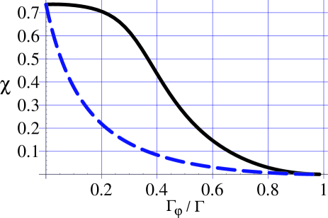
Figure 3: Quantum efficiency ratio $\chi$ versus $\Gamma_{\varphi}/\Gamma$ for the resonant level model, in the large-voltage “cotunneling” limit: $\mu_{L}-\mu_{R}=100\Gamma$, and $\varepsilon_{d}=\mu_{L}+\Gamma$. The long-dashed blue curve corresponds to the dephasing voltage probe model, while the solid black curve corresponds to the slow random potential model (with $\Gamma_{\varphi}\rightarrow\lambda_{\varphi}$). Despite the large voltage, $\chi$ is still suppressed to zero by dephasing in both models; note also the large difference between the two models.

IV Dephasing From a Fluctuating Potential

IV.1 General setup

We now consider an alternate model of dephasing in which the resonant level detector is subject to a random, Gaussian-distributed, time-dependent potential. This model represents the classical (high-temperature) limit of dephasing induced by a bath of oscillators (e.g. phonons), and is attractive as it allows a simple semiclassical interpretation of the influence of dephasing on noise. It also allows one to make a clear distinction between pure dephasing effects and inelastic scattering. Surprisingly, we find that for noise properties, dephasing from a fluctuating random potential is not completely equivalent to any of the voltage probe models, even if one chooses a “slow” potential which does not give rise to inelastic effects; one finds a reasonable agreement between the models only in the small voltage regime. The upshot of the analysis is that the noise properties and detector efficiency of the resonant level model is sensitive both to the degree of detector coherence and the nature of the dephasing source. Study of the random potential model also helps elucidate the origin of the two contributions to the charge noise found in voltage probe models (c.f. Eq. (26)).

Note that a model somewhat similar to that considered here was used by Davies et. al DaviesIncRLM to study the effect of dephasing on current noise in a double tunnel-junction structure. Unlike the present study, they focused on the large voltage regime $eV\gg\Gamma$, and could not consider the effect of varying the timescale of the random potential. The effect of a fluctuating potential on current noise in a mesoscopic interferometer was also recently studied by Marquardt et. al. Marquardt . The situation here is quite different, as the scattering has a marked energy dependence, and we are also interested in the back-action charge fluctuations.

The time-dependent Hamiltonian for the system is:

$$H(t) = \left[\varepsilon_{d}+\eta(t)\right]d^{{\dagger}}d^{\phantom{\dagger}}+\sum_{\alpha=L,R}\int_{-D}^{D}d\epsilon\left[\epsilon\cdot c^{{\dagger}}_{\alpha}(\epsilon)c^{\phantom{\dagger}}_{\alpha}(\epsilon)\right]+$$ (33)

$$\sum_{\alpha=L,R}\sqrt{\frac{\Gamma_{\alpha}}{2\pi}}\int d\epsilon\left[d^{{\dagger}}c^{\phantom{\dagger}}_{\alpha}(\epsilon)+c^{{\dagger}}_{\alpha}(\epsilon)d^{\phantom{\dagger}}\right]$$

Assuming that the conduction electron bandwidth $D$ is the largest scale in the problem, we may solve the Heisenberg equations. Setting $\hbar=1$, we find:

$$d(t)=\int dt^{\prime}G^{R}(t,t^{\prime})\sum_{\alpha}\sqrt{\frac{\Gamma_{\alpha}}{2\pi}}\int d\varepsilon e^{-i\varepsilon t^{\prime}}\tilde{c}^{\phantom{\dagger}}_{\alpha}(\varepsilon)$$ (34)

where

$$G^{R}(t,t^{\prime}) = -i\theta(t-t^{\prime})e^{-\Gamma_{0}(t-t^{\prime})/2}e^{-i\varepsilon_{d}(t-t^{\prime})}\times$$ (35)

$$\exp\left(-i\int_{t^{\prime}}^{t}d\tau\eta(\tau)\right)$$

and where the $\tilde{c}_{\alpha}(\varepsilon)$ operators describe conduction electrons in the leads in the absence of tunneling. Expectations of the $\tilde{c}_{\alpha}$ operators obey Wick’s theorem, and are given in terms of the lead distribution functions in the usual manner. We will assume throughout that the noise $\eta(t)$ is stationary and Gaussian with an auto-correlation function $J(\tau)$:

$$\langle\eta(t)\eta(t^{\prime})\rangle=J(t-t^{\prime})=J(t^{\prime}-t)$$ (36)

Note that whereas voltage probe models are essentially characterized by a single energy scale $\Gamma_{\varphi}$, here the bandwidth and magnitude of $J(t=0)$ give two distinct scales.

IV.1.1 Average current

Defining the current in lead $\alpha$ as the time derivative of the particle number in lead $\alpha$ yields:

$$I_{\alpha}(t)/e=-\Gamma_{\alpha}d^{\dagger}(t)d(t)+i\sqrt{\frac{\Gamma_{\alpha}}{2\pi}}\int d\omega\left[e^{i\omega t}\tilde{c}^{{\dagger}}_{\alpha}(\omega)d(t)-\textrm{ h.c. }\right]$$ (37)

Taking the expectation of Eq. (37) for the current in the right lead, we find:

$$\langle I_{\alpha}(t)\rangle = -e\Gamma_{\alpha}\int d\omega\int_{-\infty}^{\infty}dt_{0}\Bigg{[}\Gamma_{0}\bar{f}(\omega)\int_{-\infty}^{\infty}dt_{b}G^{A}(t_{b},t;\omega)G^{R}(t,t_{0};\omega)+2f_{\alpha}(\omega)\textrm{ Im}G^{R}(t,t_{0};\omega)\Bigg{]}$$ (38)

where $\bar{f}$ is defined in Eq. (29), and the additional argument $\omega$ in $G^{R/A}$ indicates that one should shift $\varepsilon_{d}\rightarrow\varepsilon_{d}-\omega$ in Eq. (35). Given the simple form of $G^{R}(t,t^{\prime})$, there is an optical theorem which relates these two contributions for arbitrary $\eta(t)$:

$$\int dt_{a}\int dt_{b}G^{A}(t_{b},t;\omega)G^{R}(t,t_{a};\omega)=$$ (39)

$$-2\int d{t_{0}}e^{-\Gamma_{0}t_{0}}\int d\tau\textrm{ Im }G^{R}(t-t_{0},t-t_{0}-\tau;\omega)$$

Using this to simplify Eq. (38) and then averaging over the random potential $\eta$ yields:

$$\langle\langle I_{R}\rangle\rangle_{\eta}= \frac{e}{2\pi}\frac{2\Gamma_{R}\Gamma_{L}}{\Gamma_{0}}\int d\omega(f_{R}(\omega)-f_{L}(\omega))$$ (40)

$$\int_{0}^{\infty}d\tau\textrm{ Im }\langle G^{R}(\tau,0;\omega)\rangle_{\eta}$$

We have used the fact that the $\eta$-averaged value of $G^{R}$ is invariant under time-translation. Eq. (40) for $\langle I\rangle$ is identical to the expression emerging from the dephasing voltage probe model (c.f. Eq. (30)), with the $\eta$-averaged Green function playing the role of the “dephased” Green function $\tilde{G}^{R}$ in the latter model. On a heuristic level, Eq. (40) indicates that tunneling processes with different dwell times $\tau$ on the level contribute to $\langle I\rangle$; the random phases picked up during these events will cause a suppression of the current.

Averaging the $\eta$ dependent parts of $G^{R}$ yields:

$$\langle G^{R}(\tau)\rangle_{\eta}= e^{-i\varepsilon_{d}\tau}e^{-\Gamma_{0}\tau/2}\times$$

$$\exp\left(-\frac{1}{\pi}\int_{-\infty}^{\infty}d\omega\frac{\sin(\omega t/2)^{2}}{\omega^{2}}J(\omega)\right)$$

Not surprisingly, the factor in $\langle G^{R}\rangle$ arising from the averaging has an identical form to what is encountered when studying the dephasing of a spin coupled to a random potential or to a bosonic bath.

IV.1.2 Charge noise

In general, the noise in a quantity $X$ in the fluctuating potential model will have two distinct sources:

$$\textrm{Var}\left[X^{2}\right]=\Big{\langle}\left[\langle X^{2}\rangle-\langle X\rangle^{2}\right]\Big{\rangle}_{\eta}+\left(\Big{\langle}\langle X\rangle^{2}\Big{\rangle}_{\eta}-\langle\langle X\rangle\rangle_{\eta}^{2}\right)$$ (42)

The first term describes the intrinsic noise for each given realization of $\eta(t)$, whereas the second describes the classical fluctuation of the average value of $X$ from realization to realization. In what follows, we will focus on the first, more intrinsic effect; this corresponds to an experiment where the noise (i.e. variance) is calculated for each realization of $\eta(t)$, and is only then averaged over different realizations. Note that the neglected classical contribution to the noise (i.e. the second term in Eq. (42)) is positive definite; including it will only push the system further from the quantum limit.

Noting that here, $Q(t)\equiv d^{{\dagger}}(t)d(t)$, we find using Eq. (34):

$$S_{Q} \equiv 2\int_{-\infty}^{\infty}dt\Big{\langle}\left[\langle Q(t)Q(0)\rangle-\langle Q(t)\rangle\langle Q(0)\rangle\right]\Big{\rangle}_{\eta}$$ (43)

$$= \frac{2e^{2}}{\pi^{2}}\int_{-\infty}^{\infty}dt\int_{-\infty}^{\infty}d\bar{\omega}\int_{-\infty}^{\infty}d(\Delta\omega)e^{i\Delta\omega t}\int_{0}^{\infty}d\tau_{1}\int_{0}^{\infty}d\tau_{2}$$

$$\bar{f}(\bar{\omega}+\Delta\omega/2)\left(1-\bar{f}(\bar{\omega}-\Delta\omega/2)\right)e^{-i\Delta\omega(\tau_{1}-\tau_{2})/2}$$

$$\Big{\langle}\textrm{ Im }G^{R}(t,t-\tau_{1};\bar{\omega})\textrm{ Im }G^{R}(0,-\tau_{2};\bar{\omega})\Big{\rangle}_{\eta}$$

We have used the optical theorem of Eq. (39) to express $S_{Q}$ in terms of a product of two (as opposed to four) Green functions. Similar to Eq. (40) for the current, Eq. (43) for $S_{Q}$ may be given a simple heuristic interpretation. The first factor of $G^{R}$ in Eq. (43) yields the amplitude of an event where an electron leaves the level at time $t$ after having spent a time $\tau_{1}$ on the level, while the second describes a process where an electron leaves the level at time $0$ after a dwell time $\tau_{2}$. Eq. (43) thus expresses the charge noise as a sum over pairs of tunneling events occurring at different times. Unlike the average current (c.f. Eq. (38)), the charge noise is sensitive to interference between tunnel events which have different exit times from the level.

It is useful to write the Green function factor in Eq. (43) as:

$$\Big{\langle}\textrm{ Im }G^{R}(t,t-\tau_{1};\bar{\omega})\textrm{ Im }G^{R}(0,-\tau_{2};\bar{\omega})\Big{\rangle}_{\eta}=$$

$$\textrm{Re }\frac{W^{D}(t;\tau_{1},\tau_{2})-W^{I}(t;\tau_{1},\tau_{2})}{2}$$ (44)

where

$$W^{D}(t;\tau_{1},\tau_{2}) = \Big{\langle}G^{R}(t,t-\tau_{1})G^{A}(0,-\tau_{2})\Big{\rangle}$$ (45a)

$$W^{I}(t;\tau_{1},\tau_{2}) = \Big{\langle}G^{R}(t,t-\tau_{1})G^{R}(0,-\tau_{2})\Big{\rangle}$$ (45b)

Similar to standard disorder-averaged calculations, we have both a “diffuson” ($W^{D}$) and an “interference” ($W^{I}$) contribution. Averaging over the random potential yields:

$$W^{D/C}(t;\tau_{1},\tau_{2})=e^{-i(\varepsilon_{d}-\bar{\omega})(\tau_{1}\mp\tau_{2})}e^{-\Gamma_{0}(\tau_{1}+\tau_{2})/2}$$

$$\exp\left[-\frac{1}{2}\int_{-\infty}^{\infty}dt_{1}\int_{-\infty}^{\infty}dt_{2}\chi_{\mp}(t_{1})\chi_{\mp}(t_{2})J(t_{1}-t_{2})\right]$$ (46)

where

$$\chi_{\pm}(t) = \chi_{[t-\tau_{1},t]}(t)\pm\chi_{[-\tau_{2},0]}(t)$$ (47a)

$$\chi_{[t_{i},t_{f}]}(t) = \theta(t-t_{i})-\theta(t-t_{f})$$ (47b)

In what follows, it is useful to make the shift $t\rightarrow t+(\tau_{1}-\tau_{2})/2$ in Eq. (43). Simplifying, and using the fact that the $\eta$-averaged Green function is time-translation invariant, we then have:

$$W^{D}(t;\tau_{1},\tau_{2}) = C(t;\tau_{1},\tau_{2})\left[\langle G^{R}(\tau_{1})\rangle\langle G^{A}(\tau_{2})\rangle\right]$$ (48a)

$$W^{I}(t;\tau_{1},\tau_{2}) = \frac{\left[\langle G^{R}(\tau_{1})\rangle\langle G^{R}(\tau_{2})\rangle\right]}{C(t;\tau_{1},\tau_{2})}$$ (48b)

with

$$C(t;\tau_{1},\tau_{2}) = \exp\Big{[}\int_{-\infty}^{\infty}dt_{1}\int_{-\infty}^{\infty}dt_{2}$$ (49)

$$\chi_{[t-\frac{\tau_{1}+\tau_{2}}{2},t+\frac{\tau_{1}-\tau_{2}}{2}]}(t_{1})\chi_{[-\tau_{2},0]}(t_{2})J(t_{1}-t_{2})\Big{]}$$

$$= \exp\Bigg{[}\frac{2}{\pi}\int_{-\infty}^{\infty}d\omega J(\omega)$$

$$\times\frac{\sin(\omega\tau_{1}/2)\sin(\omega\tau_{2}/2)}{\omega^{2}}\cos\omega t\Bigg{]}$$

Eq. (46) indicates that the general effect of the random potential is to suppress the contribution of each pair of tunnel events to $S_{Q}$. The correlation between the random phases acquired by each of the two events plays a central role, and is described by the factor $C(t;\tau_{1},\tau_{2})$, where $\tau_{1},\tau_{2}$ are the dwell times of the two events, and $t$ is the difference in exit times. Eq. (49) gives a simple expression for $C(t;\tau_{1},\tau_{2})$ in terms of the spectral density of the random potential. The existence of phase correlations allows pairs of tunnel events to interfere constructively when contributing to the diffuson contribution; thus, as can be seen in Eqs. (48), phase correlations tend to enhance the diffuson contribution relative to the interference contribution.

In addition, the phase correlation factor $C(t;\tau_{1},\tau_{2})$ is the only $t$ dependent factor remaining in the expression for $S_{Q}$ after $\eta$ averaging. Thus, it will completely determine the contribution of inelastic processes to the charge noise $S_{Q}$ (i.e. terms with $\Delta\omega\neq 0$ in Eq. (43)). Such processes correspond to the absorption or emission of energy by the random potential. Note the formal similarity between the correlation kernel $C(t;\tau_{1},\tau_{2})$ in Eq. (43), and the kernel appearing in the $P(E)$ theory describing the effect of environmental noise on electron tunneling PEReference . Here, not surprisingly, the probability of an inelastic transition depends on the dwell times $\tau_{1}$, $\tau_{2}$ of the two tunnel events.

We can now straightforwardly identify the “pure dephasing” (i.e. elastic) contribution to $S_{Q}$ for an arbitrary $J(\omega)$ by keeping only the $t$-independent part of $C(t;\tau_{1},\tau_{2})$ when evaluating Eq. (43). This is equivalent to replacing $C(t;\tau_{1},\tau_{2})$ by $C(t\rightarrow\infty;\tau_{1},\tau_{2})$ in Eq. (43). We thus define:

$$S_{Q}\big{|}_{elast} = \frac{2e^{2}}{\pi}\int_{-\infty}^{\infty}d\omega\bar{f}(\omega)(1-\bar{f}(\omega))\int d\tau_{1}\int d\tau_{2}$$

$$\textrm{Re }\left[W^{D}(t\rightarrow\infty;\tau_{1},\tau_{2})-W^{I}(t\rightarrow\infty;\tau_{1},\tau_{2})\right]$$

If, in addition, we have the reasonable result that there are no phase correlations in the long time-separation limit (i.e. $C(t;\tau_{1},\tau_{2})\rightarrow 1$ as $t\rightarrow\infty$), the elastic contribution becomes:

$$S_{Q}\big{|}_{elast}=\frac{4e^{2}}{\pi}\int_{-\infty}^{\infty}d\omega\bar{f}(\omega)(1-\bar{f}(\omega))\Big{\langle}\textrm{Im }G^{R}(\omega)\Big{\rangle}^{2}$$ (51)

This expression for the elastic contribution to $S_{Q}$ is identical to what is obtained for the intrinsic charge fluctuations $[S_{Q}]_{bare}$ in the dephasing voltage probe model (c.f. Eq. (31)), if we associate the $\eta$-averaged Green function with the dephased Green function $\tilde{G}^{R}$ in the latter model. Recall that the in the voltage probe model, the intrinsic contribution $[S_{Q}]_{bare}$ arises from fluctuations of the total current incident on the level, and is independent of fluctuations of the probe voltage. We thus have that if there are no long-time phase correlations, the purely elastic effect of a random potential is captured (in form) by the intrinsic charge fluctuations in the dephasing voltage probe model. Note that in Eq. (51) both the interference and diffuson terms contribute equally. The lack of any phase correlations implies that there is no relative enhancement of $W^{D}$ over $W^{I}$.

Finally, we may define a purely inelastic contribution to $S_{Q}$ for an arbitrary $J(\omega)$ by simply subtracting off the elastic contribution defined in Eq. (IV.1.2) from the full expression for $S_{Q}$. We find:

$$S_{Q}|_{inelast} = \frac{2e^{2}}{\pi}\int_{-\infty}^{\infty}d\bar{\omega}\int_{-\infty}^{\infty}d(\Delta\omega)\int_{0}^{\infty}d\tau_{1}\int_{0}^{\infty}d\tau_{2}\bar{f}(\bar{\omega}+\Delta\omega/2)\left(1-\bar{f}(\bar{\omega}-\Delta\omega/2)\right)$$

$$\textrm{ Re}\Bigg{[}P_{D}(\Delta\omega;\tau_{1},\tau_{2})\Big{\langle}G^{R}(\tau_{1};\bar{\omega})\Big{\rangle}_{\eta}\Big{\langle}G^{A}(\tau_{2};\bar{\omega})\Big{\rangle}_{\eta}-P_{I}(\Delta\omega;\tau_{1},\tau_{2})\Big{\langle}G^{R}(\tau_{1};\bar{\omega})\Big{\rangle}_{\eta}\Big{\langle}G^{R}(\tau_{2};\bar{\omega})\Big{\rangle}_{\eta}\Bigg{]}$$

where we have defined the real-valued functions:

$$P_{D/I}(\Delta\omega;\tau_{1},\tau_{2})=$$ (53)

$$\int dt\frac{e^{i\Delta\omega t}}{2\pi}\Big{[}C(t;\tau_{1},\tau_{2})^{\pm 1}-C(t\rightarrow\infty;\tau_{1},\tau_{2})^{\pm 1}\Big{]}$$

Though they are not necessarily positive definite, the functions $P_{D/I}(\Delta\omega;\tau_{1},\tau_{2})$ may be interpreted as the quasi-probability of obtaining an inelastic contribution of size $\Delta\omega$ from (respectively) the diffuson or interference contribution.

IV.1.3 Current noise

We again focus on the “intrinsic” fluctuations (e.g. the first term in Eq. (42)) and ignore the additional contribution to the current noise arising from variations of $\langle I\rangle$ in different realizations of the random potential $\eta$. Similar to the case of the charge noise, the current noise $S_{I}$ may be expressed in terms of products of $G^{R}$ and $G^{A}$ at different times. Also, a direct calculation shows that current conservation holds for the fluctuations: the current noise is independent of the lead in which it is calculated. Writing the current noise as:

$$S_{I} = \frac{2e^{2}\Gamma_{L}\Gamma_{R}}{2\pi^{2}}\sum_{\alpha,\beta=L,R}\int_{-\infty}^{\infty}d\bar{\omega}\int_{-\infty}^{\infty}d(\Delta\omega)\int_{0}^{\infty}d\tau_{1}\int_{0}^{\infty}d\tau_{2}$$ (54)

$$e^{i\Delta\omega t}\left(f_{\alpha}(\bar{\omega}+\Delta\omega/2)\right)\left(1-f_{\beta}(\bar{\omega}-\Delta\omega/2)\right)$$

$$\times e^{-i\Delta\omega(\tau_{1}-\tau_{2})/2}\textrm{ Re}\left[\delta_{\alpha\beta}S_{I}^{d}+(1-\delta_{\alpha\beta})S_{I}^{od}\right]$$

we find after averaging:

$$S_{I}^{d}(t;\tau_{1},\tau_{2}) = \frac{2\Gamma_{L}\Gamma_{R}}{\Gamma_{0}^{2}}\left(W^{D}-W^{I}\right)$$ (55)

$$S_{I}^{od}(t;\tau_{1},\tau_{2}) = \frac{\Gamma_{L}^{2}+\Gamma_{R}^{2}}{\Gamma_{0}^{2}}W^{D}+\frac{2\Gamma_{L}\Gamma_{R}}{\Gamma_{0}^{2}}W^{I}.$$ (56)

Similar to the charge noise, the current noise results from the interference between pairs of tunnel events, and may be expressed in terms of the diffuson and interference terms defined in Eqs. (45) (we have suppressed their time arguments above for clarity). Unlike the charge noise, we see that for the off-diagonal fluctuations ($S_{I}^{od}$), the diffuson and interference term enter with different coefficients. Note that in the zero voltage case, the interference term $W^{I}$ does not contribute:

$$\left[\delta_{\alpha\beta}S_{I}^{d}+(1-\delta_{\alpha\beta})S_{I}^{od}\right]\rightarrow W^{D}(t;\tau_{1},\tau_{2})$$ (57)

Elastic and inelastic contributions to $S_{I}$ may be identified in the same way as was done for $S_{Q}$.

IV.2 Results from the slow random potential model

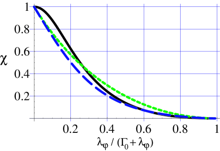
Figure 4: Solid black curve: quantum efficiency ratio $\chi$ versus dephasing strength for the slow random potential model, in the limit $eV\rightarrow 0$. We have assumed symmetric couplings $\Gamma_{L}=\Gamma_{R}$, and have chosen $\varepsilon_{d}$ so as to maximize the gain. For comparison, the long-dashed blue curve (short-dashed red curve) corresponds to the dephasing (inelastic) voltage probe model, with $\lambda_{\varphi}\rightarrow\Gamma_{\varphi}$.

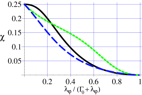
Figure 5: Quantum efficiency ratio $\chi$ versus dephasing strength for the slow random potential, in the limit $eV\rightarrow 0$ and for $\Gamma_{L}\gg\Gamma_{R}$. We have chosen $\varepsilon_{d}$ so as to maximize the gain. Curves labelled as in Fig. 4.

Similar to Ref. Marquardt, , we will consider in what follows two limiting cases for the spectral density $J(\omega)$. The first is that of a “slow” random potential, where the bandwidth $\Omega$ of $J(\omega)$ is much smaller than the frequency scales of interest, i.e..

$$\Omega\ll\Gamma_{0},\varepsilon_{d}-\mu_{L},\varepsilon_{d}-\mu_{R},|\mu_{L}-\mu_{R}|$$ (58)

This allows us to make the approximation

$$J(t)\rightarrow J(t=0)$$ (59)

Inelastic effects should be minimal in this limit, and thus one might expect results which are similar to the dephasing voltage probe model.

For the averaged Green function, the approximation of Eq. (59) in Eq. (IV.1.1) yields:

$$\langle G^{R}(\tau)\rangle=e^{-i\varepsilon_{d}\tau}e^{-\Gamma_{0}\tau/2}e^{-(\lambda_{\varphi}t)^{2}/2}$$ (60)

where

$$\lambda_{\varphi}=\sqrt{J(t\rightarrow 0)}.$$ (61)

Plugging this into Eq. (40) yields a Voit lineshape (i.e. a convolution of a Gaussian and a Lorentzian):

$$\langle\langle I\rangle\rangle = \frac{e}{2\pi}\frac{2\Gamma_{R}\Gamma_{L}}{\Gamma_{0}}\int d\omega(f_{L}(\omega)-f_{R}(\omega))$$ (62)

$$\int d\omega^{\prime}\left(\frac{e^{-\omega^{\prime 2}/(2\lambda_{\varphi}^{2})}}{\sqrt{2\pi\lambda_{\varphi}^{2}}}\right)\frac{\Gamma_{0}/2}{(\varepsilon_{d}-\omega-\omega^{\prime})^{2}+(\Gamma_{0})^{2}/4}$$

$$= \int d\omega^{\prime}\left(\frac{e^{-\omega^{\prime 2}/(2\lambda_{\varphi}^{2})}}{\sqrt{2\pi\lambda_{\varphi}^{2}}}\right)\langle I\rangle\Big{|}_{\varepsilon_{d}\rightarrow\varepsilon_{d}-\omega^{\prime}}$$

In the “slow” limit, $\langle I\rangle$ is inhomogeneously broadened– while the random potential $\eta(t)$ is essentially constant for each event where an electron tunnels on and then off the level, it does fluctuates from event to event. The effect of $\eta$ on $\langle I\rangle$ can thus be mimicked by simply averaging over a Gaussian distribution of level positions $\varepsilon_{d}$. As a result, the effect of dephasing is not simple lifetime broadening, and the conductance lineshape is manifestly non-Lorentzian; this is in contrast to the voltage probe models. Nonetheless, if we associate $\lambda_{\varphi}$ with $\Gamma_{\varphi}$, the height and width of the resonance described by Eq. (62) for $\langle I\rangle$ is similar to that obtained in the voltage probe model.

Turning to the noise for the “slow” random potential model, we remark again that we focus throughout this section on the intrinsic contribution to the noise defined by the first term in Eq. (42). We first calculate the phase correlation factor using Eq. (48b):

$$C(t;\tau_{1},\tau_{2})=\exp\left[\lambda_{\varphi}^{2}\tau_{1}\tau_{2}\right]$$ (63)

Again, $C(t;\tau_{1},\tau_{2})$ describes the correlations in the random phases acquired by two tunnel events (dwell times $\tau_{1},\tau_{2}$) with a time separation $t$. Here, $C(t;\tau_{1},\tau_{2})$ is independent of time, implying (as expected) only elastic contributions to $S_{Q}$ and $S_{I}$. However, the corresponding fact that phase correlations persist even at large time separations (i.e. $C(t\rightarrow\infty)\neq 1$) implies that the elastic contribution to $S_{Q}$ is not given by the simple result of Eq. (51). It follows that the charge noise in this limit cannot agree with the intrinsic charge noise $[S_{Q}]_{bare}$ (Eq. (31)) found in the dephasing voltage probe model.

One can simply relate the diffuson and interference contributions to the $\eta$-averaged Green function, resulting in:

$$S_{Q} = \frac{4e^{2}}{\pi\Gamma_{0}}\int d\omega\Big{[}\bar{f}(\omega)(1-\bar{f}(\omega))$$ (64)

$$\left(1-\Gamma_{0}\frac{\partial}{\partial\Gamma_{0}}\right)\langle-\textrm{Im }G^{R}(\omega)\rangle_{\eta}\Big{]}$$

The two terms in this expression correspond to the diffuson and interference contributions respectively. As can easily be verified, Eq. (64) is simply the charge noise of the fully coherent system (i.e. Eq. (51) at $\eta=0$) averaged over a Gaussian distribution of level positions; this is analogous to what was found for the average current. In the strong dephasing limit, $\langle G^{R}\rangle_{\eta}$ becomes independent of $\Gamma_{0}$, and we thus have at zero temperature (but arbitrary voltage):

$$S_{Q}=4\frac{|\langle I\rangle|}{(\Gamma_{0})^{2}}$$ (65)

This expression is identical to what is found in both the inelastic and elastic voltage probe models in the strong dephasing limit (c.f. Eq. (28)), and for small voltages, scales as $eV/(\lambda_{\varphi}\Gamma_{0})$. The correspondence to these voltage probe models is not surprising, as in the strong dephasing limit, the charge noise in these models is dominated by the fluctuations of the potential in the voltage probe. Not surprisingly, these fluctuations are equivalent to exposing the level directly to a slow, random potential.

Turning to the current noise $S_{I}$, we find at zero temperature:

$$S_{I} = \frac{2e^{2}\Gamma_{L}\Gamma_{R}}{\pi\Gamma_{0}}\int_{-\infty}^{\infty}d\bar{\omega}f_{L}(\bar{\omega})\left(1-f_{R}(\bar{\omega})\right)$$ (66)

$$\left[\frac{\Gamma_{L}^{2}+\Gamma_{R}^{2}}{\Gamma_{0}^{2}}+\frac{2\Gamma_{L}\Gamma_{R}}{\Gamma_{0}}\frac{\partial}{\partial\Gamma_{0}}\right]\langle-\textrm{ Im}G^{R}(\omega)\rangle_{\eta}$$

Taking the large dephasing limit ($\lambda_{\varphi}\gg\Gamma_{0}$) yields:

$$S_{I} \rightarrow 2e\left(\frac{\Gamma_{L}^{2}+\Gamma_{R}^{2}}{\Gamma_{0}^{2}}\right)\langle I\rangle$$ (67)

The Fano factor here has the familiar form corresponding to the shot noise of two classical Poisson processes in series, and agrees with the voltage probe result (c.f. Eq. (23)). Thus, we find that the slow random potential model and the dephasing voltage probe model agree both on the form of $S_{I}$ and $S_{Q}$ in the strong dephasing limit; this is despite the fact that they yield quite different conductance lineshapes.

Turning to the question of the quantum limit, shown in Figs. 4 and 5 is $\chi$ as function of dephasing strength for the “slow” random potential model at zero temperature and small voltage. The results obtained for $S_{I}$ and $S_{Q}$ suggest that at large dephasing strengths, $\chi$ in the slow potential model will be the same as that found in the dephasing voltage probe model. As seen in Figs. 4 and 5, we find that a reasonable correspondence holds even at moderate levels of dephasing . This does not however imply that the two models are always equilvaent. We have also calculated $\chi$ in the large voltage, “co-tunneling” limit considered by Averin AverinRLM , see Fig. 3. Here, there is a marked quantitative difference between the slow potential model and the dephasing voltage probe model, with $\chi$ being suppressed more quickly by dephasing in the latter model. Again, we see that both the nature of the dephasing source as well as the strength of dephasing influences the suppression of $\chi$.

The departure from the quantum limit in the fluctuating random potential model may be understood as it was in the dephasing voltage probe model (see text following Eq. (28))– there is a classical uncertainty in the system stemming from the source of dephasing; this uncertainty in turn leads to extraneous noise in both $I$ and $Q$ which takes one away from the quantum limit.

Finally, it is instructive to look at the results of this section while retaining a small bandwidth $\Omega$ for the spectral density $J(\omega)$. This will give further insight on the contribution $[S_{Q}]_{class}$ (c.f. Eq. (26)) to the charge noise in the voltage probe models, a contribution arising from fluctuations of the probe voltage. At small but finite bandwidth $\Omega$, the phase correlation factor will be given to a good approximation by:

$$C(t;\tau_{1},\tau_{2})=\exp\left[\lambda_{\varphi}^{2}\tau_{1}\tau_{2}e^{-\Omega|t|}\right]$$ (68)

For long times $|t|\gg 1/{\Omega}$, phase correlations will vanish, and the elastic contribution to $S_{Q}$ will again be given by Eq. (51) as opposed to Eq. (64). However, the presence of a small but finite bandwidth implies that there will now also exist an inelastic contribution to $S_{Q}$ (c.f. Eq. (IV.1.2)), corresponding to small energy transfers $\Delta\omega\sim\Omega$. The quasi-probability $P(\Delta\omega;\tau_{1},\tau_{2})$ for having an inelastic event will be given by (c.f. Eq. (53)):

$$P_{D/I}(\Delta\omega;\tau_{1},\tau_{2})=\frac{1}{\pi}\sum_{n=1}^{\infty}\frac{\left(\lambda_{\varphi}\tau_{1}\tau_{2}\right)^{n}}{n!}\frac{n\Omega}{(\Delta\omega)^{2}+(n\Omega)^{2}}$$ (69)

For typical dwell times $\lambda_{\varphi}^{2}\tau_{1}\tau_{2}$ is order unity, and thus the only significant contribution to the sum in Eq. (69) will come from the first few terms. Further, note that in Eq. (IV.1.2) for the inelastic contribution to $S_{Q}$, $\Delta\omega$ appears only in the distribution functions of the leads. Thus, since by assumption we have $eV,\Gamma_{0}\gg\Omega$, we may safely replace the Lorentzians in the above expression by delta functions, and the inelastic contribution may be accurately represented by an elastic one:

$$P_{D/I}(\Delta\omega;\tau_{1},\tau_{2})\rightarrow\delta(\Delta\omega)\left(C(t=0;\tau_{1},\tau_{2})^{\pm 1}-1\right)$$ (70)

In the case of $S_{Q}$, combining this “quasi-elastic” contribution with the pure elastic contribution given by Eq. (51) results again in Eq. (64), which was found above by taking the $\Omega\rightarrow 0$ limit from the outset. We thus see that the slow potential model includes the contribution from inelastic events involving a small energy transfer $\sim\Omega$; keeping only purely elastic contributions would yield the result of Eq. (51) for $S_{Q}$. As already noted, the purely elastic contribution coincides with the intrinsic contribution to the charge noise ($[S_{Q}]_{bare}$) found in the dephasing voltage probe model. It thus follows that the “quasi-elastic” contribution in the random potential model (i.e. stemming from Eq. (69)) corresponds to the contribution $[S_{Q}]_{class}$ in the voltage probe model (i.e. charge fluctuations induced by potential fluctuations in the probe, c.f. Eq. (32)).

IV.3 Results from the fast random potential model

The second limiting case of the random potential model is that of a “fast” random potential, where $J(\omega)$ is flat on the frequency scales of interest. This will allow us to make the replacement:

$$J(\omega)\rightarrow J(\omega=0)$$ (71)

A necessary requirement for the “fast” limit is that the characteristic bandwidth of the random potential $\Omega$ is much larger than the frequency scales of interest (i.e. reverse the inequality in Eq. (58)). Given this large bandwidth $\Omega$, we expect that inelastic contributions to $S_{Q}$ and $S_{I}$ will be important; this makes it unlikely that the total current or charge noise in this limit will agree with either of the voltage probe models. In what follows, we will consider separately the elastic and inelastic contributions to the noise.

Turning first to the average current in the presence of a “fast” random potential, Eq. (IV.1.1) yields:

$$\langle G^{R}(\tau)\rangle=e^{-i\varepsilon_{d}\tau}e^{-(\Gamma_{0}+\Gamma_{\varphi})\tau/2}$$ (72)

where

$$\Gamma_{\varphi}=J(\omega\rightarrow 0)$$ (73)

Thus, for the average Green function and average current, the effect of a “fast” random potential is just a simple lifetime broadening, identical to the situation in the voltage probe models. As a result, Eq. (40) yields the same Lorentzian result for $\langle I\rangle$ as the dephasing voltage probe model, Eq. (30). Note that for strong dephasing ($\Gamma_{\varphi}\gg\Gamma_{0}$), the approximation of Eq. (71) is valid only if $\Omega\gg\Gamma_{\varphi}$ in addition to the reversed-ineqality of Eq. (58). If this is not true, the contribution from short times in Eq. (40) will dominate, and one will not obtain a Lorentzian form for the average current (instead, the results for a “slow” random potential, discussed in the previous subsection, will apply).

We turn next to the calculation of $S_{Q}$ and $S_{I}$ for a “fast” random potential. We find that the factor $C(t;\tau_{1},\tau_{2})$ (c.f. Eq. (49)) describing the correlation between the random phases of a pair of tunnel events is given by:

$$C(t;\tau_{1},\tau_{2})=\exp\left[\Gamma_{\varphi}\tau_{overlap}\right]$$ (74)

where $\tau_{overlap}$ is the overlap between the two time intervals describing the tunneling events (i.e. $[t-\tau_{1},t]$ and $[0-\tau_{2},0]$), and $\Gamma_{\varphi}$ is defined in Eq. (73). As was anticipated in the discussion prior to Eq. (51), correlations in phase between the two tunnel events are important only if the time separation $t$ is sufficiently small. The correlations vanish as $t\rightarrow\infty$ (i.e. $C\rightarrow 1$), and thus the elastic contribution to $S_{Q}$ is given by Eq. (51). As with the result for $\langle I\rangle$, this expression agrees exactly with the dephasing voltage probe result of Eq. (31). However, in sharp contrast, the elastic contribution to $S_{I}$ deviates strongly from the voltage probe model. At $T=0$, we find for the elastic contribution:

$$S_{I}\big{|}_{elast}=\frac{2e^{2}}{2\pi}\Gamma_{L}\Gamma_{R}\int_{\mu_{R}}^{\mu_{L}}d\omega\left|\langle G^{R}(\omega)\rangle\right|^{4}\left[\omega^{2}+\Gamma^{2}\left(\frac{\Gamma_{L}-\Gamma_{R}}{2\Gamma_{0}}\right)^{2}\right]$$ (75)

Taking the strong dephasing limit $\Gamma_{\varphi}\gg\Gamma_{0}$, this yields a vanishing Fano factor:

$$f_{elast}\equiv\frac{S_{I}\big{|}_{elast}}{2e\langle I\rangle}\propto\frac{\Gamma_{0}}{\Gamma_{\varphi}}$$ (76)

In contrast, the voltage probe models yield a non-vanishing Fano factor in the incoherent limit, given by the classical expression of Eq. (23).

We turn now to the inelastic contributions to $S_{I}$ and $S_{Q}$ which are non-vanishing even at zero temperature and zero voltage. These inelastic contributions always increase the noise in the fluctuating potential model, while the opposite is found in voltage probe models: the inelastic version of the voltage probe model yields smaller values of $S_{Q}$ and $S_{I}$ than the purely elastic version. The inelastic contributions will be determined by the quasi-probabilities $P_{D/I}(\Delta\omega;\tau_{1},\tau_{2})$ defined in Eq. (53). We find

$$P_{D/I}(\Delta\omega;\tau_{1},\tau_{2}) = \frac{1}{\pi}\frac{\Gamma_{\varphi}}{(\Delta\omega)^{2}+\Gamma_{\varphi}^{2}}\Bigg{[}\frac{\Gamma_{\varphi}}{\Delta\omega}\left(e^{\pm\Gamma_{\varphi}\tau_{<}}\sin\left(\frac{\Delta\omega(\tau_{>}-\tau_{<})}{2}\right)-\sin\left(\frac{\Delta\omega(\tau_{>}+\tau_{<})}{2}\right)\right)$$ (77)

$$\pm\left(e^{\pm\Gamma_{\varphi}\tau_{<}}\cos\left(\frac{\Delta\omega(\tau_{>}-\tau_{<})}{2}\right)-\cos\left(\frac{\Delta\omega(\tau_{>}+\tau_{<})}{2}\right)\right)\Bigg{]}$$

Here, $\tau_{>}$ ($\tau_{<}$) is the greater (lesser) of $\tau_{1},\tau_{2}$. As expected, inelastic processes involving energy transfers $\Delta\omega\simeq\Gamma_{\varphi}$ can make a sizeable contribution to $S_{Q}$. In the strong dephasing limit ($\Gamma_{\varphi}\gg\Gamma_{0}$), these inelastic processes are an unavoidable consequence of having a Lorentzian form for the average current, as this requires a noise bandwidth $\Omega\gg\Gamma_{\varphi}$. In the strong dephasing limit, we find the simple result:

$$S_{Q}|_{inelastic} = \frac{2e^{2}}{\pi^{2}}\frac{1}{\Gamma_{0}}\int d\omega_{1}\int d\omega_{2}\bar{f}(\omega_{1})(1-\bar{f}(\omega_{2}))$$ (78)

$$\langle\textrm{Im }G^{R}(\omega_{1})\rangle_{\eta}\langle\textrm{Im }G^{R}(\omega_{2})\rangle_{\eta}$$

In the small voltage, large dephasing limit, the inelastic contribution to $S_{Q}$ scales as $(1/\Gamma_{0})$, and is much larger than the elastic contribution, which scales as $eV/\Gamma_{\varphi}^{2}$.

Similarly for $S_{I}$, we find an inelastic contribution in the $V\rightarrow 0$ limit given by:

$$S_{I}\big{|}_{inelast} = \frac{2e^{2}}{2\pi}\frac{\Gamma_{L}\Gamma_{R}}{\Gamma_{0}}\int d\omega_{1}\int d\omega_{2}$$ (79)

$$\left[f(\omega_{1})(1-f(\omega_{2}))+(1-2f(\omega_{1}))\frac{df(\omega_{2})}{d\omega}eV\right]$$

$$\times\big{\langle}\textrm{Im }G^{R}(\omega_{1})\big{\rangle}\big{\langle}\textrm{Im }G^{R}(\omega_{2})\big{\rangle}$$

Unlike the elastic contribution, this term does not vanish in the strong dephasing limit.

Table 1: Synopsis of results for the various dephasing models, for the limit of small voltage ($eV\ll\Gamma$) and large dephasing ($\Gamma_{0}/\Gamma\rightarrow 0$). The classical Fano factor $f_{classical}$ appearing in the third column is defined in Eq. (23). For the inelastic and dephasing voltage probe models, we distinguish the intrinsic contribution to $S_{Q}$ from that arising from fluctuations of the probe voltage.

Dephasing Source	$\langle dI/dV\rangle$	$S_{I}=2ef\langle I\rangle$	$S_{Q}$	$\chi$
“pure escape” voltage probe	Lorentzian	$\frac{1}{2}\leq f\leq 1$	$\propto\frac{\Gamma_{0}}{\Gamma}\rightarrow 0$	$\frac{1}{2f}\frac{(\mu-\varepsilon_{d})^{2}}{(\mu-\varepsilon_{d})^{2}+\Gamma^{2}/4}$
Inelastic voltage probe	Lorentzian	$f\rightarrow f_{classical}$	$[S_{Q}]_{bare}\propto\frac{\Gamma_{0}}{\Gamma}\rightarrow 0$	$\propto\left(\frac{\Gamma_{0}}{\Gamma}\right)^{2}\rightarrow 0$
			$[S_{Q}]_{class}\rightarrow\frac{4\langle I\rangle}{(\Gamma_{0})^{2}}\propto\frac{\Gamma}{\Gamma_{0}}$
Dephasing voltage probe	Lorentzian	$f\rightarrow f_{classical}$	$[S_{Q}]_{bare}$ independent of $\frac{\Gamma_{0}}{\Gamma}$	$\propto\left(\frac{\Gamma_{0}}{\Gamma}\right)^{2}\rightarrow 0$
			$[S_{Q}]_{class}\rightarrow\frac{4\langle I\rangle}{(\Gamma_{0})^{2}}\propto\frac{\Gamma}{\Gamma_{0}}$
“Slow” fluctuating potential	Voit profile (c.f. Eq. 62)	$f\rightarrow f_{classical}$	$\frac{4\langle I\rangle}{(\Gamma_{0})^{2}}\propto\frac{\Gamma}{\Gamma_{0}}$	$\propto\left(\frac{\Gamma_{0}}{\Gamma}\right)^{2}\rightarrow 0$
“Fast” fluctuating potential	Lorentzian	voltage independent	voltage independent	$\propto\left(\frac{eV\Gamma_{0}}{\Gamma^{2}}\right)^{2}\rightarrow 0$

Finally, we turn to the issue of the quantum limit for the “fast” fluctuating potential model, in the small voltage limit. If one (rather unphysically) only retains the elastic contributions, we have that $\chi\sim 1$ even in the strong dephasing limit. This is due to the strong suppression of $S_{I}\big{|}_{elast}$. Keeping the inelastic terms, one finds instead that $\chi$ is greatly suppressed. In the strong dephasing limit, we have:

$$\chi\propto\left(\frac{eV}{\Gamma}\right)^{2}\left(\frac{\Gamma_{0}}{\Gamma}\right)^{2}$$ (80)

V Conclusions

We have studied the noise properties and detector efficiency of a mesoscopic resonant-level system subject to dephasing. We find that these properties are sensitive both to the degree of detector coherence (i.e. the ratio $\Gamma_{0}/\Gamma$) and to the nature of the dephasing source. This is in contrast to the average current, which is largely insensitive to the degree of coherence. Thus, even though one may have a well defined resonance in the average current, its suitability for use as a detector will depend strongly on its coherence properties.

We find that in general, different models of dephasing all lead to a suppression of the measurement efficiency $\chi$, though the rate at which this occurs depends on the model (see Figs. 1-5). The only exception to the above is dephasing arising from the “pure escape” voltage probe model. Here, $\chi$ may remain order unity even in the strong dephasing limit, a limit in which all transport involves entering the voltage probe and then leaving it incoherently. Though this result appears surprising, the “pure escape” model is unique among those considered, as there is no lost information associated with the dephasing source, nor is there any classical contribution to the detector noise arising from the detector being in a mixed (i.e. non-pure) state; this is why it is able to remain quantum limited in the fully incoherent limit. Among the more conventional voltage probe models, we find that $\chi$ is suppressed more quickly to zero by dephasing in the dephasing voltage probe model than in the inelastic voltage probe model (see Figs. 1 and 2). The differences between the models considered is summarized in Table 1.

Although the models considered here for dephasing may be regarded as describing to some extent the effect of interactions on the measurement efficiency of quantum detectors, it will be interesting to study this question in more general setups and in models in which strong interactions are directly included.

We thank S. Girvin and F. Marquadt for useful discussions, and M. Buttiker for a critical reading of the original manuscript and pointing out the importance of the second term in Eq. (26). This work was supported by the Keck foundation, and by the NSF under grant No. DMR-0084501.

References

- (1) S. A. Gurvitz, Phys. Rev. B 56, 15215 (1997).
- (2) I. L. Aleiner, N. S. Wingreen, and Y. Meir, Phys. Rev. Lett. 79, 3740 (1997)
- (3) Y. Levinson, Europhys. Lett. 39, 299 (1997)
- (4) E. Buks, R. Schuster, M. Heiblum, D. Mahalu, and V. Umansky, Nature (London) 391, 871 (1998).
- (5) L. Stodolsky, Phys. Lett. B 459, 193 (1999)
- (6) A. N. Korotkov and D. V. Averin, cond-mat/0002203.
- (7) D. V. Averin, quant-ph/0008114
- (8) Y. Makhlin et al., Phys. Rev. Lett. 85, 4578 (2000); ibid., Rev. Mod. Phys. 73, 357 (2001).
- (9) M. H. Devoret and R. J. Schoelkopf, Nature (London) 406, 1039 (2000).
- (10) A. N. Korotkov and D. V. Averin, Phys. Rev. B 64, 165310 (2001)
- (11) S. Pilgram and M. Büttiker, Phys. Rev. Lett. 89, 200401 (2002).
- (12) A. A. Clerk, S. M. Girvin and A. D. Stone, Phys. Rev. B 67, 165324 (2003).
- (13) D. V. Averin, cond-mat/0301524 (2003).
- (14) A. Shnirman, D. Mozyrsky and I. Martin, cond-mat/0311325 (2003).
- (15) M. Büttiker, Lecture Notes in Physics 547, 81 (2000) (cond-mat/9908116).
- (16) G. Seelig, S. Pilgram, A. N. Jordan and M. Büttiker, Phys. Rev. B 68, 161310 (2003).
- (17) D. Sprinzak, E. Buks, M. Heiblum and H. Shtrikman, Phys. Rev. Lett. 84, 5820 (2000).
- (18) D. V. Averin and V. Ya. Aleshkin, JETP Lett. 50, 367 (1989); ibid., Physica B 165 & 166, 949 (1990).
- (19) M-S. Choi, F. Plastina and R. Fazio, Phys. Rev. Lett. 87, 116601-1 (2001).
- (20) A. A. Clerk, S. M. Girvin, A. K. Nguyen, and A. D. Stone, Phys. Rev. Lett. 89, 176804 (2002)
- (21) Y. Nakamura , Y. A. Pashkin, and J. S. Tsai, Nature (London) 398, 786 (1999)
- (22) K. W. Lehnert, K. Bladh, L. F. Spietz, D. Gunnarsson, D. I. Schuster, P. Delsing, and R. J. Schoelkopf, Phys. Rev. Lett. 90, 027002 (2003)
- (23) C. M. Caves, Phys. Rev. D 26, 1817 (1982).
- (24) D. V. Averin, J. Appl. Phys. 73, 2593 (1993).
- (25) L. Y. Chen and C. S. Ting, Phys. Rev. B 43, 4534 (1991).
- (26) J. H. Davies, P. Hyldegaard, S. Hershfield and J. W. Wilkins, Phys. Rev. B 46, 9620 (1992).
- (27) Ya. M. Blanter and M. Büttiker, Phys. Rep. 336, 1 (2000).
- (28) M. Büttiker, IBM J. Res. Dev. 32, 63 (1988).
- (29) A. D. Stone and P. A. Lee, Phys. Rev. Lett. 54, 1196 (1985).
- (30) C. W. J. Beenakker, Rev. Mod. Phys. 69, 731 (1997).
- (31) C. W. J. Beenakker and M. Büttiker, Phys. Rev. B 46, 1889 (1992).
- (32) M. J. M. de Jong and C. W. J. Beenakker, cond-mat/9611140 (1996).
- (33) Y. Meir and N. S. Wingreen, Phys. Rev. Lett. 68, 2512 (1992).
- (34) We are grateful to M. Büttiker for pointing out our original, incorrect neglect of this contribution to .
- (35) J. H. Davies, J. C. Egues, and J. W. Wilkins, Phys. Rev. B 52, 11259 (1995)
- (36) F. Marquardt and C. Bruder, cond-mat/0306504
- (37) M. H. Devoret, D. Esteve, H. Grabert, G.-L. Ingold, H. Pothier, and C. Urbina, Phys. Rev. Lett. 64 , 1824 (1990).