Reaction Front in an $A+B\to C$ Reaction-Subdiffusion Process

Abstract

We study the reaction front for the process $A+B\to C$ in which the reagents move subdiffusively. Our theoretical description is based on a fractional reaction-subdiffusion equation in which both the motion and the reaction terms are affected by the subdiffusive character of the process. We design numerical simulations to check our theoretical results, describing the simulations in some detail because the rules necessarily differ in important respects from those used in diffusive processes. Comparisons between theory and simulations are on the whole favorable, with the most difficult quantities to capture being those that involve very small numbers of particles. In particular, we analyze the total number of product particles, the width of the depletion zone, the production profile of product and its width, as well as the reactant concentrations at the center of the reaction zone, all as a function of time. We also analyze the shape of the product profile as a function of time, in particular its unusual behavior at the center of the reaction zone.

I Introduction

It is very well known that diffusion-limited binary reactions in low dimensions may lead to the spontaneous appearance of spatial order and spatial structures, and to associated “anomalous” rate laws for the global densities of the reacting species. For example, the reactions $A+A\rightarrow C$ (some selected references of many in the literature are book ; TorMcCJPC ; Spouge ; oldA+A ; ours ; KrebsEtAl ; MasAvrPLA ; wenew ; ManAvr ; HenHin ; AbaFriNic ) and $A+B\rightarrow C$ (again, some of many references are book ; ovchinnikov ; toussaint ; kang ; science ; kanno1 ; clement1 ; argyrakis2 ; we ; bramson ; leyvraz1 ; zumofen ; we2 ) under “normal” circumstances are described by second-order rate laws, whereas the asymptotic rate law for the former reaction is of apparent order $(1+2/d)$ for dimensions $d<2$, and for the mixed reaction it is of apparent order $(1+4/d)$ for $d<4$. The slow-down implied by the higher order is a consequence of the rapid deviation of the spatial distribution of reactants from a random distribution. This is in turn a consequence of the fact that diffusion is not an effective mixing mechanism in low dimensions.

To design an experiment in a constrained geometry in order to measure these anomalies is not at all simple, especially for the mixed reaction kopelman ; gelfree ; baroud . It is simpler for the $A+A$ problem because a number of appropriate non-chemical species can be identified that essentially undergo the simplest annihilation reaction or variants thereof. Examples include exciton annihilation experiments in one-dimensional pores and in effectively one-dimensional polymer wires science , excited molecule naphthalene fusion and quenching experiments in one-dimensional pores experiment , and kink-antikink simulations in one dimension habib . Experimental observations of the $A+B$ anomalies instead generally involve reaction fronts. Early on Gálfi and Rácz galfi and later others jiang ; cornell1 ; cornell2 ; redner ; larralde ; droz ; cardy ; krapivsky ; kozak recognized that the kinetic anomalies in the homogeneous systems would be reflected in the evolution of reaction fronts. On the basis of scaling arguments, later made more rigorous, a number of exponents were deduced to characterize this evolution. The first experiments confirming these results were carried out with species $A$ and $B$ diffusing in a gel contained in a thin capillary, with one species initially occupying one side, the other occupying the other side, and a sharp front between them kopelman . More recent experiments have been carried out in gel-free systems gelfree ; baroud . The evolution of the reactant fronts and of the product of the reaction in these experiments both reflect the kinetic anomalies.

In this paper we extend the front analysis to subdiffusive reactions. Subdiffusive motion is characterized by a mean square displacement that varies sublinearly with time,

$$\langle r^{2}(t)\rangle\sim\frac{2K_{\gamma}}{\Gamma(1+\gamma)}t^{\gamma},$$ (1)

with $0<\gamma<1$. For ordinary diffusion $\gamma=1$, and $K_{1}\equiv D$ is the ordinary diffusion coefficient. We argue for the importance of this generalization on a number of grounds. First, there exists a huge literature on systems that deviate from diffusive behavior and are instead characterized by motion all the way from subdiffusive to superdiffusive several1 ; several2 . Subdiffusive motion is particularly important in the context of complex systems such as glassy and disordered materials, in which pathways are constrained for geometric or for energetic reasons. It is also particularly germane to the way in which experiments in low dimensions have to be carried out. Such experiments must avoid any active or convective or advective mixing so as to ensure that any mixing is only a consequence of diffusion. To accomplish this usually requires the use of gel substrates and/or highly constrained geometries (the first gel-free experiments were carried out recently gelfree ; baroud ). Under these circumstances it is not clear whether the motion of the species is actually diffusive, or if it is in fact subdiffusive. Indeed, a recent detailed discussion on ways to extract accurate parameters and exponents from such experiments concludes that at least the experiments presented in that work, carried out in a gel, reflect subdiffusive rather than diffusive motion recent .

We recently solved the $A+A$ reaction-subdiffusion problem in one dimension yuste . To solve this problem, we generalized methods first applied to the reaction-diffusion $A+A$ problem. For the $A+A\to A$ problem the method of intervals allows an exact formulation in terms of intervals on the line that are empty of $A$ particles oldA+A ; MasAvrPLA ; ManAvr ; KrebsEtAl ; HenHin ; AbaFriNic . The distribution of intervals evolves linearly, and therefore one can find an exact solution. In the reaction-diffusion problem the description involves a diffusion equation, while the reaction-subdiffusion problem involves a subdiffusion equation yuste ; both can be solved exactly. For the $A+A\to C$ problem one uses instead the odd/even parity method MasAvrPLA ; wenew , whereby one keeps track of the parity of the number of particles in an interval. The associated distribution again satisfies a linear diffusion or subdiffusion yuste equation.

Before these exact methods were developed, it was customary to model these and other binary reactions by writing down a reaction-diffusion equation for each species in the reaction. Such equations typically contain a diffusion term and a binary reaction term, the latter being some truncated form of a two-particle distribution function. For instance, in the $A+B$ reaction the typical reaction term simply involves the product of the local concentrations of reactants, $-ka({\bf r},t)b({\bf r},t)$ book . In the $A+A$ reaction one has to be slightly more careful because in writing, for example, $-ka^{2}(\bf r,t)$ one must be careful not to include spurious self-reaction contributions ours ; wenew . Once the $A+A$ exact models were developed that did not require one to explicitly write a reaction term, it was possible to analyze the accuracy of the approximate truncations lin . Also, it was not necessary to consider the generalization of the reaction term to the subdiffusive case since the exact methods could be generalized directly.

The situation is more complicated for the $A+B$ problem, because no such exact formulations or solutions have been developed in this case. There is a large literature on the reaction-diffusion problem with different truncation schemes to represent the reaction term, but the literature on the reaction-subdiffusion problem is far more recent and relatively unsettled. In particular, at the current stage of development of this problem it is necessary to think about how to (approximately) model the reaction term.

In Sec. II we present a discussion of the model to be used for the description of the $A+B$ reaction-subdiffusion problem. Having arrived at a particular set of fractional equations. We apply a scaling theory to these equations akin to that of Gálfi and Rácz galfi , but now for a subdiffusive front. To support the theoretical conclusions, it is necessary to perform numerical simulations, which is not a trivial matter for a problem involving subdiffusion. In Sec. III we discuss our Monte Carlo simulation methods. Section IV is a compendium and comparison of numerical and theoretical results. Some closing comments are presented in Sec. V.

II The Model

We start with a system of $A$ particles on one side and $B$ particles on the other of a sharp linear front, defined to lie perpendicular to the $x$ axis. The particles diffuse and react with a given probability upon encounter. A standard mean-field model for the evolution of the concentrations $a(x,t)$ and $b(x,t)$ of $A$ and $B$ particles along $x$ is given by the reaction-diffusion equations

$$\begin{array}[]{rcl}\displaystyle\frac{\partial}{\partial t}a(x,t)&=&D\displaystyle\frac{\partial^{2}}{\partial x^{2}}a(x,t)-ka(x,t)b(x,t)\\ \vskip 3.0pt plus 1.0pt minus 1.0pt\cr\displaystyle\frac{\partial}{\partial t}b(x,t)&=&D\displaystyle\frac{\partial^{2}}{\partial x^{2}}b(x,t)-ka(x,t)b(x,t)\;,\end{array}$$ (2)

where $D$ is the diffusion coefficient assumed to be equal for the two species. The initial conditions are that $a(x,t)=const=a_{0}$ for $x<0$ and $a(x,t)=0$ for $x\geq 0$. Similarly, $b(x,t)=const=b_{0}$ for $x>0$ and $b(x,t)=0$ for $x\leq 0$. With these conditions, no matter the dimensionality of the system, the system of equations is effectively one-dimensional. The front problem was first analyzed via a scaling description galfi and later refined by a large number of authors using more rigorous theoretical and careful numerical approaches jiang ; cornell1 ; cornell2 ; redner ; larralde ; droz ; cardy ; krapivsky ; kozak . One upshot of the extensive work is that $d=2$ is a critical dimension for the mean field description to be appropriate. Below $d=2$ one must take into account fluctuations, neglected in this description, that completely change the outcome of the analysis. A particularly transparent argument for this critical dimension was provided by Krapivsky krapivsky . He argued that the reaction constant in the mean-field reaction rate $r=kab$ should in general depend on the diffusion constant $D$ and the radius $R$ of the reacting particles. Dimensional analysis gives $k\sim DR^{d-2}$, but on physical grounds one expects the reaction rate constant to be an increasing function of the radius $R$. The conclusion is that the mean field model can therefore not be valid for $d<2$. While it has been assumed that the mean field model holds for the critical dimensions $d=2$, Krapivsky finds logarithmic corrections that have also been observed in simulations cornell1 . In our analysis and simulations we will take $d=2$ (which turns out to be the critical dimension for the subdiffusive problem as well) and will therefore not deal with the lower-dimensional fluctuation effects. In this first study we will not deal with logarithmic corrections.

In order to generalize the reaction-diffusion problem to reaction-subdiffusion, we must deal with the subdiffusive motion of the particles (generalization of the first term in Eq. (2)) and with their reaction rate law (second term). We discuss each separately.

Subdiffusion is not modeled in a universal way in the literature. Among the more successful approaches to the subdiffusion problem have been continuous time random walks with non-Poissonian waiting time distributions Kehr ; Barkai ; Sokolov , and fractional dynamics approaches in which the diffusion operator is replaced by a generalized fractional diffusion operator several1 ; Barkai ; severalmore1 ; severalmore2 ; Sch . The relation between the two has also been discussed several1 ; Barkai ; severalmore2 . In particular, the fractional dynamics formulation that leads to the mean square displacement (1) can be associated with a continuous time random walk with a waiting time distribution between steps which at long times behaves as

$$\psi(t)\sim t^{-\gamma-1}.$$ (3)

We adopt the fractional dynamics approach, and comment later on some issues associated with it that must carefully be considered in the context of numerical simulations. We thus replace Eq. (2) with the set of reaction-subdiffusion equations

$$\begin{array}[]{rcl}\displaystyle\frac{\partial}{\partial t}a(x,t)&=&K_{\gamma}\displaystyle~{}_{0}D_{t}^{1-\gamma}\frac{\partial^{2}}{\partial x^{2}}a(x,t)-R_{\gamma}(x,t)\\ \vskip 3.0pt plus 1.0pt minus 1.0pt\cr\displaystyle\frac{\partial}{\partial t}b(x,t)&=&K_{\gamma}\displaystyle~{}_{0}D_{t}^{1-\gamma}\frac{\partial^{2}}{\partial x^{2}}b(x,t)-R_{\gamma}(x,t)\;,\end{array}$$ (4)

where $K_{\gamma}$ is the generalized diffusion coefficient that appears in Eq. (1), and $~{}_{0}D_{t}^{1-\gamma}$ is the Riemann-Liouville operator,

$$~{}_{0}D_{t}^{1-\gamma}f(x,t)=\frac{1}{\Gamma(\gamma)}\frac{\partial}{\partial t}\int_{0}^{t}d\tau\frac{f(x,\tau)}{(t-\tau)^{1-\gamma}}.$$ (5)

The reaction term $R_{\gamma}(x,t)\equiv R$ will be discussed subsequently, because certain aspects of the problem are independent of the specific form of this term.

II.1 Scaling independent of reaction term

As the reaction proceeds, a depletion zone develops around the front. This is the region where the concentrations of reactants are significantly smaller than their initial values. How the width $W_{d}$ evolves with time is one of the measures typically used to characterize the process. Within this depletion zone lies the so-called reaction zone, the region where the concentration $c(x,t)$ of the product $C$ is appreciable. This concentration profile has a width $w$ whose variation with time is another characteristic of the evolving reaction. The evolution of the production rate of $C$ (which determines the height of the profile of $c(x,t)$ in the reaction zone) is a third measure of the process. To find these time dependences we adapt the original scaling approach galfi ; cornell1 to the subdiffusive case, and assume the scaling forms

$$\begin{array}[]{rcl}a(x,t)&=&t^{-\theta}\hat{a}(xt^{-\alpha})\\ \vskip 3.0pt plus 1.0pt minus 1.0pt\cr b(x,t)&=&t^{-\theta}\hat{b}(xt^{-\alpha})\end{array}$$ (6)

for the concentrations and

$$R_{\gamma}(x,t)=t^{-\mu}\hat{R}_{\gamma}(xt^{-\alpha})$$ (7)

for the reaction term. The exponents $\theta$, $\alpha$, and $\mu$ are to be determined from three relations. The scaling forms are only valid for $x\ll W_{d}$, that is, well within the depletion zone.

Two of the three relations needed to fix the scaling exponents do not require further specification of the reaction term. Since the reaction zone increases more slowly than the width of the depletion zone (an assumption that ex post turns out to be correct), we can focus on the concentration difference $u(x,t)=a(x,t)-b(x,t)$ to deduce the width of the latter. The reaction term drops out when one subtracts the equations in Eq. (4), and its form therefore does not matter at this point. Generalizing the procedure in galfi , one can scale the resulting equation by measuring concentrations in units of $a_{0}$, time in units of $\tau=1/(ka_{0})$, and length in units of $l=(K_{\gamma}\tau^{\gamma})^{1/2}$, so that the equation is simply

$$\frac{\partial}{\partial t}u(x,t)=\displaystyle~{}_{0}D_{t}^{1-\gamma}\frac{\partial^{2}}{\partial x^{2}}u(x,t)$$ (8)

and the only control parameter is $q=b_{0}/a_{0}$ in the initial condition:

$$\begin{array}[]{rcll}u(x,0)&=&1&{\rm for}~{}~{}~{}x<0\\ \vskip 3.0pt plus 1.0pt minus 1.0pt\cr u(x,0)&=&-q&{\rm for}~{}~{}~{}x>0.\end{array}$$ (9)

The solution is

$$u(x,t)=-q+\frac{1+q}{2}H^{1,0}_{1,1}\left[\frac{x}{t^{\gamma/2}}\left|\begin{array}[]{l}{(1,\frac{\gamma}{2})}\\[4.30554pt] {(0,1)}\end{array}\right.\right].$$ (10)

where $H^{1,0}_{1,1}$ is the Fox H-function Sch ; MathaiSaxena ; AbraMPL . When $\gamma=1$ this reduces to the diffusion result galfi

$$u(x,t)=-q+\frac{1+q}{2}\;{\rm erfc}\left(\frac{x}{2t^{1/2}}\right).$$ (11)

From Eq. (10) we see that the width of the depletion zone scales as

$$W_{d}\sim t^{\gamma/2},$$ (12)

i.e., $\partial a(x,t)/\partial x\sim\partial b(x,t)/\partial x\sim t^{-\gamma/2}$. Then, from Eq. (6), the following relation between scaling exponents follows immediately:

$$\theta+\alpha=\frac{\gamma}{2}.$$ (13)

The second relation follows from the fact that the concentration gradient of $A$ and $B$ leads to a flux of particles toward the reaction region. The assumption that the reaction is fed by these particle currents then leads to the quasistationary form in the reaction zone

$$\begin{array}[]{rcl}0&=&K_{\gamma}\displaystyle~{}_{0}D_{t}^{1-\gamma}\frac{\partial^{2}}{\partial x^{2}}a(x,t)-R_{\gamma}(x,t)\\ \vskip 3.0pt plus 1.0pt minus 1.0pt\cr 0&=&K_{\gamma}\displaystyle~{}_{0}D_{t}^{1-\gamma}\frac{\partial^{2}}{\partial x^{2}}b(x,t)-R_{\gamma}(x,t)\;,\end{array}$$ (14)

which requires that

$$\mu=\theta+2\alpha+1-\gamma\;.$$ (15)

For the width of the reaction zone to grow more slowly than the depletion zone caused by subdiffusion requires that

$$\alpha<\gamma/2\;.$$ (16)

On the other hand, the quasistationarity condition requires that

$$K_{\gamma}\displaystyle~{}_{0}D_{t}^{1-\gamma}\frac{\partial^{2}}{\partial x^{2}}a(x,t) \sim t^{-(\theta+2\alpha+1-\gamma)}$$ (17)

$$\gg \displaystyle\frac{\partial}{\partial t}a(x,t)\sim t^{-(\theta+1)},$$

which again leads to Eq. (16).

Equations (13) and (15) combined lead to the relation $\alpha-\mu=\gamma/2-1$ that is easily checked by numerical simulations, since it is determined by the production rate of $C$. The rate of change of the total amount of product, $dN_{C}/dt$, is given by the integral of the reaction rate over the reaction zone,

$$\frac{dN_{C}}{dt}=\int_{\begin{subarray}{c}{\rm reaction}\\ {\rm zone}\end{subarray}}dx\;R_{\gamma}(x,t) \sim t^{-\mu}\int_{\begin{subarray}{c}{\rm reaction}\\ {\rm zone}\end{subarray}}dx\;\hat{R}_{\gamma}(x/t^{\alpha})$$ (18)

$$\sim t^{-(\mu-\alpha)}\sim t^{\gamma/2-1},$$

that is,

$$N_{C}(t)\sim t^{\gamma/2}.$$ (19)

We stress that this total amount of product as a function of time, which is numerically more robust than its derivative, is predicted to grow as $t^{\gamma/2}$ regardless of the specific form of the reaction term.

Another accessible quantity that is independent of $R_{\gamma}$ is the location $x_{f}$ of the point at which the production rate of $C$ is largest. This should occur where $a(x,t)\sim b(x,t)$, that is, $u(x_{f},t)\sim 0$. The time dependence of this equimolar point is found from Eq. (9) to be

$$x_{f}(t)=K_{f}t^{\gamma/2}$$ (20)

where $K_{f}$ is determined from the equation

$$\frac{2q}{1+q}=H^{10}_{11}\left[K_{f}\left|\begin{array}[]{l}{(1,\frac{\gamma}{2})}\\[4.30554pt] {(0,1)}\end{array}\right.\right].$$ (21)

II.2 Choice of reaction term and resultant scaling

Further relations involving the scaling exponents aimed at their expression in terms of model quantities require specification of the reaction term. There is a varied literature on this subject, based on a number of different assumptions wearne ; sung ; seki1 ; seki2 . Most do not associate a memory with the reaction term. Some assume that, as in the case of ordinary diffusion, reactions can simply be modeled by a space-dependent form of the law of mass action, e.g., by setting $R=ka(x,t)b(x,t)$. Some of these assumptions may be appropriate if the reaction is very rapid, but not if many encounters between reactants are required for the reaction to occur.

We adopt the viewpoint put forth in a recent theory developed for geminate recombination seki1 ; seki2 but, as the authors themselves point out, much more broadly applicable. This theory goes back to the continuous time random walk picture from which the fractional diffusion equation can be obtained, and considers both the motion and the reaction in this framework. In the context of geminate recombination the authors define a reaction zone and argue that a geminate pair within the reaction zone will not necessarily react for any finite intrinsic reaction rate (which they call $\gamma_{rc}$) because one of the particles may leave the zone before a reaction takes place. The dynamics of leaving the reaction zone is ruled by the waiting time distribution $\psi_{out}(t)=\psi(t)e^{-\gamma_{rc}t}$ where $\psi(t)$ is the waiting time that regulates the rest of the dynamics [cf. Eq. (3)], and therefore the reaction rate will acquire a memory that arises from the same source as the memory associated with the subdiffusive motion. In the continuum limit this model then leads to a reaction-subdiffusion equation in which both contributions have a memory. Seki et al. obtain a subdiffusion-reaction equation which at long times corresponds to choosing a reaction term of the form

$$R_{\gamma}(x,t)=k~{}_{0}D_{t}^{1-\gamma}a(x,t)b(x,t).$$ (22)

Here “long times” set in very quickly if the reaction zone is narrow and the intrinsic reaction rate small. As noted earlier, although the derivation is specifically for geminate recombination, the arguments can be generalized.

Our full reaction-subdiffusion starting equations on which the remainder of this paper is based then are

$$\begin{array}[]{rcl}\displaystyle\frac{\partial}{\partial t}a(x,t)&=&~{}_{0}D_{t}^{1-\gamma}\left\{K_{\gamma}\displaystyle\frac{\partial^{2}}{\partial x^{2}}a(x,t)-ka(x,t)b(x,t)\right\}\\ \vskip 3.0pt plus 1.0pt minus 1.0pt\cr\vskip 3.0pt plus 1.0pt minus 1.0pt\cr\displaystyle\frac{\partial}{\partial t}b(x,t)&=&~{}_{0}D_{t}^{1-\gamma}\left\{K_{\gamma}\displaystyle\frac{\partial^{2}}{\partial x^{2}}b(x,t)--ka(x,t)b(x,t)\right\}.\end{array}$$ (23)

From the specific reaction term given in Eq. (22) we can now obtain the third relation between the scaling exponents by balancing the terms within the brackets:

$$\mu=2\theta+1-\gamma.$$ (24)

Simultaneous solution of Eqs. (13), (15), and (24) finally yields

$$\alpha=\frac{\gamma}{6},\qquad\theta=\frac{\gamma}{3},\qquad\mu=1-\frac{\gamma}{3}.$$ (25)

II.3 Simulated quantities

It is useful to list here the quantities that will be compared with numerical simulations. Each is characterized by an exponent explicitly given in terms of $\gamma$. The first and second are independent of the choice of reaction term, but the others are sensitive to this choice.

1. The total amount of product $C$ produced as a function of time, given in Eq. (19), is

   $$N_{C}(t)\sim t^{\gamma/2}.$$ (26)

   This scaling is independent of the form of the reaction term.

2. We measure the width $W_{d}$ of the depletion zone as the width of the profile

   $$U_{P}(x,t)\equiv 1-|a(x,t)-b(x,t)|.$$ (27)

   The prediction, which is also independent of the form of the reaction term, is given in Eq. (12),

   $$W_{d}\sim t^{\gamma/2}.$$ (28)

3. We carry out our simulations with an equal initial unit concentration of $A$ and $B$. In this case $x_{f}=0$ for all time. We monitor the number of $C$ particles produced at this point of maximum production of $C$, $N_{C}(x=0,t)$. Since $R_{\gamma}(0,t)=dN_{C}(x=0,t)/dt\sim t^{-\mu}=t^{\gamma/3-1}$, we have

   $$N_{C}(0,t)\sim t^{\gamma/3}.$$ (29)

   This is thus a check on the exponent $\mu$.

4. The concentration $a(0,t)=b(0,t)$ of each reactant at the center of the reaction zone is difficult to monitor because it is very small and therefore subject to large fluctuations. Instead, we monitor the integral of this concentration over time,

   $$\int_{0}^{t}a(0,\tau)d\tau\sim\int_{0}^{t}\tau^{-\gamma/3}d\tau\sim t^{1-\gamma/3},$$ (30)

   with a similar result for the other reactant. This then is a check on the exponent $\theta$.

5. The width $w(t)$ of the product profile grows, according to the scaling equation (7), as $w(t)\sim t^{\alpha}$. According to Eq. (25) we then have, as a test of $\alpha$,

   $$w(t)\sim t^{\gamma/6}.$$ (31)

6. Finally, we monitor the entire profile (27) as a function of position and time. This is a difficult quantity to follow because it involves regions of very low concentration. In a way it constitutes a check of the simulation methodology, as we will see below.

III Simulation Details

Monte Carlo simulation methods for reaction-diffusion processes are ubiquitous. For a two-dimensional simulation one starts with a square lattice, and deploys a given number of particles at each site according to the initial distribution. The particles then perform a random walk simulated by the parallel update of the coordinates of all particles at each time step $t=m\Delta t$, $m=1,2,\cdots$. The entire lattice is explored at periodic intervals $\Delta t_{r}$ (which could and often does coincide with $\Delta t$), and reactions take place at each site on which there are $A$ and $B$ particles, with probability $kab$. Here $k\ll 1$ is the reaction rate constant and $a$ and $b$ are proportional to the number of particles of type $A$ and $B$ on that site. Clearly, $kab$ must (in the appropriate sense, since the quantity is not dimensionless) be small. There are variants of this procedure that are inconsequential for our analysis (e.g., some excluded volume effects). A necessary condition to be in the diffusion-controlled regime described by the usual reaction-diffusion equations is that the random walkers on average perform a large number of steps before reacting.

Adjustments that must be made to this procedure in order to describe subdiffusion are neither trivial nor straightforward. First and most importantly, one can not assume that the particles all jump at the same time. The distribution of jumping times is now very broad: one can imagine each particle outfitted with an alarm clock, with a jump to a randomly selected nearest neighbor taking place when the alarm goes off, at which time the alarm is reset according to a distribution whose asymptotic behavior goes as in Eq. (3). Jumping is therefore a renewal process cox . An example of a normalized distribution with this behavior is the Pareto law:

$$\psi(t)=\frac{\gamma/\tau}{(1+t/\tau)^{1+\gamma}}.$$ (32)

The particles are labeled, and jumping times are assigned to them according to this distribution. These times, from smallest to largest, must be sorted, and the list must be sorted after each jump or reaction.

Since the particles no longer jump at the same time, a decision must be made about when they are allowed to react. There are at least two alternatives: (1) A reaction attempt occurs only when a particle first arrives at a site; (2) Reaction attempts occur at each site at periodic intervals $\Delta t_{r}$, and occur with probability $kab$. The first alternative does not seem physically reasonable for the subdiffusive problem since it implies that a pair of $A$ and $B$ particles that remain at a given site and that did not react upon first encounter will not react no matter how long they remain at the site, which on average is infinite. They can only react if they move apart and then encounter one another again. The second alternative, which we choose for most of our simulations, can be associated with a number of physical explanations. On the one hand one can think of reactions induced or activated periodically by some external agent (a laser, for example). More in line with our thinking of subdiffusion as a way to describe movement in a disordered or glassy or porous medium is to think of this as a mesoscopic description. At a microscopic level small jumps may occur diffusively, but the motion from one mesoscopic region to another on a longer time scale is much slower because of geometric bottlenecks that affect this longer range movement. Our “sites” would then correspond to mesoscopic regions in which a walker can spend a long time moving diffusively from one part of the region to another. Reactions can then take place within one of these regions at regular time intervals.

Since the subdiffusive process has a long memory, we must be careful about the initiation of the process. In particular, it is not appropriate to choose the initial jumping times as indicated above because that would bias the initial condition to one in which all the particles jumped simultaneously at time $t=0$. Instead, after this first selection of times we choose another set of jumping times from the distribution, and repeat this procedure a large number of times. The number of repetitions is usually chosen as the total number of particles initially in the system. Only then do we choose $t=0$ by taking the smallest jumping time as our new origin of time from which the process is launched.

Finally, it is noted that even in a diffusive process, reaction events are not really restricted to occur only at periodic time intervals $\Delta t_{r}$. A large literature points to the fact that the continuous time process underlying such a step process is one in which times are selected from an exponential distribution bedeaux ; montroll

$$P(t)=\kappa e^{-\kappa t},$$ (33)

where $\kappa$ is the reaction rate constant. We have also tested this procedure in our subdiffusive system, allowing each pair $(A,B)$ of particles on one site to react at a time dictated by such an exponential distribution. If a particle leaves a site before a reaction takes place, the reaction “clock” of each particle is reset. This is also the viewpoint followed by Seki et al. seki1 ; seki2 . Note that whereas in the $k,\Delta t_{r}$ formulation of the reaction events one specifies two parameters, in the exponentially distributed reaction events the reactions are specified by the single rate parameter $\kappa$, which identifies both the reaction rate constant $\kappa$ and the mean time between reaction events $1/\kappa$.

The parameters used in our simulations are as follows: we place two particles initially at each site (this corresponds to unit concentration for each species). The lattice dimensions are usually $(L_{x},L_{y})=(20,10)$, except for $\gamma=3/4$ where we use $L_{x}=90$, and in some cases specified later where we use $(L_{x},L_{y})=(160,20)$. The maximum number of particles allowed at a given site is 40. The rate coefficient is $k=0.05$, and the time between reaction events is $\Delta t_{r}=10$. For some of the simulations we use exponentially distributed reaction events with $\kappa=10^{-4}$ or $\kappa=10^{-5}$, which corresponds to a much lower reaction rate. The maximum time per run is $t_{max}=1,024,000$. Results are averaged over $100$ runs.

IV Comparisons with Simulations

Here we compare simulations of the six quantities enumerated in Sec. II with the theoretical predictions. The simulations rapidly become increasingly difficult and time-intensive with decreasing $\gamma$, and it is therefore expected that agreement with the theory improves with increasing $\gamma$. As we will show, the agreement is on the whole good, especially for the larger values of $\gamma$. We also stress that four of the six comparisons involve results that decidedly depend on the choice of reaction term. Agreement would not be obtained with the usual memoryless local law of mass action.

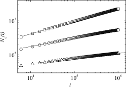
Figure 1: Log-log plots of the total number of product particles vs time for $\gamma=0.75$ (squares), $\gamma=0.5$ (circles), and $\gamma=0.25$ (triangles). The linear fit slopes are $0.37$, $0.25$, and $0.15$ respectively. The mean field prediction for the slope is given in Eq. (28) as $\gamma/2$.

Figure 1 shows our simulation results for the total number of product particles as a function of time in units of $\tau=1.0$ (used throughout) for several values of $\gamma$. This is perhaps the most robust global quantity to be simulated. The linear fit slope is given for each $\gamma$, and agrees very well with the theoretical prediction given in Eq. (26) for the two larger values of $\gamma$.

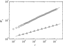
Figure 2: Width $W_{d}$ of the depletion zone vs time for $\gamma=0.5$ (circles) and $\gamma=0.25$ (triangles). The linear fit slopes are $0.257$ and $0.154$ respectively. The mean field prediction for the slope is given in Eq. (28) as $\gamma/2$.

Figure 2 shows our simulation results for the width of the depletion zone as a function for time for two values of $\gamma$. The linear fit slope is in good agreement with the theory as given in Eq. (28) for the larger value of $\gamma$. Later we discuss some difficulties, particularly for small values of $\gamma$, in the accurate simulation of the profile $U_{P}(x,t)$ whose width is used to obtain these results.

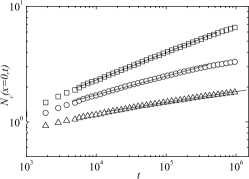
Figure 3: Log-log plots of the production profile of product $C$ at $x=0$ as a function of time for $\gamma=0.75$ (squares), $\gamma=0.5$ (circles), and $\gamma=0.25$ (triangles). The linear fit slopes are $0.24$, $0.162$, and $0.093$ respectively. The mean field prediction for the slope is given in Eq. (29) as $\gamma/3$.

Figure 3 shows our simulation results for the production profile of the product of the reaction at $x=0$ as a function of time, for several values of $\gamma$. For the larger $\gamma$ the linear fit slope agrees well with the theoretical prediction given in Eq. (29).

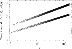
Figure 4: Time integrals of reactant concentrations at the center of the reaction zone. The mean field prediction for the slopes is given in Eq. (30) as $1-\gamma/3$. The steeper curve is for $\gamma=0.25$ and the reaction events governed by the exponential distribution Eq (33) with $\kappa=10^{-5}$. The linear fit slope is $0.814$ while mean field theory yields $0.917$. The shallower curve is for $\gamma=0.5$ and $\kappa=10^{-4}$. The linear fit slope is $0.683$, the mean field slope is $0.833$.

Figure 4 presents our simulation results for the time-integral of the concentration of a reactant at the center of the reaction zone, to be compared with the theoretical prediction of Eq. (30). While the agreement is not spectacular, the trend is correct. Also of interest here is the improved agreement when the reaction rate is greatly reduced, as expected. Even more dramatic effects of the reaction rate are seen below in the context of our discussion of the profile $U_{P}(x,t)$.

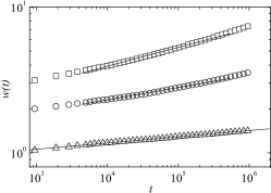
Figure 5: Log-log plot of the width of the product profile as a function of time for $\gamma=0.75$ (squares), $\gamma=0.5$ (circles), and $\gamma=0.25$ (triangles). The linear fit slopes are $0.129$, $0.084$, and $0.042$ respectively. The mean field prediction for the slope is given in Eq. (31) as $\gamma/6$.

Figure 5 contains our simulation results for the width of the product profile, which should be compared with the prediction of Eq. (31). The agreement is very good for all the values of $\gamma$.

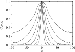
Figure 6: Simulation results for the profile $U_{P}(x,t)$ for $\gamma=0.75$ and $t=946$, $3777$, $15073$, $60149$, $240025$, and $957828$. The width of the profiles increase with time, as seen in Fig. 5. The simulation was carried out on a lattice of size $(160,20)$ and averaged over $102$ runs. Notice the apparent evolution from a characteristic sharp-pointed profile for short times to a vaulted profile at longer times. For a discussion of this anomaly, and for the values of other parameters, see text.

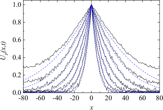
Figure 7: Simulation (jagged lines) and theory (dashed lines) for the profile $U_{P}(x,t)$ for $\gamma=0.75$ and $t=3738$, $8577$, $19682$, $45165$, $103638$, $237815$, and $545708$. Notice the absence of the rounding anomalies in the profile for small $x$. The reaction rate is much smaller in this case, see text. The simulation was carried out on a lattice of size $(160,20)$ and averaged over $102$ runs. The times are approximately equivalent to those used in Fig. 6 if the total number of $C$ particles in the system is used as a measure of time.

Finally, in Figs. 6 and 7 we present perhaps the most difficult quantity to capture accurately, namely, the profile $U_{p}(x,t)$ defined in Eq. (27). For these simulations we use a lattice of size $(L_{x},L_{y})=(160,20)$. As pointed out earlier, the difficulty arises from the fact that it involves regions of very low concentration. It is instructive to illustrate the difficulty, and that is why we have included Fig. 6. The simulation profiles shown at the different times are actually time averaged over a small time interval around the times shown. The noteworthy feature is the evolution of the sharp-pointed profile near the origin at short times to a more rounded shape at longer times. The mean field theory presented in this paper does not produce this rounding, so that it seemed at first that the theory and simulations differed in some profound way. However, the simulations in Fig. 6 were carried out with the rate coefficient $k=0.05$ with reactions occurring periodically at time interval $\Delta t_{r}=10$, a reaction rate that turns out to be too high for comparison with our theory. In Fig. 7 we show both the simulation results (jagged curves) and those of our theory (dashed curves), now with exponentially distributed reaction events according to Eq. (33), with $\kappa=10^{-5}$. The profile near $x=0$ remains pointed for all the times shown, as predicted by the theory. The quantitative disagreements for long times ($t=237185$ and especially $t=545708$) are due to finite size effects. Boundary effects are negligible only as long as $U_{p}(x=-L_{x}/2,t)=U_{P}(x=L_{x}/2,t)=0$, and for the long times we find that this is not the case. In our other simulation results we have not included such results in our averages, but have left them in this figure simply to stress the finite size effects one must be aware of in calculating the behavior of quantities in the depletion zone when the zone extends all the way to the boundaries of the system. To provide accurate results for such long times it is necessary to run simulations on larger systems.

V Closing Comments

In this paper we have proposed a set of continuum fractional diffusion equations to describe the behavior of a reaction front in the $A+B\to C$ reaction-subdiffusion problem. Subdiffusion may be appropriate to describe the way reactants move in complex (glassy, disordered, highly constrained) geometries, and we were interested in exploring how this constraint on the motion would affect the evolution of a reaction front. Because we are working with a set of mean field continuum equations, our results are only valid above the critical dimension $d=2$.

The subdiffusive motion is modeled via the usual fractional equation that contains the Riemann-Liouville operator, Eq. (5). This choice has a long history, and its virtues and shortcomings are clearly understood. Less clear has been the selection of the local reaction term, and the question of the way in which the memory in the Riemann-Liouville operator does (or does not) affect the way in which the reaction is modeled. While the literature on this subject has presented a number of viewpoints, we argued, in agreement with seki1 ; seki2 , that the reaction term should also be modified from its usual simple instantaneous product form, at least for small reaction rate constants. Our reaction-subdiffusion model is thus given by Eq. (23).

Following the approach of Gálfi and Rácz galfi for the evolution of a front in the reaction-diffusion problem, we assumed scaling solutions for the various quantities that can be calculated from the model. Some of these quantities depend explicitly on the form chosen for the reaction term while others do not. We compared the resulting exponents with those obtained from numerical simulations. We found very good agreement between the theory and simulations for the exponents $\mu$ and $\alpha$ that characterize the reaction term, Eq. (7). In particular, in terms of the power $\gamma<1$ that characterizes the subdiffusive process we found that the theoretical values $\mu=1-\gamma/3$ and $\alpha=\gamma/6$ are recovered in the simulations with greater fidelity for larger $\gamma$. The exponent $\theta$, governing the time decay of the reactant concentrations as in Eq. (6), is, theoretically, given by $\gamma/3$. Simulation results give values which correctly follow this trend, but the agreement is not quantitative. However, we have to remember that the quantity $a(0,t)$ is local and, consequently, it is more difficult to achieve good statistical averages with the small systems and number of particles considered in the simulations. Perhaps the most challenging quantity to capture is the profile $U_{P}(x,t)$. The theory predicts a cusp at $x=0$ which we were able to capture by our simulations when the reaction rate constant is sufficiently small. The quantitative agreement between the theory and the simulations for this profile was ultimately limited by our finite system size. We note that our results are a good example of what is sometimes referred to as subordination in that the subdiffusive scaling behavior can be deduced from the corresponding diffusive behavior with the substitution $t\to t^{\gamma}$ subordination .

This work can clearly be pursued along a number of directions. Among them is the description of this same reaction-subdiffusion problem with the usual uniform initial condition for the species, to investigate what sorts of segregation patterns might evolve on the way to extinction, or on the way to equilibration if the reaction is reversible. Another is the study of the fluctuations that must be added to the model in order to describe this process in a one-dimensional system where the mean field description is no longer appropriate, and the possible logarithmic correction in two dimensions that may explain some of our small-$\gamma$ discrepancies. A third is the effect of different subdiffusion coefficients for the species $A$ and $B$, and even of different exponents $\gamma_{A}$ and $\gamma_{B}$. In this latter case subordination would necessarily be more complicated if valid at all. Work along these directions is in progress newones .

- (1) For a review see E. Kotomin and V. Kuzovkov, Modern Aspects of Diffusion-Controlled Reactions: Cooperative Phenomena in Bimolecular Processes (Elsevier, Amsterdam, 1996).
- (2) D. C. Torney and H. McConnell, J. Phys. Chem. 87, 1941 (1983).
- (3) J. L. Spouge, Phys. Rev. Lett. 60, 871 (1988).
- (4) C. R. Doering and D. ben-Avraham, Phys. Rev. A 38, 3035 (1988); M. A. Burschka, C. R. Doering and D. ben-Avraham, Phys. Rev. Lett. 63, 700 (1989); D. ben-Avraham, M. A. Burschka and C. R. Doering, J. Stat. Phys. 60, 695 (1990); D. ben-Avraham, Mod. Phys. Lett. 9, 895 (1995).
- (5) K. Lindenberg, P. Argyrakis and R. Kopelman, J. Phys. Chem. 99, 7542 (1995).
- (6) K. Krebs, M. P. Pfannmuller, B. Wehefritz and H. Hinrichsen, J. Stat. Phys 78, 1429 (1995).
- (7) T. O. Masser and D. ben-Avraham, Phys. Lett. A 275, 382 (2000); Phys. Rev. E 63, 066108 (2001); Phys. Rev. E 64, 062101 (2001).
- (8) S. Habib, K. Lindenberg, G. Lythe and C. Molina-París, J. Chem. Phys. 115, 73 (2001).
- (9) C. Mandache and D. ben-Avraham, J. Chem. Phys. 112, 7735 (2000).
- (10) M. Henkel and H. Hinrichsen, J. Phys. A 34, 1561 (2001).
- (11) E. Abad, H. L. Frisch and G. Nicolis, J. Stat. Phys. 99, 1397 (2000).
- (12) A. A. Ovchinnikov and Y. G. Zeldovich, Chem. Phys 28, 215 (1978).
- (13) D. Toussaint and F. Wilczek, J. Chem. Phys. 78, 2642 (1983).
- (14) K. Kang and S. Redner, Phys. Rev. Lett. 52, 955 (1984).
- (15) R. Kopelman, Science 241, 1620 (1988) and references therein.
- (16) S. Kanno, Prog. Theor. Phys. 79, 721 (1988); ibid, 1330.
- (17) E. Clément, L. M. Sander, and R. Kopelman, Phys. Rev. A 39, 6455 (1989); ibid, 6466; ibid, 6472.
- (18) P. Argyrakis and R. Kopelman, Phys. Rev. A 41, 2114 (1990); ibid, 2121.
- (19) K. Lindenberg, B. J. West, and R. Kopelman, Phys. Rev. Lett. 60, 1777 (1988); ibid, Phys. Rev. A 42, 890 (1990); W-S. Sheu, K. Lindenberg, and R. Kopelman, Phys. Rev. A 42, 2279 (1990).
- (20) M. Bramson and J. L. Lebowitz, J. Stat. Phys. 62, 297 (1991).
- (21) F. Leyvraz and S. Redner, Phys. Rev. Lett. 66, 2168 (1991).
- (22) G. Zumofen, J. Klafter, and A. Blumen, Phys. Rev. A 45, 8977 (1992).
- (23) P. Argyrakis, R. Kopelman, and K. Lindenberg, Chem. Phys. 177, 693 (1993); K. Lindenberg, P. Argyrakis, and R. Kopelman, J. Phys. Chem. 98, 3389 (1994).
- (24) H. Taitelbaum, Y-E. L. Koo, S. Havlin, R. Kopelman, and G. H. Weiss, Phys. Rev. A 46, 2151 (1992); H. Taitelbaum, A. Yen, R. Kopelman, S. Havlin, and G. H. Weiss, Phys. Rev. E 54, 5942 (1996); H. Taitelbaum, B. Vilensky, A. Lin, A. Yen, Y-E. Lee Koo, and R. Kopelman, Phys. Rev. Lett. 77, 1640 (1996)
- (25) S. H. Park, S. Parus, R. Kopelman, and H. Taitelbaum, Phys. Rev. E 64, 055102(R) (2001).
- (26) C. N. Baroud, F. Okkels, L. Ménétrier, and P. Tabeling, Phys. Rev. E 67, 060104(R) (2003).
- (27) R. Kopelman, Z-Y. Shi, and C-S. Li, J. Lumin. 48/49, 143 (1991) and references therein.
- (28) S. Habib and G. Lythe, Phys. Rev. Lett. 84, 1070 (2000).
- (29) L. Gálfi and Z. Rácz, Phys. Rev A (Rapid Comm.) 38, 315 (1988).
- (30) Z. Jiang and C. Ebner, Phys. Rev. A 42, 7483 (1990).
- (31) S. J. Cornell, M. Droz, and B. Chopard, Phys. Rev. A 44, 4826 (1991).
- (32) S. J. Cornell, Phys. Rev. Lett. 75, 2250 (1995); S. J. Cornell, Phys. Rev. E 51, 4055 (1995).
- (33) E. ben-Naim and S. Redner, J. Phys. A 25, L575 (1992).
- (34) H. Larralde, M. Araujo, S. Havlin, and H. E. Stanley, Phys. Rev A 46, 855 (1992); H. Larralde, M Araujo, S. Havlin, and H. E. Stanley, Phys. Rev. A 46, R6121 (1992); M. Araujo, S. Havlin, H. Larralde, and H. E. Stanley, Phys. Rev. Lett. 68, 1791 (1992); M. Araujo, H. Larralde, S. Havlin, and H. E. Stanley, Phys. Rev. Lett. 71, 3592 (1993); M. Araujo, H. Larralde, S. Havlin, and H. E. Stanley, Phys. Rev. Lett. 75, 2251 (1995).
- (35) B. Chopard, M. Droz, T. Karapiperis, and Z. Racz, Phys. Rev. E 47, pR40 (1993); B. Chopard, D. Droz, J. Magnin, and Z. Racz, Phys. Rev. E 56 5343 (1997).
- (36) B. P. Lee and J. Cardy, Phys. Rev. E 50, R3287 (1994); G. T. Barkema, M. J. Howard, and J. L. Cardy, Phys. Rev. E 53, R2017 (1996).
- (37) P. L. Krapivsky, Phys. Rev. E 51, 4774 (1995).
- (38) Z. Koza, J. Stat. Phys. 85, 179 (1996); Z. Koza and H. Taitelbaum, Phys. Rev. E 54, R1040 (1996); Z. Koza and H. Taitelbaum, Phys. Rev. E 56, 6387 (1997); Physica A 240, 622 (1997); Philos. Mag. B 77, 1437 (1998); H. Taitelbaum and Z. Koza, Physica A 285, 166 (2000); Phys. Rev. E 66, 011103 (2002); Europhys. J. B 32, 507 (2003).
- (39) See e.g. R. Metzler and J. Klafter, Phys. Rep. 339, 1 (2000); B. J. West, M. Bologna, and P. Grigolini, Physics of Fractal Operators (Springer, New York, 2003).
- (40) D. ben-Avraham and S. Havlin, Diffusion and Reactions in Fractals and Disordered Systems (Cambridge University Press, Cambridge, 2000);
- (41) T. Kostołowicz, K. Dworecki, and St. Mrówczyński, cond-mat/0309072.
- (42) S. B. Yuste and K. Lindenberg, Phys. Rev. Lett. 87, 118301 (2001); ibid, Chem. Phys. 284, 169 (2002).
- (43) J-C. Lin, C. R. Doering and D. ben-Avraham, Chem. Phys. 146, 355 (1990); J-C. Lin, Phys. Rev. A 44, 6706 (1991).
- (44) For reviews see J. W. Haus and K. Kehr, Phys. Rev. 150, 264 (1987); J.-P. Bouchaud and A. Georges, Phys. Rep. 195, 127 (1990).
- (45) E. Barkai, Chem. Phys. 284, 13 (2002).
- (46) I. M. Sokolov, A. Blumen and J. Klafter, Europhys. Lett. 56, 175 (2001).
- (47) R. Hilfer, Editor, Applications of Fractional Calculus in Physics, (World Scientific, Singapore, 2000); V. Balakrishnan, Physica A 132, 569 (1985); C. R. Doering and D. ben-Avraham, Phys. Rev. Lett. 62, 2563 (1989); R. Metzler, E. Barkai and J. Klafter, Phys. Rev. Lett. 82, 3563 (1999);
- (48) R. Metzler, E. Barkai and J. Klafter, Europhys. Lett. 46, 431 (1999); E. Barkai, R. Metzler, and J. Klafter, Phys. Rev. E 61, 132 (2000).
- (49) W. R. Schneider and W. Wyss, J. Math. Phys. 30, 134 (1989).
- (50) A. M. Mathai and R. K. Saxena, The H-function with Applications in Statistics and Other Disciplines, (John Wiley and Sons, New York,1978).
- (51) D. ben-Avraham, Mod. Phys. Lett. 9, 895 (1995).
- (52) B. I. Henry and S. L. Wearne, Physica A 276, 448 (2000); B. I. Henry and S. L. Wearne, SIAM (Soc. Ind. Appl. Math.) J. Appl. Math. 62, 870 (2002); M. O. Vlad and J. Ross, Phys. Rev. E 66, 061908 (2002); S. Fedotov and V. Méndez, Phys. Rev. E 66, 030102 (20020).
- (53) J. Sung, E. Barkai, R. J. Silbey, and S. Lee, J. Chem. Phys. 116, 2338 (2002).
- (54) K. Seki, M. Wojcik, and M. Tachiya, J. Chem. Phys. 119, 2165 (2003).
- (55) K. Seki, M. Wojcik, and M. Tachiya, J. Chem. Phys. 119, 7525 (2003).
- (56) D. R. Cox and H. D. Miller, The Theory of Stochastic Processes (Wiley, New York, 1965).
- (57) D. Bedeaux, K. Lakatos-Lindenberg, and K. E. Shuler, J. Math. Phys. 12, 2116 (1971).
- (58) V. M. Kenkre, E. W. Montroll, and M. F. Shlesinger, J. Stat. Phys. 9, 45 (1973).
- (59) A. Blumen, J. Klafter, and G. Zumofen, in Optical Spectroscopy of Glasses, ed. I. Zschokke (Reidel, Dordrecht, 1986); A. Blumen, J. Klafter, B. S. White, and G. Zumofen, Phys. Rev. Lett. 53, 1301 (1984); J. Klafter, A. Blumen, and G. Zumofen, J. Stat. Phys. 36, 561 (1984).
- (60) S. B. Yuste et al., in preparation.