Statistics of Transmission Eigenvalues for a Disordered Quantum Point Contact

Abstract

We study the distribution of transmission eigenvalues of a quantum point contact with nearby impurities. In the semi-classical case (the chemical potential lies at the conductance plateau) we find that the transmission properties of this system are obtained from the ensemble of Gaussian random reflection matrices. The distribution only depends on the number of open transport channels and the average reflection eigenvalue and crosses over from the Poissonian for one open channel to the form predicted by the circuit theory in the limit of large number of open channels.

I Introduction

A quantum point contact (QPC) is one of the reference systems of mesoscopic physics. The experimental discovery of conductance quantizaton Expqpc triggered further research which contributed much to our modern understanding of nanoscience. QPC is a constriction defined in a 2DEG by gates. The width of the constriction can be changed by the voltage applied to these gates. In the adiabatic regime, if the distance between the gates changes slowly compared to the wavelength of an electron, the theoretical description is readily obtained Glazman ; Buttiker . The two-dimensional motion of an electron confined between the gates is equivalent to one-dimensional scattering of an electron at a potential barrier. The height of the barrier is different for different transport channels. Semi-classically, the electron is fully transmitted if its energy exceeds the top of the barrier in a given channel, and is fully reflected otherwise. Thus, semi-classical transmission eigenvalues of a QPC are strongly degenerate: One has a finite number of transmission eigenvalues equal to one and an infinite number of transmission eigenvalues equal to zero. This picture would manifest experimentally in the precise quantization of conductance as a function of gate voltage.

In real experiments, this degeneracy is lifted. A brief glance at any of many available experimental studies shows that conductance does not rise in ideal steps. The question whether the transmission eigenvalues are degenerate is also important for a number of other reasons. For instance, if a QPC is prepared in a superconducting material, discrete subgap (Andreev) states develop Andreev . These states describe quasiparticles localized around QPC. The number of these states equals the number of transport channels, and their energies are expressed via transmission eigenvalues $T_{n}$, $E_{n}=\Delta\sqrt{1-T_{n}\sin^{2}\varphi/2}$, with $\Delta$ and $\varphi$ being the superconducting gap and the phase difference across the QPC. If the transmission eigenvalues are degenerate, the Andreev levels are also degenerate. Thus, any small perturbation would lift this degeneracy and produce a number of states with very close energies. Such a perturbation would then drastically affect properties of the system.

An obvious candidate for this degeneracy lifting is quantum tunneling across the top of the barrier. Indeed, for a given energy there is a range of gate voltages when one transport channel has a transmission eigenvalue between zero and one – a partially open channel. All other transmission eigenvalues are also modified by the quantum tunneling: They get an exponentially small correction. Thus, quantum tunneling leads to the rounding of the conductance steps as a function of gate voltage, but only provides exponentially small splitting of Andreev states.

In this paper, we study how the degeneracy of transmission eigenvalues is lifted by the scattering on impurities, which are always present in and around the QPC. Properties of a disordered QPC have been investigated (see Refs. Imry, ; Nixon, ; Glazman2, ; Maslov, ; Beenakker, ), mostly in relation to the disorder smearing of conductance steps or evolution of conductance fluctuations in ballistic regime. In contrast to the previous literature, we investigate the case when the conductance of the QPC is only slightly modified by the impurities, or, in other words, the impurity-related splitting of transmission eigenvalues is much less than one. This regime is realized for low concentration of impurities. In this situation we can disregard quantum effects like resonant tunneling through impurity states or Kondo effect.

Our main result is that in this regime, reflection amplitudes are Gaussian distributed with zero average and second-order correlation function which does not depend on the channel index. This provides us with a new class of random matrix theory. The results for the distribution function of transmission eigenvalues are universal — they only depend on the number of transport channels and on the average reflection eigenvalue. All other information can be extracted from these two parameters.

The paper is organized in the following way. In Section II we treat a disordered QPC in the adiabatic approximation. In Section III we introduce the scattering matrix and show that in the expansion up to the second order in disorder potential closed channels do not contribute to the properties of transmission eigenvalues of open channels. Section IV finalizes the quantum-mechanical calculation of reflection coefficient and conductance of a disordered QPC. We then turn to the classical (Boltzmann equation) consideration, which facilitates the consideration of the diffusive regime (Section V).

In Section VI we discuss noise properties of disordered QPC. Finally, Section VII is devoted to the distribution function of transmission eigenvalues. For one open transport channel, we calculate this distribution function analytically by performing the disorder averaging directly. In the limit of large number of open channels, we obtain the distribution function by means of the circuit theory Nazarov , which presents a disordered QPC as a pure QPC and a diffusive resistor connected in series. For intermediate numbers of open channels, we perform a numerical simulation based on random matrix theory.

II Model of QPC with impurities

We describe the QPC as a constriction between two infinitely high walls Glazman separated by the distance $d(x)$ (Figure 1). A more physical model would take into account that the transverse profile is not sharp Buttiker . Since in this paper we employ semi-classical approximation (do not discuss the rounding of conduction steps), the results do not depend on the details of the potential profile. For this reason, we use the simpler model. The Schrödinger equation,

$$\left[-\frac{\hbar^{2}}{2m}\nabla^{2}+V(x,y)\right]\psi(x,y)=E\psi(x,y),$$ (1)

is supplemented by the boundary conditions,

$$\psi(x,y={\pm}d(x)/2)=0.$$

Here

$$V(x,y)=\sum_{i}\,v(x-x_{i},y-y_{i}),$$

with $v$ being the single impurity potential, and the sum is taken over impurity positions.

If the width of the constriction $d(x)$ changes smoothly, we can employ the adiabatic approximation and separate the transverse motion,

$$\psi(x,y)=\sum_{n}\phi_{n}(x)\varphi_{n}^{(x)}(y).$$

The transverse wave functions $\varphi_{n}^{(x)}(y)$ that satisfy the boundary conditions are

$$\varphi_{n}^{(x)}(y)=\sqrt{\frac{2}{d(x)}}\sin\left[\frac{n\pi}{d(x)}\,\left(y+\frac{d(x)}{2}\right)\right].$$

Substituting this into Eq. (1) and disregarding the terms containing the derivatives of $d(x)$, we obtain a one-dimensional equation for the longitudinal wave function,

$$\left[-\frac{\hbar^{2}}{2m}\frac{d^{2}}{dx^{2}}+\epsilon_{n}(x)-E\right]\phi_{n}(x)=-\sum_{m}V_{nm}(x)\phi_{m}(x),$$ (2)

with the channel-dependent effective potential barrier

$$\epsilon_{n}(x)=\frac{\hbar^{2}\pi^{2}n^{2}}{2md^{2}(x)},$$

and the matrix element of the disorder potential,

$$V_{nm}(x)=\int_{-d(x)/2}^{d(x)/2}dy\,\varphi_{n}^{(x)}(y)V(x,y)\varphi_{m}^{(x)}(y).$$

Eq. (2) is the generalization of the equations previously written in Refs. Glazman, ; Buttiker, to the case of disordered QPC.

In the semi-classical (WKB) approximation, in the absence of disorder, for each transport channel, electrons with the energies above (below) the top of the barrier are perfectly transmitted (reflected). This approximation breaks down if the energy of an electron coincides with the top of the barrier. In this paper, we do not consider this case. The wave function of an ideally transmitted electron is

$$\phi_{n}^{(0)}(x)=\sqrt{\frac{p_{n}(\infty)}{p_{n}(x)}}\exp\left[\frac{i}{\hbar}\int^{x}p_{n}(z)dz\right],$$ (3)

with the channel-dependent momentum

$$p_{n}(x)=[2m(E-\epsilon_{n}(x))]^{1/2}.$$

III Correlators of the scattering matrix elements

We proceed by introducing the scattering matrix,

$$\hat{S}=\left(\begin{array}[]{cc}\hat{r}&\hat{t}\\ \hat{t}^{T}&\hat{r}^{\prime}\end{array}\right),$$

which is unitary, ${\hat{S}}^{\dagger}{\hat{S}}=1$, due to the current conservation requirement. At zero temperature, conductance of the system is expressed via Landauer formula,

$$G=G_{Q}\mbox{Tr}\,{\hat{t}}^{\dagger}{\hat{t}}=G_{Q}\sum_{n}T_{n},$$

where $T_{n}$ (of interest in this paper) are the eigenvalues of the matrix $\hat{t}^{\dagger}\hat{t}$, and $G_{Q}=e^{2}/\pi\hbar$ is the conductance quantum. Without impurities, the matrix $\hat{t}^{\dagger}\hat{t}$ is diagonal, with the elements describing the transmission of an electron in the same open transport channel equal one and all others equal zero. In this case, the conductance is $G_{0}=G_{Q}N$, with $N$ being the number of open transport channels.

To treat the effect of disorder, it is more convenient to investigate the matrix $\hat{r}^{\dagger}\hat{r}$, with the eigenvalues (reflection eigenvalues) $R_{n}=1-T_{n}$. In the following, we calculate the correction to the transmission eigenvalue $R_{n}$ due to disorder. For this purpose, we consider the perturbation expansion of the reflection matrix $\hat{r}$ up to the second order in the disorder potential,

$$\hat{r}=\hat{r}^{(0)}+\hat{r}^{(1)}+\hat{r}^{(2)}.$$

Let us now separate open and closed channels,

$$\hat{r}=\left(\begin{array}[]{cc}\hat{r}_{oo}&\hat{r}_{oc}\\ \hat{r}_{co}&\hat{r}_{cc}\end{array}\right),$$

where the submatrices $r_{\alpha\beta}$, $\alpha,\beta=o,c$ describe reflection from/to channels of different type ($o$ and $c$ stand for open and closed). The reflection eigenvalues are found from the secular equation, $\det\left({\hat{r}}^{\dagger}{\hat{r}}-R{\hat{1}}\right)=0$, or, equivalently,

$$\det\left(\begin{array}[]{cc}\hat{r}^{\dagger}_{oo}\hat{r}_{oo}+\hat{r}^{\dagger}_{co}\hat{r}_{co}-R{\hat{1}}&\hat{r}^{\dagger}_{oo}\hat{r}_{oc}+\hat{r}^{\dagger}_{co}\hat{r}_{cc}\\ \hat{r}^{\dagger}_{oc}\hat{r}_{oo}+\hat{r}^{\dagger}_{cc}\hat{r}_{co}&\hat{r}^{\dagger}_{oc}\hat{r}_{oc}+\hat{r}^{\dagger}_{cc}\hat{r}_{cc}-R{\hat{1}}\end{array}\right)=0.$$ (4)

We now expand this equation in powers of the disorder potential. For open channels, the reflection eigenvalues $R$ are expected to be of the second order in disorder. We use now the identity

$$\det\left(\begin{array}[]{cc}A&B\\ C&D\end{array}\right)=\det(A-BD^{-1}C)\det D,$$

and expand the first determinant taking into account that $\hat{r}^{(0)}_{oc}=\hat{r}^{(0)}_{co}=\hat{r}^{(0)}_{cc}=0$. The terms of zeroth order in the disorder potential cancel, since $\hat{r}^{(0){\dagger}}_{cc}\hat{r}^{(0)}_{cc}=1$. Terms of the first order do not appear, and in the second order one has $\det(\hat{r}^{(1){\dagger}}_{oo}r^{(1)}_{oo}-R{\hat{1}})=0$. Thus, closed channels have no effect on transmission of open channels. In the rest of the paper, we drop the subscript $oo$ and operate only with the quantities related to open channels.

Elements of the matrix $\hat{r}$ are random quantities. In the next Section, we characterize their statistical properties. We show that they are Gaussian distributed with zero average. Thus, it is enough to specify the correlation functions

$$\langle{\hat{r}}_{ij}^{*(1)}{\hat{r}}_{kh}^{(1)}\rangle,$$

where the average is performed with respect to disorder. We show that the only non-zero correlator is $\left\langle|r^{(1)}_{ij}|^{2}\right\rangle$, which is the probability for an electron coming in the open channel $i$ to be scattered to the open channel $j$. As a matter of fact, the result does not depend on the indices $i$ and $j$. We then relate this reflection probability with the correction to the conductance.

Thus, the set of eigenvalues $R_{n}$ describing open channels is obtained by diagonalizing the finite-size random matrix $\hat{r}^{{\dagger}}\hat{r}$. This matrix is Gaussian, and depends only on one parameter — average reflection coefficient. This novel random matrix theory in later Sections provides a novel distribution of transmission eigenvalues.

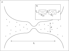
Figure 1: (a) Layout of a disordered QPC. (b) An equivalent circuit representing a disordered QPC as a clean QPC and a diffusive resistor in series.

IV Scattering matrix approach

To calculate the correction to the reflection amplitudes we consider the Green’s functions of Eq. (2),

$$\left[-\frac{\hbar^{2}}{2m}\frac{d^{2}}{dx^{2}}+\epsilon_{n}(x)-E\right]{\mathcal{G}}_{n}(x,x^{\prime})=-\delta(x-x^{\prime}).$$

Solving this equation, we find the Green’s functions for open channels,

$${\mathcal{G}}_{n}(x,x^{\prime})=\frac{i\hbar}{m\sqrt{p_{n}(x)p_{n}(x^{\prime})}}\exp\left[\frac{i}{\hbar}\left|\int_{x}^{x^{\prime}}dz\,p_{n}(z)\right|\right].$$ (5)

The formal solution of Eq. (2) takes the form

$$\phi_{n}(x)=\phi_{n}^{(0)}(x)+\int dx^{\prime}{\mathcal{G}}_{n}(x,x^{\prime})\sum_{m}V_{nm}(x^{\prime})\phi_{m}(x^{\prime}),$$ (6)

with $\phi_{n}^{(0)}$ being the solutions in the absence of disorder (Eq. (2) with the zero right-hand side.) In the first order in $V$, we obtain

$$\phi_{n}(x)=\phi_{n}^{(0)}(x)+\sum_{m}\int dx^{\prime}{\mathcal{G}}_{n}(x,x^{\prime})V_{nm}(x^{\prime})\phi^{(0)}_{m}(x^{\prime}).$$ (7)

Substituting Eqs. (3) and (5) into Eq. (7), we find

$$r_{nm} = \int_{-\infty}^{\infty}dx^{\prime}\frac{i\hbar}{m\sqrt{p_{n}(x^{\prime})p_{m}(x^{\prime})}}$$ (8)

$${\times} \exp\left[\frac{i}{\hbar}\int^{x^{\prime}}dz\left(p_{n}(z)+p_{m}(z)\right)\right]V_{nm}(x^{\prime}).$$

For the Gaussian distribution of disorder, the reflection amplitudes $r_{nm}$ are also Gaussian distributed. This distribution is fully characterized by the pair correlation function. If the impurities are not located in the constriction, the momenta $p_{n}(x)$ and $p_{m}(x)$ in Eq. (8) can be replaced by their values taken at $x\to\infty$, which is $p_{F}$ independently of the channel index. The impurity averaging is straightforward. As anticipated, all the averages of the type $\langle{\hat{r}}_{ij}^{*}{\hat{r}}_{kh}\rangle$ turn to zero due to the oscillating behavior, except for the term $\langle|r_{nm}|\rangle^{2}$,

$$\langle|r_{nm}|^{2}\rangle=\frac{n_{i}}{\hbar^{2}v_{F}^{2}}\frac{L}{d}\left|{\tilde{v}}(\pi)\right|^{2}\left(1+\frac{\delta_{nm}}{2}\right),$$ (9)

where ${\tilde{v}}(\pi)$ is the Fourier transform of the single impurity potential with the momentum transfer $2k_{F}$, and $n_{i}$ is the concentration of impurities per unit area.

The correction to the conductance reads

$$\langle\delta G\rangle=-G_{Q}\sum_{n,m=0}^{N}\langle|r_{nm}|^{2}\rangle,$$

and in the case of large number of open channels $N$ can be written as

$$\langle\delta G\rangle\simeq-\frac{e^{2}n_{i}}{\pi\hbar^{3}v_{F}^{2}}\frac{L}{d}|{\tilde{v}}(\pi)|^{2}N^{2}.$$ (10)

For further reference, we identify the average reflection eigenvalue $\langle R\rangle$ by means of Landauer formula, $\langle\delta G\rangle=-G_{Q}N\langle R\rangle$,

$$\langle R\rangle=\frac{n_{i}}{\hbar^{2}v_{F}^{2}}\frac{L}{d}|{\tilde{v}}(\pi)|^{2}N.$$

The correlation function of the reflection amplitudes can then be expressed via only one parameter $\langle R\rangle$,

$$\langle|r_{nm}|^{2}\rangle=\frac{1}{N}\left\langle R\right\rangle\left(1+\frac{\delta_{nm}}{2}\right).$$ (11)

V Boltzmann equation

In this Section we analyse transport properties of a disordered QPC in the framework of the Boltzmann equation. This approach allows for an extension of the analysis to the diffusive case, when the mean free path becomes much smaller then the length of the system. In this case the second order perturbation expansion breaks down, and the treatment of previous Sections can not be applied any more.

We model the system as a two-dimensional disordered wire between ideal reservoirs. To take into account the constriction, we recall that without disorder, in the quantum treatment only the channels with low index are ideally transmitting (open). In the language of classical physics, these channels correspond to electronic modes propagating with small incident angle $\alpha$ (Figure 2). To implement this feature in our model, we assume that all electrons propagating with angles smaller (larger) then $\alpha_{0}\ll 1$ are perfectly transmitted through the cross-section $x=0$ (to model the position of QPC). Electrons with higher angles are reflected from this cross-section. The Boltzmann equation reads

$${\bm{v}}{\cdot}{\bm{\nabla}_{r}}f({\bm{r}},{\bm{p}})=I[f],$$ (12)

where $f({\bm{r}},{\bm{p}})$ is the distribution function of electrons, and $I[f]$ is the collision integral abrikosov ,

$$I[f]=\frac{2\pi n_{i}}{\hbar}\int\frac{d^{2}{\bm{p}^{\prime}}}{(2\pi\hbar)^{2}}[f({\bm{r},\bm{p}}^{\prime})-f({\bm{r},\bm{p}})]$$

$${\times}|{\tilde{v}}({\bm{p}-\bm{p}^{\prime}})|^{2}\delta\left(\epsilon({\bm{p}}^{\prime})-\epsilon({\bm{p}})\right).$$

Since only electrons with energies betwen $E_{F}$ and $E_{F}+eV$, with $V$ being the applied voltage, contribute to the net current, the absolute value of the momentum $p$ is fixed to lie at the Fermi surface. We are only interested in the angular dependence of the distribution function, $f(x,\alpha)$. The Boltzmann equation (12) is supplemented by the boundary conditions,

$$\left\{\begin{array}[]{lr}f(x,\alpha)=1,&\cos\alpha>0,x<0\\ f(x,\alpha)=0,&\cos\alpha<0,x>L,\end{array}\right.$$

which state that electrons coming from the reservoirs are in thermal equilibrium. To take into account reflection of electrons at the QPC, we introduce the further boundary condition,

$$f(0,\alpha)=f(0,\pi-\alpha),\ \ \ \ \ |\cos\alpha|<\cos\alpha_{0}.$$

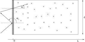
Figure 2: Disordered QPC modeled classically. Electrons with the angle $\alpha$ lower than the critical angle $\alpha_{0}$ are transmitted through the cross-section $x=0$, others are reflected from this cross-section.

The distribution function does not depend on the transverse coordinate $y$, and we thus rewrite Eq. (12) as

$$v_{F}\cos\alpha\ \partial_{x}f(x,\alpha)$$

$$= \frac{n_{i}m}{2\pi\hbar^{2}}\int d\alpha^{\prime}\cos\alpha^{\prime}\left|{\tilde{v}}(\alpha-\alpha^{\prime})\right|^{2}\left[f(x,\alpha)-f(x,\alpha^{\prime})\right].$$

We solve now Eq. (V) in the two limiting cases of low and high impurity concentration. The first case corresponds to the consideration of previous Sections based on the scattering approach. The second one, instead, allows us to investigate the diffusive regime.

V.1 Non-diffusive regime

For low impurity concentration, we replace the function $f(x,\alpha^{\prime})$ in the rhs of Eq. (V) with the distribution function of the pure system. The remaining differential equation is readily solved, yielding for the distribution function at $x=0$ and with the direction of propagation $|\cos\alpha|>\cos\alpha_{0}$,

$$f(0,\alpha)=\left\{\begin{array}[]{ll}1,&\cos\alpha>0\\ \displaystyle-\frac{\alpha_{0}Ln_{i}m|{\tilde{v}}(\alpha)|^{2}}{v_{F}\pi\hbar^{3}\cos\alpha},&\cos\alpha<0\end{array}\right..$$

Now we calculate the current density, ${\bm{j}}=(e\nu(E_{F})v_{F}/2\pi)\int d\alpha\cos\alpha f(0,\alpha)$, with $\nu(E_{F})$ being the density of states at the Fermi energy. Only the angles $|\cos\alpha|>\cos\alpha_{0}$ contribute, and we obtain the conductance,

$$G=e^{2}v_{F}\nu(E_{F})\left[2\alpha_{0}-2\alpha_{0}^{2}\frac{n_{i}m}{2\pi\hbar^{3}v_{F}}L|{\tilde{v}}(\pi)|^{2}\right]d,$$ (14)

where we have taken into account that $\alpha_{0}\ll 1$. The second term represents the correction to the conductance due to impurity scattering. Relating the number of open channels to the critical angle $\alpha_{0}$, $\alpha_{0}=2N\pi/k_{F}d$, we find that this correction is identical to Eq. (10), which we obtained from the scattering matrix approach in the limiting case $N\gg 1$.

V.2 Diffusive regime

For high impurity concentration, we introduce the transport relaxation time $\tau$, defined as abrikosov

$$\tau^{-1}=\frac{n_{i}m}{2\pi\hbar^{3}}\int_{0}^{2\pi}d\alpha|\tilde{v}(\alpha)|^{2}(1-\cos\alpha).$$

In the linear regime, the collision integral takes the form $I[f]=-(f-{\bar{f}})/\tau$, where $\bar{f}$ is the distribution function averaged over the angles,

$${\bar{f}}=\frac{1}{2\pi}\int_{0}^{2\pi}d\alpha f(\alpha).$$

Solution of the Boltzmann equation in this case is given by

$$f(x,\alpha)=\left(\frac{\pi l}{2L\alpha_{0}}+1\right)^{-1}\left(1-\frac{x}{L}+\frac{l}{L}\cos\alpha\right),$$

with $l=v_{F}\tau$ being the mean free path, $l\ll L$. Calculating the current, we find that the conductance is

$$G=\frac{e^{2}v_{F}\nu(E_{F})d}{2\pi}\left(\frac{1}{2\alpha_{0}}+\frac{L}{\pi l}\right)^{-1}.$$ (15)

Identifying the conductance of the diffusive region,

$$G_{D}=\frac{e^{2}v_{F}\nu(E_{F})ld}{2L},$$

and of the clean QPC,

$$G_{QPC}=\frac{e^{2}v_{F}\nu(E_{F})d}{2\pi}2\alpha_{0}=G_{Q}N,$$

we see that Eq. (15) represents a series addition of the conductances of the clean QPC and a diffusive resistor.

VI Noise

In a two-terminal system, zero-temperature shot noise BB can be expressed in terms of reflection eigenvalues in the following way,

$${\mathcal{S}}=\frac{e^{3}|V|}{\pi\hbar}\left\langle\sum_{n}R_{n}(1-R_{n})\right\rangle.$$

In a clean QPC, all transmission eigenvalues in the semi-classical regime are either zero or one, and the current is noiseless. Quantum tunneling away from the conductance steps only brings exponentially small contribution. Thus, we expect a drastic effect of disorder on the shot noise of a QPC. Indeed, up to the second order in the disorder potential, one writes

$${\mathcal{S}}=-\frac{2e^{3}|V|}{\pi\hbar}\sum_{n}\delta R_{n}=-2e|V|\delta G=2eG_{Q}N|V|\langle R\rangle.$$ (16)

Eq. (16) corresponds to the notion of Poissonian stream of reflected particles, which is, indeed, expected in the case of good transmission.

VII Distribution function

Now, we turn to the calculation of the distribution function of transmission eigenvalues,

$$\rho(T)=\left\langle\sum_{n}\delta(T-T_{n})\right\rangle,$$

where the sum is taken over all open channels, and disorder averaging is performed. The distribution function is normalized so that its integral is the number of open channels $N$. For a clean QPC, $\rho(T)=N\delta(1-T)$.

We first consider the case of one open channel and perform the disorder averaging directly. Then, we obtain analytical results in the limiting case of very large number of channels based on the circuit theory: A disordered QPC is presented as a clean QPC connected in series with a diffusive resistor. For intermediate values of $N$, we were not able to obtain analytical results. Instead, we perform a simulation based on the notion of random reflection matrices.

VII.1 One open channel

For one open channel, we perform a “brute force” disorder averaging. The reflection probability is $R=|r|^{2}$, where we have suppressed the channel indices. In its turn, the reflection amplitude $r$ is related to the potential $V$ by Eq. (8), with $m=n=1$. It is a complex quantity, and we first calculate the distribution function of the transmission amplitude, defined as

$${\mathcal{P}}(r)=\left\langle\delta\left(\mbox{Re}(r-r[V])\right)\delta\left(\mbox{Im}(r-r[V])\right)\right\rangle.$$

Representing delta-functions as integrals, we write explicitly

$${\mathcal{P}}(r)=\left\langle\int_{-\infty}^{\infty}\frac{d\omega_{1}d\omega_{2}}{(2\pi)^{2}}\right.$$ (17)

$$\times \left.\exp\left\{i\omega_{1}\mbox{Re}\left[r[V]-r\right]+i\omega_{2}\mbox{Im}\left[r[V]-r\right]\right\}\right\rangle.$$

Performing the averaging with the Gaussian distribution $\tilde{\mathcal{P}}[V]$, and introducing the short-hand notation

$$r[V]=\int d{\bm{r}}F({\bm{r}})V({\bm{r}}),$$

we obtain

$${\mathcal{P}}(r)=\int_{-\infty}^{\infty}\frac{d\omega_{1}d\omega_{2}}{(2\pi)^{2}}\exp\left\{-\frac{1}{2}\int d{\bm{r}_{1}}d{\bm{r}_{2}}\left[\omega_{1}\mbox{Re}F({\bm{r}_{1}})+\omega_{2}\mbox{Im}F({\bm{r}_{1}})\right]\left\langle V({\bm{r}_{1}})V({\bm{r}_{2}})\right\rangle\left[\omega_{1}\mbox{Re}F({\bm{r}_{2}})+\omega_{2}\mbox{Im}F({\bm{r}_{2}})\right]\right.$$

$$\left.-i\omega_{1}\mbox{Re}\,r-i\omega_{2}\mbox{Im}\,r\right\}.$$

Now we use Eq. (8) and disregard the terms containing rapidly oscillating functions. Calculating the integrals over $d\omega_{1}$ and $d\omega_{2}$, we finally obtain

$$\mathcal{P}(r)=\frac{1}{\pi\langle|r|^{2}\rangle}\exp\left(-\frac{|r|^{2}}{\langle|r|^{2}\rangle}\right).$$ (18)

Since $dR=2|r|d|r|=\pi^{-1}d\ {\mbox{R}e}r\ d\ \mbox{Im}r$, we can rewrite Eq. (18) in terms of the reflection eigenvalue,

$$\rho(R)=\frac{1}{\langle R\rangle}\exp\left(-\frac{R}{\langle R\rangle}\right);\ \ \ \rho(T)=\rho(1-R).$$ (19)

Thus, for one channel the reflection eigenvalue is Poisson distributed. This result is actually not surprising. Indeed, both real and imaginary parts of $r$ are linearly related to the potential $V$. This means they are both Gaussian with zero average. Moreover, from Eq. (8) it follows that they have the same dispersion, and we arrive to the Gaussian distribution for $r$ (18) and Poisson distribution for $R$ (19). These distributions are universal: All the information about the type and amplitude of disorder is encoded in only one number, which is the average reflection eigenvalue $\langle R\rangle$.

VII.2 Circuit Theory

If the number $N$ of open channels is large ($G\gg G_{Q}$), we can calculate the distribution function $\rho(T)$ analytically by means of the circuit theory developed by one of the authors Nazarov . To this purpose, we represent a disordered QPC as a clean QPC connected in series to a diffusive conductor (Figure 1). Such a point of view, to our knowledge, was first adopted in Ref. Maslov, for investigation of conductance fluctuations. The input parameters are the conductances of both circuit elements (connectors), $G_{QPC}$ and $G_{D}$. Each connector is subject to a phase difference $\phi$, which generates the pseudo-current $I(\phi)$. The relation $I(\phi)$ is determined by the distribution function of transmission eigenvalues,

$$\rho(T)\,=\,\frac{1}{2\pi G_{Q}}\frac{1}{T\sqrt{1-T}}\mbox{Re}\left[I\left(\pi+2i\mbox{arccosh}\frac{1}{\sqrt{T}}\right)\right].$$

In our case, the current-phase relations are

• Diffusive conductor: $I(\phi)=G_{D}\phi$

• Quantum point contact $I(\phi)=2G_{QPC}\tan(\phi/2)$

The circuit theory shows how these two elements can be combined to get the distribution function of the entire circuit. To this purpose, we introduce the phases: $\phi$ in the left reservoir; zero in the right reservoir, and $\theta$ (to be calculated) in the point (node) separating the QPC and diffusive conductor. Thus, the QPC is subject to the phase difference $\phi-\theta$, and the diffusive conductor to the phase difference $\theta$. The pseudo-current must be conserved, from which we get the following equation for $\theta$,

$$G_{D}\theta=2G_{QPC}\tan((\phi-\theta)/2).$$ (20)

After solving this equation, we find the pseudo-current $I(\phi)=G_{D}\theta(\phi)$, and eventually the distribution function.

Eq. (20) can not be solved analytically for an arbitrary relation between $G_{D}$ and $G_{QPC}$, and we restrict ourselves to the case of low impurity concentration, $G_{D}\gg G_{QPC}$. We obtain

$$I(\phi)\,=\,G_{D}\left[\frac{\phi-\pi}{2}+\sqrt{\frac{(\phi-\pi)^{2}}{4}+\frac{4G_{QPC}}{G_{D}}}\right],$$

and the distribution function follows,

$$\rho(T)=\frac{G_{D}}{2\pi G_{Q}}\frac{1}{T\sqrt{1-T}}\sqrt{T-T_{c}},$$ (21)

for $T>T_{c}$, $T_{c}=1-4G_{QPC}/G_{D}$, and zero for $T<T_{c}$. For further comparison with the simulation results, we calculate the average reflection coefficient $\langle R\rangle=G_{QPC}/G_{D}\ll 1$ and rewrite the distribution function (21) as

$$\rho(R)=\frac{N}{2\pi\langle R\rangle}\frac{1}{1-R}\sqrt{\frac{4\langle R\rangle}{R}-1}.$$ (22)

We see that in the limiting case $N\gg 1$ only channels with the transmission close to perfect exist: Reflection eigenvalues can only be lower than $4\langle R\rangle$, which is a small number. This is in contrast to the one-channel case, where all values of the reflection coefficient are permitted. To demonstrate the crossover between these two limiting cases, we perform a numerical simulation for the intermediate number of open transport channels.

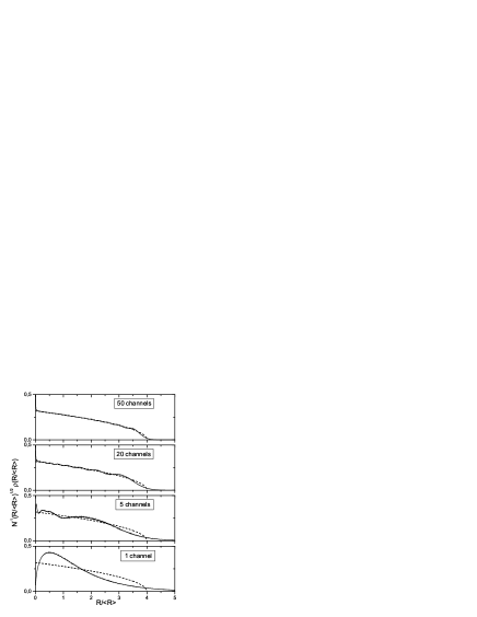
Figure 3: The distribution function of reflection eigenvalues $\rho(R)$ for 1, 5, 20 and 50 open channels. It is calculated using an ensamble of $10^{6}$ random matrices. The dashed line is the expression (22) valid in the limit $N\rightarrow\infty$.

VII.3 Intermediate case

For any number of open channels, the matrix elements of the reflection matrix, $r_{nm}$ are random quantities with Gaussian distribution. They are zero on average, uncorrelated, and characterized by the dispersion $\langle|r_{nm}|^{2}\rangle$. Eq. (9) shows that this dispersion is with the factor of $3/2$ greater for diagonal elements that for non-diagonal elements, and otherwise does not depend on $n$ and $m$. Then, the problem has only two parameters — the number of open transport channels $N$, and the dispersion of matrix elements of the reflection matrix. The latter parameter is related to the average reflection eigenvalue.

Thus, we model the reflection matrix as a Gaussian random matrix with independent elements $r_{nm}$. Both real and imaginary part of $r_{nm}$ are taken to be Gaussian distributed with the same dispersion (independent on $n$ and $m$). The simulation involves $10^{6}$ matrices. Results for $1$, $5$, $20$, and $50$ channels are plotted in Figure 3. For better comparison with Eq. (22), we multiply the distribution function with $R^{1/2}$, so that it tends to a constant value at $R\to 0$. For one channel, the simulation result perfectly reproduces the Poisson distribution (19), whereas for $50$ channels it is in a good agreement with Eq. (22). For $5$ and $20$ channels, the simulations reveal an intermediate picture, with a tail at large $R$. Oscillations in the distribution function, pronounced for $5$, $20$, and $50$ channels, are related to the Wigner-Dyson correlations of eigenvalues of Gaussian random matrices.

VIII Conclusions

The main result of our paper is the distribution function of reflection eigenvalues of a disordered QPC. We have shown that for one open channel, one obtains Poisson distribution, and in the limit of infinitely many channels only very small reflection eigenvalues are allowed. We also performed numerical simulations for the intermediate regime. In all the cases, the results are universal in the sense that they only depend on the number of open transport channels and on the average reflection coefficient $\langle R\rangle$. To calculate $\langle R\rangle$, we developed a quantum-mechanical theory, and a classical calculation based on the Boltzmann equation. For low impurity concentration, classical and quantum-mechanical results are identical; additionally, classically one can treat the diffusive regime, to find that the conductance of a disordered QPC is given as a series resistance addition. We stress that although the results for $\langle R\rangle$ are model dependent, as carefully investigated previously by Glazman and Jonson Glazman2 , the form of the distribution function only uses $\langle R\rangle$ as a parameter, but does not depend on specific model any more. It can be regarded as a result of the novel random matrix theory with Gaussian reflection matrices.

This work was supported by the Netherlands Foundation for Fundamental Research on Matter (FOM).

References

- (1) B. J. van Wees, H. van Houten, C. W. J. Beenakker, J. G. Williamson, L. P. Kouwenhoven, D. van der Marel, and C. T. Foxon, Phys. Rev. Lett. 60, 848 (1988); D. A. Wharam, T. J. Thornton, R. Newbury, M. Pepper, H. Ahmed, J. E. F. Frost, D. G. Hasko, D. C. Peacock, D. A. Ritchie, and G. A. C. Jones, J. Phys. C 21, L209 (1988).
- (2) L. I. Glazman, G. B. Lesovik, D. E. Khmel’nitskii, and R. I. Shekhter, Pis’ma Zh. Éksp. Teor. Fiz. 48, 218 (1988) [JETP Lett. 48, 238 (1988)].
- (3) M. Büttiker, Phys. Rev. B 41, 7906 (1990).
- (4) A. Furusaki and M. Tsukada, Physica B 165 & 166, 967 (1990); C. W. J. Beenakker, Phys. Rev. Lett. 67, 3836 (1991).
- (5) I. Kander, Y. Imry, and U. Sivan, Phys. Rev. B 41, 12941 (1990).
- (6) J. A. Nixon, J. H. Davies, and H. U. Baranger, Phys. Rev. B 43, 12638 (1991).
- (7) L. I. Glazman and M. Jonson, Phys. Rev. B 44, 3810 (1991).
- (8) D. L. Maslov, C. Barnes, and G. Kirczenow, Phys. Rev. Lett. 70, 1984 (1993); Phys. Rev. B 48, 2543 (1993).
- (9) C. W. J. Beenakker and J. A. Melsen, Phys. Rev. B 50, 2450 (1991); C. W. J. Beenakker, Rev. Mod. Phys. 69 731 (1997).
- (10) Yu. V. Nazarov, in: Quantum Dynamics of Submicron Structures, ed. by H. A. Cerdeira, B. Kramer, and G. Schön, Kluwer Academic Publishers, Dordrecht (1995), p.687.
- (11) A. A. Abrikosov, Fundamentals of the Theory of Metals, North-Holland, Amsterdam (1988).
- (12) For review, see Ya. M. Blanter and M. Büttiker, Phys. Rep. 336, 1 (2000).