The Social Architecture of Capitalism

Abstract

A dynamic model of the social relations between workers and capitalists is introduced. The model is deduced from the assumption that the law of value is an organising principle of modern economies. The model self-organises into a dynamic equilibrium with statistical properties that are in close qualitative and in many cases quantitative agreement with a broad range of known empirical distributions of developed capitalism, including the power-law distribution of firm size, the Laplace distribution of firm and GDP growth, the lognormal distribution of firm demises, the exponential distribution of the duration of recessions, the lognormal-Pareto distribution of income, and the gamma-like distribution of the rate-of-profit of firms. Normally these distributions are studied in isolation, but this model unifies and connects them within a single causal framework. In addition, the model generates business cycle phenomena, including fluctuating wage and profit shares in national income about values consistent with empirical studies. A testable consequence of the model is a conjecture that the rate-of-profit distribution is consistent with a parameter-mix of a ratio of normal variates with means and variances that depend on a firm size parameter that is distributed according to a power-law.

url]ianusa.home.mindspring.com

Version 1 December 2003
Version 2 January 2004

1 Introduction

The dominant social relation of production within capitalism is that between capitalists and workers. A small class of capitalists employ a large class of workers organized within firms of various sizes that produce goods and services for sale in the marketplace. Capitalist owners of firms receive revenue and workers receive a proportion of the revenue as wages.

Over the last hundred years or more the number and type of material objects and services processed by capitalist economies have significantly changed, but the social relations of production have not. Marx [27] proposed the distinction between the forces of production and the social relations of production to convey this idea. The existence of a social relationship between a class of capitalists and a class of workers mediated by wages and profits is an invariant feature of capitalism, whereas the types of objects and activities subsumed under this social relationship is not.

The social relations of production constitute an abstract, but nevertheless real, enduring social architecture that constrains and enables the space of possible economic interactions. These social constraints are distinct from any natural or technical constraints, such as those due to scarcities or current production techniques. Therefore, unlike many economic models that theorise relations of utility between economic actors and scarce commodity types (i.e., actor to object relations studied under the rubric of neo-classical economics), or theorise relations of technical dependence between material inputs and outputs (i.e., object to object relations studied under the rubric of neo-Ricardian economics) the model developed here entirely abstracts from these relations and instead theorises relations of social dependence mediated by value (i.e., actor to actor relations, arguably a defining feature of Marxist economics). The model ontology is therefore quite sparse, consisting solely of actors and money. The aim is to concentrate as far as possible on the economic consequences of the social relations of production alone, that is on the enduring social architecture, rather than particular and perhaps transitory economic mechanisms, such as particular markets, commodity types and industries. As the worker-capitalist relation is dominant in developed capitalism the model abstracts from land, rent, states and banking. Plus, there are important causal relationships between the forces and relations of production, but in this paper they are ignored.

In what follows a dynamic, computational model of the social architecture of capitalism is defined and a preliminary analysis given. It replicates some important empirical features of modern capitalism.

2 A dynamic model of the social relations of production

The elements of the model are a set of $N$ economic actors (labelled $1,\ldots,N$). Each actor $i$ at time $t$ holds a non-negative endowment of paper money, $m_{i}(t)\in\Rset^{+}$, measured in ‘coins’. Mechanisms that alter the money supply are ignored and therefore the total money in the economy is a finite constant $M$, such that $\sum_{i=1}^{N}m_{i}(t)=M$. Each actor $i$ has an integer employer index, $0\leq e_{i}(t)\leq N$ and $e_{i}(t)\neq i$, which specifies the actor’s employer. If $e_{i}(t)=0$ the actor is not employed, otherwise if $e_{i}(t)=j$ then actor $j$ is the employer of actor $i$. The state of each actor is therefore fully specified by the pair $(m_{i},e_{i})$, and the static state of the whole economy at time $t$ is simply the set of pairs $S(t)=\{(m_{i},e_{i}):1\leq i\leq N\}$.

The actors in the economy are naturally partitioned into three sets or classes: an employing or capitalist class $C$, an employee or working class $W$, and an unemployed class $U$. An actor is a capitalist, $i\in C$, if its employee set is non-empty, $W_{i}(t)=\{x:e_{x}=i,1\leq x\leq N\}\neq\emptyset$. An actor is a worker, $i\in W$, if its employee index is non-zero, $e_{i}\neq 0$. An actor is unemployed, $i\in U$, if its employee index is zero, $e_{i}=0$. In this model an actor cannot belong to more than one class; therefore the sets of capitalists, workers and unemployed are disjoint, $C\cap W\cap U=\emptyset$, and their union forms the set of all actors, $A=C\cup W\cup U$. More formally, $C=\{x:W_{x}\neq\emptyset\wedge e_{x}=0\}$, $W=\{x:W_{x}=\emptyset\wedge e_{x}\neq 0\}$ and $U=\{x:W_{x}=\emptyset\wedge e_{x}=0\}$. The structure of a firm is simply an employer and set of employees, and firm ownership is limited to a single capitalist employer: there are no stocks or joint ownership. Although the total number of actors is fixed this can be interpreted as a stable workforce in which individuals enter and exit the workforce at the same rate. An actor, therefore, represents an abstract role in the economy, rather than a specific individual. The state evolution of the economy, $S_{t}\rightarrow S_{t+1}$, is determined by a set of predominately stochastic transition rules, which are applied at each time step. Processes that involve subjective indeterminacy (e.g., deciding to act in a given period) or elements of chance (e.g., finding a buyer in the marketplace) are modelled by selection from a bounded set according to a given probability distribution. Often the chosen distribution is uniform in accordance with Bernoulli’s Principle of Insufficient Reason, which states that in the absence of knowledge to the contrary assume all outcomes are equally likely. More generally, each employment of a uniform distribution can be considered as a default functional parameter of the model, which may be replaced with a different distribution that has empirical support.

2.1 The active actor

Each actor in the economy performs actions on average at the same rate, which is modelled by allowing each actor an equal chance to perform its actions in a given time period. Note however that an actor may act multiple times in a given period, or not at all. The following rule selects an active actor who subsequently has the opportunity to perform economic actions. The unit of time is interpreted as a single month of real time, and therefore each actor is active on average once each month.

Actor selection rule ${\bf S_{1}}$: (Stochastic).

1. Randomly select an actor $a$ from the set $A$ according to a uniform distribution.

2.2 Employee hiring

The labour market is modelled in a simple manner. All unemployed actors seek employment, and all employers hire if they have sufficient ex ante funds to pay the average wage. The wage interval, $\omega=[w_{a},w_{b}]$, is a fixed, exogenous parameter to the model. Wages are randomly chosen from the wage interval according to a uniform distribution; hence the average wage is $\langle w\rangle=(w_{a}+w_{b})/2$. The following hiring rule is applied if the active actor selected from rule ${\bf S_{1}}$ is unemployed.

Hiring rule ${\bf H_{1}}(a)$: (Stochastic).

1. If actor $a$ is unemployed, $a\in U$, then:

   1. Form the set of potential employers, $H=\{x:e_{x}=0,1\leq x\leq N\}=C\cup U$.

   2. Select an employer, $c\in H$, according to the probability function:

      $$P(c)=\frac{m_{c}}{\sum_{x\in H}m_{x}}$$ (1)

      that weighs potential employers by their wealth.

   3. If $c$’s money endowment $m_{c}$ exceeds the average wage, $m_{c}>\langle w\rangle$, then $c$ hires $a$ (set $e_{a}=c$).

Hiring rule ${\bf H_{1}}$ allows all non-workers to potentially hire employees, including hiring by other unemployed individuals to form new firms, but the chances of hiring favour those employers with greater wealth, a stochastic bias that represents the tendency of firm growth to depend on accumulation of capital out of current profits [21]. But the stochastic nature of the rule reflects the innumerable concrete reasons why particular firms are willing and able to hire more workers than others.

2.3 Expenditure on goods and services

Each actor spends its income on goods and services produced by firms. But the particular purchases of an individual agent are not modelled. Instead, they are aggregated into a single amount that represents the actor’s total expenditure for the month. The total expenditure can represent multiple small purchases, a single large purchase, or a fraction of a purchase amortized over several months: the interpretation is deliberately flexible. Absent a theory of consumption patterns the only relevant information is that expenditure is bound by the amount of money an actor has. For simplicity assume that the amount spent is bound by the actor’s coin endowment on a randomly selected day. A consumer actor is selected to spend its income but the spent income is not immediately transferred to firms. Instead, it is added to a pool of market value that represents the currently available sum of consumer expenditures, which firms compete for.

Expenditure rule ${\bf E_{1}}(a)$: (Stochastic).

1. Randomly select a consumer actor $b$ from the set $A-\{a\}$ according to a uniform distribution.

2. Randomly select an expenditure amount, $m$, from the interval $[0,m_{b}]$ according to a uniform distribution.

3. Add the $m$ coins to the available market value, $V$. (Hence, $m_{b}$ is reduced by $m$ and $V$ is increased by $m$.)

This rule controls the expenditure of all consumers, whether workers, capitalists or unemployed. Different classes spend for different reasons, in particular workers normally spend their incomes on consumption goods, whereas capitalists not only consume but invest. The payment of wages is treated separately, and therefore capitalist expenditure according to rule ${\bf E_{1}}$ is interpreted as expenditure on non-wage goods, such as capital goods or personal consumption. The expenditure rule is also implicitly a saving rule as in a given period the probability of an actor spending all its wealth is low.

2.4 Interaction between firms and the market

To simplify matters it is assumed that all means of production are controlled by capitalist owners and therefore individual actors are unable to produce. Self-employment is ignored in this model: productive work resulting in saleable goods or services is performed only by actors within firms.

Each firm produces some collection of use-values that it attempts to sell in the marketplace. But individual commodity types and sales are not modelled. Instead, the total volume of a firm’s sales in a given period are disaggregated into market samples, which are transfers of money from marketplace to seller, representing multiple separate transactions, or fractions of a single large transaction. At this level of abstraction the mapping from market samples to actual material exchanges is ignored and assumed to be arbitrary.

Under normal circumstances a firm expects that a worker’s labour adds a value to the product that is bound from below by the wage. A firm’s markup on costs reflects this value expectation, which may or may not be validated in the market. Obviously, there are multiple and particular reasons why a worker adds more or less value to the firm’s total product, most of which are difficult to measure, as partially reflected in the large variety of contested and negotiable compensation schemes. The relation between concrete labour and value-added is modelled by assuming that a firm randomly samples the market once for every employee, to reflect the fact that each worker potentially adds value, but random to reflect contingency and subsume the range of possibilities, from slackers to Stackhonovites, or from replaceable administrators to irreplaceable film stars. This is a weak formulation of the law of value [38, 27, 46], which implies that, absent profit-equalizing mechanisms and rents, there is a statistical tendency for the value of a firm’s product to be linearly related to the amount of social labour-time expended on the product. In this formulation of the model there is no constant capital, and therefore issues arising from the divergence of prices from labour values are ignored (see refs. [39, 40] for a discussion).

Each firm therefore samples the market to gain revenue for every worker employed. In an idealised freely competitive economy there is a tendency for particular production advantages to be regularly adopted by competing firms, including the removal of scarcities due to employment of particular kinds of skilled labour. Therefore, the determinants of the value-added per worker may be considered statistically uniform across firms. The statistical variation is interpreted as representing transient differences in the value creating property of different concrete labours. The value-added by an active worker to the firm’s product is represented by a transfer of money from the current available market value $V$. The actual value received in money-form depends on the prevailing market conditions, and mismatches between value and exchange-value, or more plainly, costs and revenue, determine whether firms are rewarded with profits for performing socially-necessary labour.

The revenue received from the market is the legal property of the capitalist owner. Capitalist owners therefore accrue revenue via market samples that represent the social utility of the efforts of their workers. All these abstractions are expressed in the following market sample rule:

Market sample rule ${\bf M_{1}}(a)$: (Stochastic).

1. If $a$ is not unemployed, $a\ni U$, then:

   1. Randomly select a revenue amount $m$ from the interval $[0,V]$ according to a uniform distribution ($V$ is reduced by $m$.)

   2. If actor $a$ is an employee, $a\in W$, then transfer $m$ coins to the employer, actor $e_{a}\in C$ (hence $m_{e_{a}}$ is increased by $m$.) Alternatively, if actor $a$ is a capitalist owner, $a\in C$, then transfer $m$ coins to actor $a$ (hence $m_{a}$ is increased by $m$). In either case the transferred coins are counted as firm revenue.

The money received may represent value embodied in many different kinds of products and services that are sold in arbitrary amounts to arbitrary numbers of buyers. The market sample rule abstracts from the details of individual market transactions and may be interpreted as modelling the aggregate effect of a dynamic random graph that links sellers to buyers in each market period. The stochastic nature of the rule subsumes innumerable reasons why particular firms enjoy particular revenues: the only constraints are that revenue received is determined by the available value in the marketplace, and that a firm with more employees will on average sample the market on more occasions than a firm with fewer employees, a bias justified by the law of value.

2.5 Employee firing

If the revenue received by a firm is insufficient to pay the wage bill then the employer must reduce costs and fire employees. This is captured by the following firing rule:

Firing rule ${\bf F_{1}}(a)$: (Deterministic).

1. If actor $a$ is an employer, $a\in C$, then determine the number of workers to fire, $u$, according to the formula:

   $$u=max(|W_{a}|-[\frac{m_{a}}{\langle w\rangle}],0)$$ (2)

   In other words, no workers are fired if the ex ante wage bill is payable from the firm’s current money holdings (the wage bill is calculated from the average wage and the number of employees). Otherwise, the firm’s workforce is reduced to a size such that the wage bill is payable.

2. Select $u$ actors from the set of employees, $W_{a}=\{x:e_{x}=a,1\leq x\leq N\}$, according to a uniform distribution. For each selected actor, $c$, set $e_{c}=0$ (i.e., fire them).

In this model there are no skill differences therefore each actor is identical. It does not matter which particular workers are fired, simply the amount, and so the particular individuals to fire are chosen randomly. Note the asymmetry between hiring and firing: hiring occurs one individual at a time at a frequency determined by the number of unemployed actors, whereas firing may occur in bulk at a frequency determined by the number of firms. Just as new firms may form when two actors enter an employee-employer relationship, existing firms may cease trading when all employees are fired and the capitalist owner enters the unemployed class.

2.6 Wage payment

Employers pay wages according to the following rule, which implements the transfer of value from capitalist to worker.

Wage payment rule ${\bf W_{1}}(a)$: (Stochastic).

1. For each actor $c$ in $a$’s employee set, $W_{a}=\{x:e_{x}=a,1\leq x\leq N\}$:

   1. transfer $w$ coins from $a$ to $c$, where $w$ is selected from the discrete interval $[w_{a},w_{b}]$ according to a uniform distribution. (If employee $a$ has insufficient funds to pay $w$ then $w$ is selected from the discrete interval $[0,m_{a}]$ according to a uniform distribution.)

In reality wages are not subject to monthly stochastic fluctuations. A more concrete model would introduce wage contracts between employer and employee that fix the individual employee’s wage for the duration of employment. But in the aggregate, for example in terms of the total wage bill on average payable by a firm, or wage and profit shares in national income, the existence of monthly fluctuations in individual wages is not significant, and allows a considerable simplification of the model.

2.7 Historical time

Finally, the above rules are combined and repeatedly executed to simulate the functioning of the economy over time. The following simulation rule orders the possible economic actions:

Simulation rule ${\bf SR_{1}}$: Allocate $M/N$ coins to each of the $N$ actors. Set $e_{i}=0$ for all $1\leq i\leq N$ (i.e., all actors are initially unemployed).

1. Execute actor selection rule ${\bf S_{1}}$ to select the active actor $a$.

2. Execute hiring rule ${\bf H_{1}}(a)$.

3. Execute expenditure rule ${\bf E_{1}}(a)$ that augments the available market value with new expenditure.

4. If $a$ is associated with a firm, execute market sample rule ${\bf M_{1}}(a)$ that transfers $m$ coins from the market to the firm owner.

5. Execute firing rule ${\bf F_{1}}(a)$.

6. Execute wage payment rule ${\bf W_{1}}(a)$.

The application of rule ${\bf SR_{1}}$ can generate a variety of events. For example, if the active actor is unemployed it may get hired by an existing firm, or with lower probability form a new small firm with another unemployed actor. An employed active actor will generate a market sample for its employee, which generates revenue bound by the available market value, itself a function of the stochastic spending patterns of other actors. If the active actor is a capitalist owner of a firm it may decide to fire employees if current revenues do not cover the expected wage bill. If all employees are fired then the firm ceases trading. Otherwise, the wage bill is paid, augmenting the spending power of the working class, which on the next cycle will affect the available market value that firms compete for, and so on.

A period of one month is defined as the $N$ applications of rule ${\bf SR_{1}}$. This means that on average wages are paid once per month.

One month rule ${\bf 1M}$:

1. Execute rule ${\bf SR_{1}}$.

2. Repeat $N$ times.

The rule is executed $N$ times to allow each of the $N$ actors an opportunity to act. But clearly this does not guarantee that each actor will in fact act within the month: some actors may act more than once, others not at all. This introduces a degree of causal slack that is intended to model the fact that in real economies events do not occur with strict regularity. In addition, the repeated random selection of active actors during a simulated month breaks any symmetries that might be introduced if actors are selected in a regular order. In reality, economic actions occur both in order and in parallel and this causal chaos is modelled by noisy selection.

A period of one year, which is the accounting period, is defined as 12 applications of the one month rule.

One year rule ${\bf 1Y}$:

1. Execute rule ${\bf 1M}$.

2. Repeat 12 times.

The time scale in the model is therefore calibrated to real time via the empirical fact that on average wages are paid once each month.

The set of nine rules, $\{{{\bf SR_{1}},{\bf S_{1}},{\bf H_{1}},{\bf E_{1}},{\bf M_{1}},{\bf F_{1}},{\bf W_{1}},{\bf 1M},{\bf 1Y}\}}$, and three parameters – the total coins in the economy $M$, the total number of actors, $N$, and the fixed wage interval $\omega$ – constitute the dynamic, computational model of the social relations of production, or Social Relations (SR) model for short.

3 Results

The rules of the computational model are quite simple yet the dynamic behaviour of the simulation is rich and complex. A full analysis of the SR model is beyond the scope of this paper. Instead the aim is provide a broad overview of the empirical range of the model, demonstrate that it deserves further analysis, and encourage others to replicate the computational experiment and begin a full analytical treatment of its dynamics. Results are presented that show that the model generates many of the important aggregate distributions of modern capitalist economies, and therefore implicitly provides candidate explanations of the causal relationships between them.

The total number of coins, $M$, and the total number of actors, $N$, on condition that $M>>N$, appear to act as scaling parameters and do not affect the dynamics, unlike the wage interval parameter. In all reported results, $N=1000$ and $M=100000$, so that the average wealth in the economy is 100 coins. On a posteriori grounds the wage interval is set to $\omega=[10,90]$; hence, the minimum wage is 10 coins, the average wage 50 coins, half the mean wealth in the economy, and the highest possible wage never exceeds the mean wealth. This results in an almost equal split of national wealth between the two classes, and generates data in good agreement with empirical data. A full exploration of the consequences of varying the wage parameter on the aggregate dynamics is postponed to a sequel.

The results are not sensitive to initial conditions and therefore the behaviour of a single execution is analysed. The simulation very rapidly self-organises into a stochastic equilibrium characterised by stationary distributions. Due to the rapidity of convergence it makes little difference whether measurements are taken over the duration of the simulation or after the stationary state has been reached. Unless stated otherwise the model was allowed to run for 100 simulated years. The simulation does not settle to a motionless equilibrium but converges to a dynamic equilibrium of ceaseless motion and change.

3.1 Class distribution

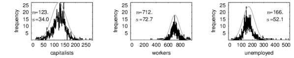
Figure 1: Class distributions: histograms of the number of actors in each economic class with a constant bin size of 1. The smooth lines are fitted normal distributions. On average approximately 71.2% of the population are workers, 12.3% are capitalists employing one worker or more, and the remaining 16.6% are unemployed.

The social stratification generated by capitalist economies is a complex phenomenon with systematic causal relations to the dominant social relations of production. In reality the social relations of production are more complex than the relations in the SR model (actors may receive combinations of wage and property income and therefore belong to more than one economic class, some actors are self-employed, others receive the majority of their income from rent, many people work for governments rather than private enterprises, and so forth). In consequence, some work is required to map empirical data on social stratification to the more basic categories employed here. It is equally clear, however, that the class of capitalists is numerically small, whereas the class of workers, that is those actors who predominately rely on wage income for their subsistence, constitute the vast majority of the population. The SR model should reflect this empirical fact. The class breakdown in the SR model can be measured according to the following rule:

Class size measure: After each year (an application of rule ${\bf 1Y}$) count the number of workers, $|W|$, capitalists, $|C|$, and unemployed, $|U|$.

Figure 1 is a histogram of class sizes generated by the model collected over the duration of the simulation. The number of workers, capitalists and unemployed are normally distributed. The normal distributions summarise a dynamic process that supports social mobility, where actors move between classes during their imputed lifetimes, occurring within a stable partition of the population into two main classes – a small employing class and a larger employed class. Fluctuations in class sizes are evidently mean-reverting, reflecting stable and persistent class sizes, given the exogenous and constant wage interval. The unemployment rate is higher than is usually reported in modern economies, but real measures of unemployment typically discount frictional unemployment, whereas here all non-employed actors are considered unemployed, and, in addition, there is no concept of self-employment. In conclusion, the SR model self-organises into a realistic partition of the working population into a minority of employers and a majority of employees.

3.2 Firm size distribution

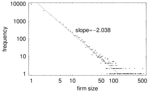
Figure 2: Firm size distribution: histogram of firm sizes by employees in log-log scale with a constant bin size of 1. The straight line is an ordinary least squares regression of the data and represents a power-law distribution $P(x)\propto x^{-(\alpha+1)}$ with exponent $\alpha=1.038$ for data collected over 15 simulated years. Axtell [5] reports $\alpha=1.059$ from data of approximately 5.5 million U.S. firms in 1997. The special case $\alpha=1$ is known as the Zipf distribution.

Axtell [5] analysed US Census Bureau data for US firms trading between 1988 and 1997 and found that the firm size distribution followed a special case of a power-law known as Zipf’s law, and this relationship persisted from year to year despite the continual birth and demise of firms and other major economic changes. During this period the number of reported firms increased from 4.9 million to 5.5 million. Gaffeo et. al. [19] found that the size distribution of firms in the G7 group over the period 1987-2000 also followed a power-law, but only in limited cases was the power-law actually Zipf. Fuijiwara et. al. [18] found that the Zipf law characterised the size distribution of about 260,000 large firms from 45 European countries during the years 1992–2001. A Zipf law implies that a majority of small firms coexist with a decreasing number of disproportionately large firms.

Firm sizes in the SR model are measured according to the following rule:

Firm sizes measure: After each month (an application of rule 1M) count the number of employees in each firm.

The SR model replicates the empirical firm size distribution. Figure 2 is a histogram of firm sizes. The straight line is a fit to the power-law:

$$P(x)\propto x^{-(\alpha+1)}$$ (3)

For data collected over a short time period, such as 15 simulated years, $\alpha$ approaches $1.0$. The special case $\alpha=1.0$ is Zipf, and hence the firm size distribution generated by the model is consistent with the empirical data. Data collected over shorter periods follows a power-law with exponent that deviates from 1.

The largest US firm in 1997 had approximately $10^{6}$ employees from a total reported workforce of about $10^{7}$ individuals [5]. Therefore, the largest firm size should not exceed about $\frac{1}{10}$th of the total workforce. Figure 2 shows that, with low but non-zero probability, a single firm can employ over half the workforce, representing a monopolisation of a significant proportion of the economy by a single firm, a clearly unrealistic occurrence. A possible reason for the over-monopolisation of the economy is the assumption that firms have a single capitalist owner, which conflates capital concentration with firm ownership. In reality, large firms normally have multiple owners and individual capitalists own multiple firms. Further, there are many technical reasons why particular firms do not grow beyond a certain size that are ignored in this model. A final point is that the probability of monopoly within the period of observation decreases with the number of actors; hence, if the simulation were run with $N=10^{7}$ actors (which is not possible due to insufficient computational resources) then it is unlikely that a single firm would employ half the workforce. Gaffeo et. al. [19] note that firms are distributed more equally during recessions than during expansions, which accounts for the yearly deviations from Zipf. This relationship has not been tested in the SR model.

3.3 Firm growth distributions

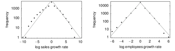
Figure 3: Firm size growth rate distribution: histogram of the log growth rates of firms per simulated year in linear-log scale with a constant bin size of 1. The LHS graph shows growth rates of firm sales. The RHS graph shows growth rates of employees. The solid lines are OLS regressions of the data and represent a Laplace (double-exponential) distribution $P(x)\propto e^{-|(x-\alpha)/\beta|}$. Refs. [24, 7, 43, 1, 3, 2, 15] report that log growth rates of sales and employees of US and Italian firms follow a Laplace distribution.

Stanley et. al. [43] and Amaral et. al. [1] analyzed the log growth rates of publicly traded US manufacturing firms in the period 1974 – 93 and found that growth rates, when aggregated across all sectors, appear to robustly follow a Laplace (double exponential) form. This holds true whether growth rates are measured by sales or number of employees. More precisely, if the annual growth rate is $r=\ln(\frac{s_{t+1}}{s_{t}})$, where $s_{t}$ is the size of a firm in year $t$, then for all years the probability density of $r$ is consistent with an exponential decay:

$$f(r)\propto\e^{-|\frac{r-\alpha}{\beta}|}$$ (4)

with some deviation from the Laplace distribution at high and low growth rates resulting in slightly ‘fatter wings’ [24, 3, 2]. Bottazzi and Secchi [7] replicate these findings and report a Laplace growth distribution for Italian manufacturing firms during the period 1989–96.

Firm growth in the SR model is measured according to:

Firm growth rate measure: After each year (an application of rule 1Y) calculate the current size, $s_{t}$, for a firm that traded at some point during the year. Size is measured in terms of number of employees or total sales revenue. The growth rate is $s_{t}/s_{t-1}$. (If a firm ceased trading during the year then $s_{t}=1$, and if a firm began trading during the year then $s_{t-1}=1$).

The SR model generates log annual growth rates for firms that are consistent with a Laplace distribution, whether growth is measured in terms of sales or number of employees. Figure 3 plots log growth rates in log-linear scale and reveals the characteristic ‘tent’ shape signature of a symmetric exponential decay. There is some deviation from a Laplace distribution for firms with shrinking sales, which may be due to noise or represent some non-accidental property. Bottazii and Secchi note that standard economic models do not predict a Laplace growth distribution and propose a stochastic model to explain the data that, in the abstract, shares similarities to firm growth in this model. Briefly, both models assume firm growth is a multiplicative stochastic process constrained by global resources (this kind of process is embedded in the general dynamics of the SR model). The SR model is intended to model the social relations of production, and therefore the replication of the empirical Laplace growth distribution suggests that the social relations of production play an important role in constraining the dynamics of firm growth.

Refs. [24, 15, 2, 3, 43] note that the standard deviation (std) of growth rates decreases as a power law with size, that is, $\ln\sigma(r)\sim-\beta\ln r$, where $\beta\approx 0.15$. The SR model does not replicate this finding given the specified wage interval. In fact, $\ln\sigma(r)$ appears to increase as a power law with size, although the data is quite noisy. However, the exponent of the power law is sensitive to the wage parameter, and it is possible to replicate the empirical relationship at lower average wages. Explanations of the relationship between growth variation and size assume that firms have internal structures such that increased size lessens market risk [2, 3], which contrasts with the simple firm structure employed in this model. Axtell in ref. [4] presents an agent-based model of the life-cycle of firms that replicates the Zipf size distribution, Laplace growth rates and power-law scaling of the std of growth. Firms in Axtell’s model have more complex internal relations between employees who make optimising decisions on the trade-off between effort and reward.

3.4 Firm demise distribution

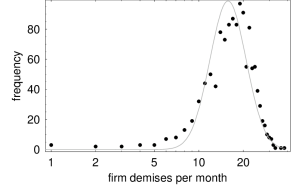
Figure 4: Firm demises distribution: Histogram of firm demises per simulated month in log-linear scale with a constant bin size of 1. The solid line is a fit to the lognormal distribution. Cook and Ormerod [10] report that the distribution of US firm demises per year during the period 1989 to 1997 is closely approximated by a lognormal distribution.

Cook and Ormerod [10] report that the distribution of US firm demises per year during the period 1989 to 1997 is closely approximated by a lognormal distribution, and note that the number of demises varies little from year to year with no clear connection to recession or growth.

The number of firm demises per month in the simulation is measured according to:

Firm demise measure: After each month (an application of rule 1M) count the number of firm demises that occurred during the month. A firm demise occurs when a firm fires all its employees.

Demises per month are measured rather than per year in order to avoid bucketing the data. Figure 4 is a histogram of firm demises per month with a fitted lognormal distribution. It shows that the model generates a distribution of firm demises that is approximated by a lognormal distribution and is therefore consistent with empirical findings.

According to Cook and Ormerod the average number of firms in the US during the period 1989 to 1997 was 5.73 million, of which on average 611,000 died each year. So roughly 10% of firms die each year. In the simulation on average 18 firms die each month and therefore on average 216 firms die each year, a figure in excess of the 123 firms that exist on average. So although the distribution of firm demises is consistent with empirical data, the rate at which firms are born and die is much higher than in reality. This is not too surprising when it is considered that the model entirely abstracts from the material nature of the goods and services processed by the economy and any persistent demand for them. In this model firms compete by playing a game of chance that models the unpredictability of a competitive economy. But the complete absence of the material side of the economy results in an unrealistic level of volatility in market interactions. The SR model must therefore be extended to include causal relations between the social architecture and the forces of production. Clearly there is a limit to what may be deduced from consideration of the social relations of production alone.

3.5 GDP growth

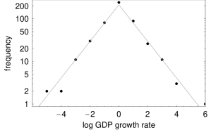
Figure 5: Rescaled GDP growth rate distribution: histogram of the log growth rate of GDP in linear-log scale with a constant bin size of 1. The solid lines are OLS regressions of the data and represent a Laplace (double-exponential) distribution $P(x)\propto e^{-|(x-\alpha)/\beta|}$. Ref. [24] reports that log GDP growth rates of 152 countries during the period 1950–92 follow a Laplace distribution.

Gross Domestic Product (GDP) measures the value of gross production at current prices, including consumption and gross investment. Lee at. al. [24] and Canning et. al. [9] analyse the GDP of 152 countries during the period 1950–52 and find that the distribution of GDP log growth rates is consistent with a Laplace distribution, and therefore conclude that firm growth and GDP growth are subject to the same laws [24].

The GDP growth rate in the SR model is measured according to the following rule:

GDP growth measure: At the close of year $t$ calculate the total firm income, $X_{t}$, received during that year (i.e., all income received during application of rule ${\bf M_{1}}$). The GDP growth rate is then $X_{t}/X_{t-1}$.

Empirical measurements of GDP must be detrended to remove the effects of inflation but this is unnecessary when measuring GDP in the model due to the assumption of a fixed amount of money.

Figure 5 plots log GDP growth rate for the simulated economy in log-linear scale. The data is noisy but consistent with a Laplace distribution when sampled over a period of 100 years so for clarity figure 5 contains data from an extended run of 500 years. The characteristic tent shape indicates that the SR model is consistent with the Laplace distribution of GDP growth.

Gatti et. al. in ref. [20] present an agent-based model of the life-cycle of firms that replicates the Zipf size distribution and Laplace growth rates of firms and aggregate output (GDP). They show that the power-law of firm size implies that growth is Laplace distributed and also that small micro-shocks can aggregate into macro-shocks to generate recessions. Firms in their model are not disaggregated into employees and employers and market shocks are exogenous, whereas in this model firms are composed of individuals and are subject to endogenous shocks that are the consequence of the competition for a finite amount of available market value, itself a product of income flows.

3.6 Duration of recessions

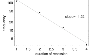
Figure 6: Recession duration distribution: Histogram of the frequency of the duration of recessions in log-linear scale with a constant bin size of 1. The solid line is a fit to an exponential distribution, $f(d)\propto\lambda e^{-\lambda d}$, with exponent $\lambda=1.22$, representing an average recession duration of 1.22 simulated years.

Wright [45], reinterpreting empirical data presented by Ormerod and Mounfield [33], concludes that the frequency of the duration of economic recessions, where a recession is defined as a period of shrinking GDP, follows an exponential law for 17 Western economies over the period 1871–1994. Recessions tend not to last longer than 6 years, the majority of recessions last 1 year, and for the US the longest recession has been only 4 years [34].

The duration of recessions in the simulation is measured according to the following rule:

Recession duration measure: A recession begins when

$X_{t}/X_{t-1}<1$

and ends when

$X_{t+k}/X_{t+k-1}\geq 1$

The duration of the recession is $k$ years.

The SR model is in close agreement with these empirical findings. Figure 6 is a histogram of the frequency of the duration of recessions collected over a period of 500 simulated years. The functional form of the frequency of duration of recessions is exponential, $f(d)\propto\lambda\e^{-\lambda d}$, with $\lambda=1.22$, which compares to a value of $\lambda=0.94$ for the empirical data [45]. The value of $\lambda$ is the average duration of a recession. Also, the duration of recessions in the model ranges from 1 to 4 simulated years.

3.7 Income shares

GDP is the sum of revenues received by firms during a single year. Firms pay the total wage bill, $W$, from this revenue. Hence the total value of domestic output is divided into a share that workers receive as wages, $X_{w}=\frac{W}{X}$, and the remainder that capitalists receive as profit, $X_{p}=1-X_{w}$. Advanced capitalist countries publish national income accounts that allow wage and profit shares to be calculated, which reveal some characteristic features. Shares in national income have remained fairly stable during the twentieth century, despite undergoing yearly fluctuations. For example, the profit share, normally lower than the wage share, is between 0.25 to 0.4 of GDP, although it occasionally can be as high as 0.5 (source: Foley and Michl’s calculations in ref. [17] for US, UK and Japan spanning a period of over 100 years; other authors place the wage share nearer to $\frac{1}{2}$, for example on average 0.54 between 1929 and 1941 for the USA [21] and similar in chapters 3 and 8 of ref. [16]).

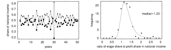
Figure 7: Wage and profit shares in national income. The LHS graph is a representative time series of the fluctuating shares in national income. GDP, denoted $X$, is the sum of revenues received by firms during a single year. The solid triangles are the wage share, $X_{w}$, which represents the sum total of wages paid to the working class, $W$, divided by GDP, $X_{w}=\frac{W}{X}$. The solid squares are the profit share, $X_{p}$, which represents the sum total of profits received by the capitalist class divided by GDP, $X_{p}=1-\frac{W}{X}$. The wage share fluctuates around a mean of 0.55 and the profit share fluctuates around a mean of 0.45. The RHS graph is a histogram of the ratio $\frac{W}{1-W}$. The smooth line is a fitted pdf of the ratio of two normal variates, which indicates that fluctuations of shares in national income are normally distributed around long-term stable means.

Income shares in the simulation are measured according to:

Income shares measure: Calculate the GDP, $X$, for the year. Count the total income received by workers during the same year (i.e., income received during application of rule ${\bf W_{1}}$), which is defined as the total wage bill $W$. The wage share is $X_{w}=\frac{W}{X}$, and the profit share is $X_{p}=1-X_{w}$.

Figure 7 is a plot of the shares in national income generated by the model. The profit share is generally lower than the wage share, and the yearly fluctuations are normally distributed about long-term stable values. Ignoring differences of definition, and for the purposes of a rough and ready comparison, the model generates an average profit share of 0.45, which compares well to the empirical data. The model therefore reproduces the empirical situation of fluctuations about a long-term stable mean, and additionally the profit and wage shares have realistic values, although it is an open question whether suitably de-trended fluctuations are normally distributed in capitalist economies.

3.8 Disaggregated income distributions

Income shares can be disaggregated and measured at the level of individuals in order to understand income differentiation within classes. The empirical income distribution is characterised by a highly unequal distribution of income, in which a very small number of households receive a disproportionate amount of the total (e.g., using wealth as an indicator of income, in 1996 the top 1% of individuals in the US owned 40% of the total wealth [26]). The higher, property-income, regime of the income distribution can be fitted to a Pareto (or power) distribution [25, 26, 28, 14, 30, 31, 41], whereas the lower, or wage-income, regime, which represents the vast majority of the population, is normally fitted to a lognormal distribution [41, 29, 6], but recently some researchers [31, 14, 13] report that an exponential (Boltzmann-Gibbs) distribution better describes the empirical data. Plotting the income distribution as a complementary cumulative distribution function (ccdf) in log-log scale reveals a characteristic ‘knee’ shape at the transition between the two regimes [28, 14, 13, 41, 31].

(a) The complete income distribution plotted as a ccdf in log-log scale. The data is binned at a constant size of 1. Note the characteristic ‘knee’ shape, a feature found in empirical distributions. The transition from the lognormal to the Pareto regime occurs between $P(x)=0.1$ and $P(x)=0.01$, which means that under 10% of incomes follow the Pareto law.

(b) The class components of the income distribution plotted as ccdfs in log-log scale. Note the long tail of the capitalist income distribution. Worker income is clustered around the average wage.

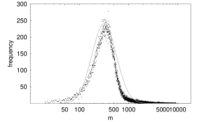
(c) The lower regime of the income distribution plotted in log-linear scale. The solid line is a fit to a lognormal distribution. The approximately lognormal distribution results from a mixture of wage income and small employer income.

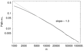
(d) The power law regime of the income distribution plotted as a ccdf in log-log scale. The straight line is a fit to the power (Pareto) law, $P(x)\propto x^{-(\alpha+1)}$, where $\alpha=1.3$.

Figure 8: Graphical analysis of the stationary income distribution. Incomes are measured over the duration of a year and the data is collected over the duration of the simulation.

The functional form of the income distribution is stable over many years, although the parameters seem to fluctuate within narrow bounds. For example, for property-income, the power-law, $P(x)\propto x^{-(\alpha+1)}$, has a value $\alpha=1.3$ for the UK in 1970 [25], $\alpha=[1.1,1.3]$ for Australia between 1993 and 1997 [28], $\alpha=1.7$ for US in 1998 [14], on average $\alpha=1.0$ for post-war Japan [30], and $\alpha=[0.5,1.5]$ for US and Japan between 1960 and 1999 [31]. In sum, the income distribution is asymptotically a power-law with shape parameter $\alpha\approx 1.0$, and this regime normally characterises the top 1% to 5% of incomes.

The two-parameter lognormal distribution

$$P(x)=\frac{1}{x\sigma\sqrt{2\pi}}\exp(\frac{-(\log\frac{x}{m})^{2}}{2\sigma^{2}})$$ (5)

where $m$ is the median, and $\beta=1/\sqrt{2\sigma^{2}}$ is the Gibrat index, can describe the remaining 95% or so of incomes. For example, for post-war Japan, the Gibrat index ranges between approximately $\beta=2.25$ and $\beta=3.0$ [41]. In contrast, if the lower income range is fitted to an exponential law

$$P(x)\propto\lambda\e^{\lambda x}$$ (6)

then by analogy with a perfect gas, from which the Boltzmann-Gibbs law originates, $\lambda$ is interpreted as an average economic ‘temperature’, which should be close to the average wealth in the economy, adjusting for the effects of the Pareto tail.

The SR model is in close qualitative and quantitative agreement with all these empirical facts. It also explains why there are two major income regimes, and provides a candidate explanation of why the distribution of low incomes is sometimes identified as either lognormal or exponential.

Incomes in the simulation are measured according to the following rule:

Incomes measure: After each year (an application of rule ${\bf 1Y}$) calculate the total income received by each actor during the year. Both wage income (from rule ${\bf W_{1}}$) and capitalist income (from rule ${\bf M_{1}}$) are counted as income.

Figure 8(a) is a plot of the stationary income ccdf generated by the model. It reproduces the characteristic ‘knee’ shape found in empirical income distributions. The ‘knee’ is formed by the transition from the lower regime, consisting mainly of the wealth of the working class and owners of small firms, to the higher regime, consisting mainly of the wealth of the capitalist class. The knee occurs at around $P(M\geq m)=0.1$, which means the power-law regime holds for at most 10% of incomes.

Figure 8(b) splits the income distribution according to class. The capitalist distribution has a long tail, qualitatively different from the worker distribution, which is clustered around the average wage. Figure 8(c) is a plot of the lower regime of the income distribution in log-linear scale fitted to a lognormal distribution with Gibrat index $\beta=1.42$. Figure 8(d) is a plot of the property-income regime in log-log scale. The straight line fit indicates that higher incomes asymptotically approach a power-law distribution of the form $P(x)\propto x^{-(\alpha+1)}$, with $\alpha=1.3$. The two income regimes are consequences of the two major sources of income in capitalist societies, that is wages and profits, and the overall income distribution is a mixture of two qualitatively different distributions. The lower regime is fitted better by a lognormal distribution rather than an exponential. The lognormal distribution, in this model, is not the result of stochastic multiplicative process, which is the explanation often proposed, but results from a mixture of normally distributed wage incomes and the profit-income of small firm owners. It is an open question whether the lognormal distribution found in empirical data can be similarly explained by the combined effect of income from employment and the income of small employers.

At first glance it appears that the model contradicts empirical evidence that the lower income regime is exponentially distributed. But if the stationary distribution of money holdings (i.e., instantaneous wealth) is measured, rather than income, a different picture emerges, which may help explain the lack of consensus in empirical studies. Wealth is measured according to the following rule:

Wealth measure: After each year (an application of rule ${\bf 1Y}$) calculate the total money held by each actor.

Figure 9 is a plot of the stationary money ccdf generated by the model. As before, figure 9(a) reproduces the characteristic ‘knee’ shape found in empirical income distributions. But in this case the lower regime is characterised by an exponential (or Boltzmann-Gibbs) distribution. The transition between regimes occurs approximately in the middle of the ccdf corresponding to a situation in which the total wealth in the economy is distributed approximately evenly between the classes. Figure 9(c) plots the workers’ money distribution in log-linear scale. The straight line fit reveals an exponential distribution of the form $P(x)=\lambda\e^{\lambda x}$, where $\lambda=0.017$, which is indeed close to the average wealth in the economy, $\lambda=\frac{M}{N}=0.01$ [12]. Figure 9(d) plots the capitalists’ money distribution in log-log scale. The straight line fit reveals a power-law distribution with similar exponent to that of income.

The higher income and wealth regimes are qualitatively identical, but the lower income and wealth regimes are qualitatively distinct. Measuring the lower end of income yields a lognormal distribution, whereas measuring the lower end of wealth yields an exponential. Income depends solely on monies received during an accounting period, whereas wealth depends on both income and spending patterns. The differences between the empirical studies could be due to differences in whether the measures employed are predominately income measures or wealth measures.

(a) The complete money distribution plotted as a ccdf in log-log scale. The transition from the Boltzmann-Gibbs to Pareto regime occurs in the middle of the ccdf. The data is binned at a constant size of 1.

(b) The class components of the money distribution plotted as ccdfs in log-log scale. Note the long tail of the capitalist money distribution.

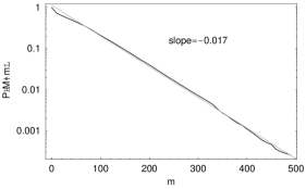
(c) A section of the workers’ money ccdf plotted in linear-log scale. The straight line is a fit to the exponential (Boltzmann-Gibbs) law, $P(x)=\lambda e^{\lambda x}$, where $\lambda=0.017$.

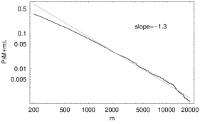
(d) A section of the capitalists’ money ccdf plotted in log-log scale. The straight line is a fit to the power (Pareto) law, $P(x)\propto x^{-(\alpha+1)}$, where $\alpha=1.3$.

Figure 9: Graphical analysis of the stationary money distribution. Money holdings are measured at the end of a year and the data is collected over the duration of the simulation.

The lognormal and power-law fits are only approximations to the true distributions, and a full analysis of the income distribution is postponed. However, a few brief points can be made. A popular explanation of the power-law tail of the income distribution is that it arises from an underlying stochastic multiplicative process, often thought to model the geometric growth of capital invested in financial markets [31, 30, 36, 37, 25, 26, 8]. The importance of financial markets in determining capital flows and hence capitalist income is undeniable. But the model developed here shows that an income power-law can arise from industrial capital invested in firms, absent financial markets that support capital reallocation between industries or between capitalists. Capitalist income, in this model, is not derived from investment in portfolios that provide a return, but is composed of the sum of values added via the employment of productive workers. In this sense, capitalist income is additive, not multiplicative. But workers are grouped in firms that follow a power-law of size. Hence, the power-law of capitalist income is due to a power-law in the network structure of the wage-capital relation. Di Matteo et. al. [28] show that an additive stochastic model of interacting agents on a power-law network generates power-law distributions, and presumably a similar explanation accounts for the capitalist income distribution generated by this model. Clearly, the firm ownership structure in this model is highly simplified, and it is an open question whether this conclusion holds in models that include joint ownership of firms.

3.9 Rate-of-profit distribution

Figure 10: Capital-weighted rate-of-profit distribution: Histogram of amount of capital invested that generated a given percentage profit rate within a simulated year. The data is collected over the duration of the simulation and binned at a constant size of 1. The average profit rate is 80.5% and the median profit rate is 64% (on average 1 coin invested returns 1.8 coins). Wells [44] measured the profit rate distribution of over 100,000 UK firms trading in 1981 and found that the distribution was right-skewed.

Farjoun and Machover [16] propose that the proportion of industrial capital (out of the total capital invested in the economy) that finds itself in any given rate-of-profit bracket will be approximated by a gamma distribution by analogy with the distribution of kinetic energy in a gas at equilibrium. The gamma distribution is a right-skewed distribution. Wells [44] measured the rate-of-profit distribution of over 100,000 UK firms trading in 1981 and found that in general the distribution was right-skewed, whatever precise definition of profit was used, although the data was not well characterised by a gamma distribution.

In reality capitalist owners of firms invest in both variable (wages) and constant capital (investment in commodity inputs to the production process and relatively long-lasting means of production) [32] and the rate-of-profit is calculated on the total capital invested. The SR model abstracts from the forces of production and hence capitalist owners invest only in variable capital (i.e. expenditures on wages due to the application of rule ${\bf W_{1}}$). Capitalists also spend income in the marketplace according to rule ${\bf E_{1}}$, and this expenditure could be interpreted as either consumption or investment in constant capital, but to theoretically ground the latter interpretation the model would need to be extended to include a determination of the distribution of ratios of constant to variable capital across firms. Rather than introduce the material side of the economy, which properly belongs to future substantive extensions of the model, the rate-of-profit in the simulation is calculated on variable capital alone. Hence rate-of-profit measures will exceed those found empirically.

The rate-of-profit distribution in the model is measured according to:

Profit rate measure: After each year (an application of rule ${\bf 1Y}$) calculate the profit rate for each firm trading at the close of the year. The profit rate, $p_{i}$, of firm $i$ is defined as

$$p_{i}=100\left(\frac{r_{i}}{w_{i}}-1\right)$$ (7)

where $r_{i}$ is the total revenue received during the year and $w_{i}$ is the total wages paid during the year.

Figure 11: Firm-weighted rate-of-profit distribution: Histogram of number of firms that generated a given percentage profit rate within a simulated year. The data is collected over the duration of the simulation and binned at a constant size of 1. Wells [44] measured the firm-weighted profit rate distribution of over 100,000 UK firms trading in 1981 and found that, similar to the capital-weighted rate-of-profit, the distribution was right-skewed, although less noisy.

Figure 10 graphs the amount of capital that returned a given profit within a year. Consistent with empirical research the distribution is highly right-skewed. Wells [44] reports that if the rate-of-profit is weighted according to number of firms, rather than capital invested, the distribution is also right-skewed and very similar in overall character, although less noisy. Figure 11 graphs the firm-weighted distribution from the simulation. It is also right-skewed, like the capital-weighted distribution, but considerably less noisy. The SR model provides the opportunity to deduce an analytical form for the industrial rate-of-profit distribution given additional assumptions on capital investment. As a step toward this goal an approximation to the firm-weighted rate-of-profit distribution in the SR model is now derived.

Consider a single firm that trades for a single year and has an average size of $s$ employees during this period. The firm samples the market on average $12s$ times during a year. This is a simplification, as during a year, firms are created and destroyed, and therefore do not necessarily interact with the marketplace over the whole year. The value of each market sample, $M_{i}$, is a function of the instantaneous money distribution, which is mixture of exponential and Pareto forms. Assume each $M_{i}$ is independent and identically distributed (iid) with mean $\mu_{m}$ and variance $\sigma_{m}^{2}$. During a month the same employee may be repeatedly selected, or not selected, due to the causal slack introduced by rule ${\bf 1M}$. Therefore the value generated per employee per month, $V_{i}$, is some function $f$ of $M_{i}$ independent of the firm size $s$. Simplifying further to avoid detailed consideration of the distribution of market samples per employee, assume that $f(x)=x+v$, where $v$ is a constant. Hence each $V_{i}$ is idd with mean $\mu_{1}=\mu_{m}+v$ and variance $\sigma_{1}^{2}=\sigma_{m}^{2}$. By the Central Limit Theorem the sum of the firm’s market samples in a year, which constitutes the total revenue, $R$, can be approximated by a normal distribution $R=\sum V_{i}\approx N(\mu_{r},\sigma_{r}^{2})$, where $\mu_{r}=12s\mu_{1}$ and $\sigma_{r}^{2}=12s\sigma_{1}^{2}$.

The firm’s total wage bill for the year, $W$, is the sum of $12(s-1)$ individual wage payments, $\omega_{i}$. Note that the capitalist owner does not receive wages. Each $\omega_{i}$ is iid according to a uniform distribution, $\omega_{i}\sim U(\omega_{a},\omega_{b})$, with mean $\mu_{2}=(\omega_{a}+\omega_{b})/2$ and variance $\sigma_{2}^{2}=(\omega_{b}-\omega_{a})^{2}/12$. By the Central Limit Theorem the wage bill, $W$, can be approximated by a normal distribution $W=\sum\omega_{i}\approx N(\mu_{w},\sigma_{w}^{2})$, where $\mu_{w}=12(s-1)\mu_{2}$ and $\sigma_{w}^{2}=12(s-1)\sigma_{2}^{2}$.

Define the ratio of revenue to the wage bill as $X=R/W$ and assume that $R$ and $W$ are independent. $X$ is the ratio of two normal variates and its pdf is derived by the transformation method to give:

$$f_{X}(x\mid s) = \frac{\exp\left[-\frac{1}{2}(\frac{\mu_{r}^{2}}{\sigma_{r}^{2}}+\frac{\mu_{w}^{2}}{\sigma_{w}^{2}})\right]}{4\pi k_{1}^{3/2}}$$ (8)

$$\left(2\sigma_{r}\sigma_{w}\sqrt{k_{1}}+\e^{\Lambda(x)}\sqrt{2\pi}(1+\Phi(\sqrt{\Lambda(x)}))(\mu_{w}\sigma_{r}^{2}+x\mu_{r}\sigma_{w}^{2})\right)$$

where

$$k_{1} = \sigma_{r}^{2}+x^{2}\sigma_{w}^{2}$$

$$\Lambda(x) = \frac{(\mu_{w}\sigma_{r}^{2}+x\mu_{r}\sigma_{w}^{2})^{2}}{2\sigma_{r}^{2}\sigma_{w}^{2}(\sigma_{r}^{2}+x^{2}\sigma_{w}^{2})}$$

$$\Phi(x) = \frac{2}{\sqrt{\pi}}\int_{0}^{x}\e^{-t^{2}}\d t$$

(8) is the pdf of the rate-of-profit conditional on the firm size $s$. The unconditional rate-of-profit distribution can be obtained by considering that firm sizes are distributed according to a Pareto (power-law) distribution:

$$f_{S}(s)=\frac{\alpha\beta^{\alpha}}{s^{\alpha+1}}$$

where $\alpha$ is the shape and $\beta$ the location parameter. Firm sizes in the model range between 1 (a degenerate case of an unemployed worker) to a maximum possible size $N$. Therefore the truncated Pareto distribution

$$g_{S}(s)=f_{S}(s\mid 1<S\leq N)=\frac{f(s)}{F(N)-F(1)}=\frac{s^{-(1+\alpha)}\alpha}{1-N^{-\alpha}}$$

where

$$f(s)=F^{\prime}(s)$$

is formed to ensure that all the probability mass is between 1 and $N$. By the Theorem of Total Probability the unconditional distribution $f_{X}(x)$ is given by:

$$f_{X}(x)=\int_{2}^{N}f_{X}(x\mid s)g_{S}(s)\d s$$ (9)

where the range of integration is between 2 and $N$ as firms of size 1 are a degenerate case that do not report profits. Expression (9) defines the $g_{S}(s)$ parameter-mix of $f_{X}(x\mid S=s)$. The rate-of-profit variate is therefore composed of a parameter-mix of a ratio of independent normal variates each conditional on a firm size $s$ that is distributed according to a power-law. Writing (9) in full yields:

$$f_{X}(x) = \int_{2}^{N}\frac{\exp\left[-6(\frac{s\mu_{1}^{2}}{\sigma_{1}^{2}}+\frac{(s-1)\mu_{2}^{2}}{\sigma_{2}^{2}})\right]}{2\pi\Theta^{3/2}(x)}$$ (10)

$$\left(k_{2}\sqrt{\Theta(x)}+\sqrt{6\pi}\Psi(x)\exp\left[\frac{6\Psi^{2}(x)}{k_{2}^{2}\Theta(x)}\right]\left(1+\Phi(\frac{\sqrt{6}\Psi(x)}{k_{2}\sqrt{\Theta(x)}})\right)\right)$$

$$\frac{s^{-(1+\alpha)}\alpha}{1-N^{-\alpha}}\;\d s$$

where

$$k_{2} = \sqrt{s\sigma_{1}^{2}}\sqrt{(s-1)\sigma_{2}^{2}}$$

$$\Theta(x) = s\sigma_{1}^{2}+(s-1)x^{2}\sigma_{2}^{2}$$

$$\Psi(x) = (s-1)s(\mu_{2}\sigma_{1}^{2}+x\mu_{1}\sigma_{2}^{2})$$

(10) is the pdf of $X=R/W$ but the rate-of-profit in the simulation is measured as $P=100\left(X-1\right)$. The pdf of P is therefore a linear transform of X:

$$f_{P}(x)=\frac{1}{100}f_{X}(1+\frac{x}{100})$$ (11)

(11) defines a distribution with 6 parameters: (i) the mean employee market sample $\mu_{1}$, (ii) the variance of the employee market sample $\sigma_{1}^{2}$, (iii) the mean wage $\mu_{2}$, (iv) the wage variance $\sigma_{2}$, (v) the Pareto exponent, $\alpha$, of the firm size distribution, and (vi) the number of economic actors $N$.

(11) is solved numerically to compare the distribution of the theoretically derived variate $P$ with the profit data generated by the SR model. The values of the parameters are measured from the simulation. In this particular case $\mu_{1}=\mu_{m}+v\approx 50+v$, $\sigma_{1}^{2}=\sigma_{m}^{2}\approx 55000$, $\mu_{2}\approx 50$, $\sigma_{2}^{2}\approx 533.3$, $\alpha\approx 1.04$ and $N=1000$. The best fit is achieved with $v=25$ coins. Figure 12 plots the pdf $f_{P}(x)$ with the rate-of-profit frequency histogram of Fig. 11 and shows a reasonable fit between the derived distribution and the data.

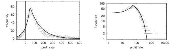
Figure 12: Theoretical fit to the firm-weighted rate-of-profit distribution. The solid lines plot the theoretical pdf $f_{P}(x)$ scaled by a constant in the frequency axis. The RHS graph plots the function and data in log-log scale and extends the range of the plot to the super-profit range. All profits in excess of 10000 are truncated, which accounts for the outlier at the maximum profit rate.

With some further work the 6-parameter distribution $f_{P}(x)$ could be fitted to empirical rate-of-profit measures and compared against other candidate functional forms. Although (11) ignores effects due to capital investment the interpretation of the parameters $\mu_{1}$, $\sigma_{1}^{2}$, $\mu_{2}$ and $\sigma_{2}^{2}$ can be extended to refer to the means and variances of revenue and cost per employee. A testable consequence of the SR model is the conjecture that the empirical rate-of-profit distribution will be consistent with a parameter-mix of a ratio of normal variates with means and variances that depend on a firm size parameter that is distributed according to a power law.

4 Discussion

The empirical coverage of the SR model is broad although the model can be formally stated in a small number of simple economic rules that control the dynamics. The model compresses and connects a large number of empirical facts within a single causal framework. But this paper only introduces the model and is merely a starting point for further analysis and investigation.

The enormous benefit of exploring computational models of phenomena is that the complex dynamic consequences of a set of causal rules can be automatically and correctly deduced by running a computer program that performs a computational deduction. In this case the deduction is from micro-economic social relations to emergent, macro-economic phenomena. But the reasons why a set of causal rules necessarily generate the observed dynamic consequences may initially be opaque precisely because a computer simulation is required to perform the deduction. This is why computational modelling is not an alternative to mathematical modelling but is intimately connected to it. To give just one example, within the parameter space explored, the SR model generates fluctuations in national income about long-term stable means. But it requires a mathematical deduction to understand why this necessarily occurs. The computational model unequivocally demonstrates that in principle such a deduction exists and its basic elements and assumptions will correspond to those of the computational model. Of course, a deductive proof may be more or less difficult to construct even if it is known to exist. So one use of computational modelling is to more easily identify candidate theories, which may then be further analysed to generate explanations in the form of mathematical deductions or natural language explanations, the aim being to understand why the dynamic consequences are logically necessary. An example of the potential of this approach is the deduction of a candidate functional form for the distribution of industrial profit. Contrast this situation to a purely mathematical approach, in which the investigator may only explore candidate theories that are directly amenable to mathematical deduction. This methodology is unnecessarily restrictive, particularly if the system presents difficult analytic challenges.

The model has something to say about a broad range of macro-economic phenomena that have already been intensively studied and theorised in standard economic theories, for example business cycle phenomena. The relationship between the model presented here and existing economic models of particular economic phenomena is a topic for further research. It is likely, for instance, that some of the stochastic models elaborated in the econophysics literature may be embedded within the overall dynamics of the SR model, particularly those that are more narrowly focussed on explaining certain distributions in isolation, such as firm size, income and company growth. However, a new requirement for more narrowly focussed models is they provide more detailed and exact explanations for particular phenomena than those provided by the broad but shallow SR model.

The fact that the empirical distributions considered can be deduced from the social relations of production alone suggests that some of the striking phenomena of a capitalist economy depend not so much on specifics but on very general and highly abstract structural features of that system. In consequence, existing theories may be looking in the wrong place for economic explanations, or at least introducing redundant considerations. Given this possibility, it is worth making a few comments to contrast the approach taken in this paper to standard approaches, if only to emphasise that this new approach is theoretically motivated.

The ontology of this model differs from standard economic models. Standard competitive equilibrium models, or neoclassical models, normally take as their starting point an ontology of rational actors that maximise self-interest in a market for scarce resources [11]. Attention is focussed on determining the equilibrium exchange ratios of commodity types, which are solutions to a set of simultaneous, static constraints. Historical time is absent, so equilibrium states are logically rather than causally derived, and typically money is not modelled. Neo-Ricardian models, in contrast, take as their starting point an ontology of technical production relations between commodity types that define the available material transformations that economic actors may perform. The production of commodities by means of commodities [42] results in a surplus product that is distributed to capitalists and workers [35]. Despite many essential differences, there are some important similarities between neo-classical and neo-Ricardian models. For example, prices in neo-Ricardian models are also exchange ratios determined by solutions to static, simultaneous constraints. Similarly, historical time is absent, so there is no causal explanation of how or why a particular configuration of the economy arose. Money only plays a nominal not a causal role. There are clear differences between, on the one hand, neo-classical and neo-Ricardian ontologies, and, on the other, the basic ontology of the model developed here. Most obvious is that commodity types and rational actors are absent. Instead, the model emphasises precisely those elements of economic reality that neo-classical and neo-Ricardian theories tend to ignore, specifically actor-to-actor relations mediated by money, which unfold in historical time, and result in dynamic, not static, equilibria. At a high level of abstraction, and at the risk of over simplification, neo-classical models theorise scarcity constraints, neo-Ricardian models theorise technical-production constraints, whereas this model theorises the dynamic consequences of social constraints, which are historically contingent facts about the way in which economic production is socially organised.

As argued elsewhere [16, 23] exclusive emphasis on the ontology of standard economic models is inimical to further progress in the field of political economy. The SR model constitutes constructive proof that the standard ontology is redundant for forming explanations of the empirical phenomena surveyed in this paper. This is not to assert that some other, perhaps more concrete issues, may require consideration of purposive activity for their explanation and hence the introduction of rational actors, or require consideration of technical production constraints and hence the introduction of commodity types. Rather, the claim is that, for the empirical aggregates considered, there is no need to perform the standard reduction of political economy to psychology and the technical conditions of production, and further, that the dominant causal factors at work are not to be found at the level of individual behaviour, nor are they to be found at the level of technical-production constraints, but are found at the level of the social relations of production, which constitute an abstract, but nevertheless real, social architecture that constrains the possible actions that purposive individuals may choose between, whether optimally or otherwise. This is why the actors in this model probabilistically choose between possible economic actions constrained only by their class status and current money endowments, an approach that is closer to the classical conception of political economy, in which individuals are considered to be representatives of economic classes that have definite relations to each other in the process of production. The social architecture, in particular the wage-capital social relation, dominates individuals, who, although free to make local economic decisions, do so in a social environment neither of their own choosing or control.

It may be objected that economic actors are clearly purposive and it is therefore essential to model individual rationality, even when considering macro-level phenomena. The underlying assumption of the rational actor approach to economics is that macro phenomena are reducible to and determined by the mechanisms of individual rationality. Farjoun and Machover [16] noted some time ago that the successful physical theory of statistical mechanics is in direct contradiction to this assumption. For example, classical statistical mechanics models the molecules of a gas as idealised, perfectly elastic billiard balls. This is of course a gross oversimplification of a molecule’s structure and how it interacts with other molecules. Yet statistical mechanics can deduce empirically valid macro-phenomena. Quoting Khinchin [22]:

Those general laws of mechanics which are used in statistical mechanics are necessary for any motions of material particles, no matter what are the forces causing such motions. It is a complete abstraction from the nature of these forces, that gives to statistical mechanics its specific features and contributes to its deductions all the necessary flexibility. … the specific character of the systems studied in statistical mechanics consists mainly in the enormous number of degrees of freedom which these systems possess. Methodologically this means that the standpoint of statistical mechanics is determined not by the mechanical nature, but by the particle structure of matter. It almost seems as if the purpose of statistical mechanics is to observe how far reaching are the deductions made on the basis of the atomic structure of matter, irrespective of the nature of these atoms and the laws of their interaction. (Eng. trans. Dover, 1949, pp. 8–9).

The method of abstracting from the mechanics of individual rationality, and instead emphasising the particle nature of individuals, is valid because the number of degrees of freedom of economic reality is very large. This allows individual rationality to be modelled as a highly simplified stochastic selection from possibilities determined by an overriding social architecture. The quasi-psychological motives that supposedly drive individual actors in the rational actor approach can be ignored because in a large ensemble of such individuals they hardly matter.

5 Conclusion

The aim was to understand the possible economic consequences of the social relations of production considered in isolation and develop a model that included money and historical time as essential elements. The theoretical motivation for the approach is grounded in Marx’s distinction between the invariant social relations of production and the varying forces of production. Standard economic models typically do not pursue this distinction. The model of the social relations of production replicates some important empirical features of modern capitalism, such as (i) the tendency toward capital concentration resulting in a highly unequal income distribution characterised by a lognormal distribution with a Pareto tail, (ii) the Zipf or power-law distribution of firm sizes, (iii) the Laplace distribution of firm size and GDP growth, (iv) the exponential distribution of recession durations, (v) the lognormal distribution of firm demises, and (vi) the gamma-like rate-of-profit distribution. Also, the model naturally generates groups of capitalists, workers and unemployed in realistic proportions, and business cycle phenomena, including fluctuating wage and profit shares in national income. The good qualitative and in many cases quantitative fit between model and empirical phenomena suggests that the theory presented here captures some essential features of capitalist economies, demonstrates the causal importance of the social relations of production, and provides a basis for more concrete and elaborated models. A testable conjecture is that measures of the empirical rate-of-profit distribution will be consistent with a parameter-mix of a ratio of normal variates with means and variances that depend on a firm size parameter that is distributed as a power-law.

A final and important implication is that the computational deduction outlined in this paper implies that some of the features of economic reality that cause political conflict, such as extreme income inequality and recessions, are necessary consequences of the social relations of production and hence enduring and essential properties of capitalism, rather than accidental, exogenous or transitory.

References

- [1] L. A. N. Amaral, S. V. Buldyrev, S. Havlin, H. Leschhorn, F. Maass, and M. A. Salinger. Scaling behavior in economics: I. empirical results for company growth. Journal de Physique I France, 7:621–633, 1997.
- [2] L. A. N. Amaral, P. Gopikrishnan, V. Plerou, and H. E. Stanley. A model for the growth dynamics of economic organizations. Physica A, 299:127–136, 2001.
- [3] Luis A. Nunes Amaral, Sergey V. Buldyrev, Shlomo Havlin, Philipp Maass, Michael A. Salinger, H. Eugene Stanley, and Michael H. R. Stanley. Scaling behavior in economics: the problem of quantifying company growth. Physica A, 244:1–24, 1997.
- [4] R. Axtell. The emergence of firms in a population of agents: local increasing returns, unstable nash equilibria, and power law size distributions. CSED working paper No.3, 1999.
- [5] Robert L. Axtell. Zipf distribution of u.s. firm sizes. Science, 293:1818–1820, 2001.
- [6] W. W. Badger. An entropy-utility model for the size distribution of income. In B. J. West, editor, Mathematical models as a tool for social science, pages 87–120. Gordon and Breach, New York, 1980.
- [7] Giulio Bottazzi and Angelo Secchi. Explaining the distribution of firms growth rates, 2003.
- [8] Jean-Philippe Bouchaud and Marc Mezard. Wealth condenstation in a simple model of economy. http://www.arXiv.org/abs/cond-mat/0002374.
- [9] D. Canning, L. A. N. Amaral, Y. Lee, M. Meyer, and H. E. Stanley. Scaling the volatility of gdp growth rates. Economics Letters, 60:335–341, 1998.
- [10] William Cook and Paul Ormerod. Power law distribution of the frequency of demises of us firms. Physica A, 324:207–212, 2003.
- [11] Gerard Debreu. Theory of value – an axiomatic analysis of economic equilibrium. Yale University Press, New Haven and London, 1959.
- [12] A. Dragulescu and V. M. Yakovenko. Statistical mechanics of money. The European Physical Journal B, 17:723–729, 2000.
- [13] A. Dragulescu and V. M. Yakovenko. Statistical mechanics of money, income and wealth: a short survey, 2002. http://arXiv.org/abs/cond-mat/0211175.
- [14] Adrian A. Dragulescu. Applications of Physics to economics and finance: money, income, wealth, and the stock market. PhD thesis, Department of Physics, University of Maryland, USA, 2003. http://arXiv.org/abs/cond-mat/0307341.
- [15] G. De Fabritiis, F. Pammolli, and M. Riccaboni. On size and growth of business firms. Submitted to Elsevier Science.
- [16] Emmanuel Farjoun and Moshe Machover. Laws of Chaos, a Probabilistic Approach to Political Economy. Verso, London, 1989.
- [17] Duncan K. Foley and Thomas R. Michl. Growth and Distribution. Harvard University Press, Cambridge, Massachusetts, 1999.
- [18] Yoshi Fujiwara, Corrado Di Guilmi, Hideaki Aoyama, Mauro Gallegati, and Waturu Souma. Do pareto-zipf and gibrat laws hold true? an analysis with european firms. http://www.arXiv.org/abs/cond-mat/0310061.
- [19] Edoardo Gaffeo, Mauro Gallegati, and Antonio Palestrini. On the size distribution of firms: additional evidence from the g7 countries. Physica A, 324:117–123, 2003.
- [20] Domenico Delli Gatti, Corrado Di Guilmi, Edoardo Gaffeo, Gianfranco Giulioni, Mauro Gallegati, and Antonio Palestrini. A new approach to business fluctuations: heterogenous interacting agents, scaling laws and financial fragility. To appear in Journal of Economic Behaviour and Organisation, 2003.
- [21] M. Kalecki. Theory of Economic Dynamics. Rinehart and Company Inc., New York, 1954.
- [22] Alexander I. Khinchin. Mathematical foundations of statistical mechanics. Dover Publications, 1949.
- [23] Tony Lawson. Economics and reality. Routledge, London and New York, 1997.
- [24] Youngki Lee, Luis A. Nunes Amaral, David Canning, Martin Meyer, and H. Eugene Stanley. Universal features in the growth dynamics of complex organizations. Physical Review Letters, 81(15):3275–3278, 1998.
- [25] M. Levy and S. Solomon. Of wealth power and law: the origin of scaling in economics. citeseer.nj.nec.com/63648.html.
- [26] Moshe Levy and Sorin Solomon. New evidence for the power-law distribution of wealth. Physica A, 242:90–94, 1997.
- [27] Karl Marx. Capital, volume 1. Progress Publishers, Moscow, 1954. Original English edition published in 1887.
- [28] T. Di Matteo, T. Aste, and S. T. Hyde. Exchanges in complex networks: income and wealth distributions. http://www.arXiv.org/abs/cond-mat/0310544.
- [29] E. W. Montroll and M. F. Shlesinger. Maximum entropy formalism, fractals, scaling phenomena, and 1/f noise: a tale of tails. Journal of Statistical Physics, 32:209–230, 1983.
- [30] Makoto Nirei and Waturu Souma. Income distribution and stochastic multiplicative process with reset events, 2003. http:// www.santanfe.edu/ makato/ papers/ income.pdf.
- [31] Makoto Nirei and Waturu Souma. Income distribution dynamics: a classical perspective, 2003. http://www.santafe.edu/ makato/papers/income.pdf.
- [32] N. Okishio. Constant and variable capital. In John Eatwell, Murray Milgate, and Peter Newman, editors, The New Palgrave – Marxian Economics, pages 91–103. W. W. Norton and Company, New York and London, 1990.
- [33] P. Ormerod and C. Mounfield. Power law distribution of the duration and magnitude of recessions in capitalist economies: breakdown of scaling. Physica A, 293:573–582, 2001.
- [34] Paul Ormerod. The us business cycle: power law scaling for interacting units with complex internal structure. Physica A, 314:774–785, 2002.
- [35] Luigi L. Pasinetti. Lectures on the theory of production. Columbia University Press, New York, 1977.
- [36] William J. Reed. The pareto law of incomes – an explanation and an extension, 2000.
- [37] William J. Reed. The pareto, zipf and other power laws. Economics Letters, 74:15–19, 2001.
- [38] I. I. Rubin. Essays on Marx’s Theory of Value. Black Rose Books, 1973. Russian edition published in 1928.
- [39] A. M. Shaikh. The transformation from marx to sraffa. In Ernest Mandel and Alan Freeman, editors, Ricardo, Marx, Sraffa – the Langston Memorial Volume, pages 43–84. Verso, London, 1984.
- [40] A. M. Shaikh. The empirical strength of the labour theory of value. In R. Bellofiore, editor, Marxian Economics: A Reappraisal, volume 2, pages 225–251. Macmillan, 1998.
- [41] Watura Souma. Physics of personal income. In Hideki Takayasu, editor, Empirical science of financial fluctuations: the advent of econophysics, Tokyo, 2000. Nihon Keizai Shimbun, Inc. http://arxiv.org/abs/cond-mat/0202388.
- [42] Piero Sraffa. Production of commodities by means of commodities. Cambridge University Press, Cambridge, 1960.
- [43] M. H. R. Stanley, N. L. A. Amaral, S. V. Buldyrev, S. Havlin, H. Leschhorn, P. Maass, M. A. Salinger, and H. E. Stanley. Scaling behavior in the growth of companies. Nature, 379:804–806, 1996.
- [44] Julian Wells. What is the distribution of the rate of profit? In IWGVT mini-conference at the Eastern Economic Association, New York NY, 2001.
- [45] Ian Wright. The duration of recessions follows an exponential not a power law. Submitted for publication, preprint at http:// xxx.lanl.gov/ PS_cache/ cond-mat/ pdf/ 0311/ 0311585.pdf, 2003.
- [46] Ian Wright. Simulating the law of value. Submitted for publication, preprint at http:// www.unifr.ch/ econophysics/ articoli/ fichier/ WrightLawOfValue.pdf, 2003.