Ising Model on Edge-Dual of Random Networks

Abstract

We consider Ising model on edge-dual of uncorrelated random networks with arbitrary degree distribution. These networks have a finite clustering in the thermodynamic limit. High and low temperature expansions of Ising model on the edge-dual of random networks are derived. A detailed comparison of the critical behavior of Ising model on scale free random networks and their edge-dual is presented.

I Introduction

It is evident that a variety of natural and artificial systems can be described in terms of complex networks, in which the nodes represent typical units and the edges represent interactions between pairs of units ab ; d ; n1 . Clearly, identifying structural and universal features of these networks is the first step in understanding the behavior of these systems ws ; ba ; asbs ; ajb ; n2 ; fdj . Intensive research in recent years has revealed peculiar properties of complex networks which were unexpected in the conventional graph theory b . Among these one can refer to the scale free behavior of degree distribution ba , $P(k)$, where degree denotes the number of nearest neighbors of a node. From another point of view one is interested in the effect of structural properties of complex network on the collective behavior of systems living on these networks bw ; g ; sv ; ak ; ja ; mb ; khk ; h . Percolation and Ising model (or in general Potts model) are typical examples of statistical mechanics which have intensively been studied on uncorrelated random networks with given degree distributions dgm ; nsw ; cnsw ; gdm ; lvvz ; cah ; cabh ; bp ; vm ; vw ; dgm1 . By uncorrelated random network we mean those in which the degree of two neighbors are independent random variables . These networks are identified only by a degree distribution, $P(k)$, and have the maximum possible entropy. The locally tree-like nature of these networks provides a good condition to apply the recurrence relations to study the collective behavior of interesting modelsbax ; dgm ; dgm1 . It is seen that, depending on the level at which the higher moments of $P(k)$ become infinite, one encounters different critical behaviors that could be derived from a landau-Ginzburg theorygdm . This in turn reflects the mean field nature of these behaviors.

In this paper we are going to study the Ising model on the edge-dual of uncorrelated random networks with a given degree distribution. These kinds of networks have already been introduced in the context of graph theoryb . Given a network $G$, its edge-dual $\tilde{G}$ can be constructed as follows, see also figure(1): one puts a node in place of each edge of $G$ and connects each pair of these new nodes if they are emanating from the same node of $G$.
Such networks have been useful among other things for the study of maximum matching problem zy as well as topological phase transitions in random networkspdfv .
The interesting point about these networks is that they have generally a large degree of clustering even when the underlying network is tree-like. Due to this high clustering direct study of structural properties of such networks or of physical models defined on them is usually very difficult. However one can use this duality to adopt the techniques used in the context of random networks (e.g. the generating function formalism nsw ; cnsw ) and obtain interesting results for such networks rkm . For example it was shown in rkm that the edge-dual of a random scale free network with $P(k)\propto k^{-\gamma}$ will be a network whose degree distribution behaves like $\tilde{P}(k)\propto k^{-\tilde{\gamma}}$ for large degrees where $\tilde{\gamma}=\gamma-1$.

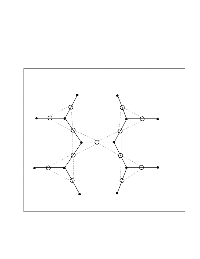
Figure 1: Some part of the edge-dual of a Bethe lattice with $z=3$. Empty circles and dotted lines denote the nodes and the edges of the edge-dual network respectively.

Our basic result is depicted in table 1, where we have compared the critical behavior of Ising model on scale free networks and their edge-dual networks. On the way to this basic result we have also studied as a preliminary step the Ising model on the edge-dual of Bethe lattices. We have also developed a systematic high and low temperature expansion for the Ising model on edge-dual networks for arbitrary degree distributions.
Moreover as a byproduct we have also shown that there is a simple relation between the partition function of an Ising model on a tree in which each spin interacts with its nearest and next nearest neighbors and the partition function of an Ising model on its edge-dual with only nearest neighbor interactions but in the presence of magnetic field.

The paper is organized as follows. In section II a relationship between the Ising model on a tree and on its edge-dual is derived. High and low temperature expansions of the partition function of the Ising model on the edge-dual of a random network are given in section III. In section IV we use recurrence method for the study of Ising model on the edge-dual of Bethe lattices. The same method is applied in section V to study the critical behavior of Ising model on the edge-dual of scale free networks. The conclusions are presented in section VI.

II A Relation Between Ising Model on a Tree And Its Edge-Dual Network

Let us consider an Ising model (with values of spin taking only $\pm 1$) on a tree graph $G$ with nearest and next nearest neighbor interactions of strength $J_{1}$ and $J_{2}$ in the absence of magnetic field. The hamiltonian is

$$E=-J_{1}\sum_{<ij>_{1}}S_{i}S_{j}-J_{2}\sum_{<ij>_{2}}S_{i}S_{j},$$ (1)

where $<ij>_{1}$ and $<ij>_{2}$ denote the nearest and next nearest neighbors respectively. For any given configuration of spins we can assign a unique configuration of spin variables (again taking values $\pm 1$) to the edges of the graph: any edge which connects two nodes having the variables $S_{i}$ and $S_{j}$ is assigned a value $S_{(ij)}:=S_{i}S_{j}$, see figure (2). On the other hand for any configuration of spins on the edges, ${S_{(ij)}}$, there are two possible configuration of spins on the nodes, which are obtained by flipping all the spins $S_{i}$ on the graph. Therefore there is a two to one correspondence between the spin configurations on the nodes of the graph and the edges of the graph.

Now if we write the above hamiltonian in terms of spins of edges we get

$$E=-J_{1}\sum_{<ij>_{1}}S_{(ij)}-J_{2}\sum_{<ij>_{2}}S_{(ik)}S_{(kj)},$$ (2)

where $k$ is the common nearest neighbor of nodes $i$ and $j$. But this is the hamiltonian of an Ising model on $\tilde{G}$, the edge-dual of the tree, with nearest neighbor interactions of strength $\tilde{J_{1}}=J_{2}$ in presence of a magnetic field of magnitude $\tilde{h}=J_{1}$.

$$\tilde{E}=-\tilde{h}\sum_{\tilde{i}}S_{\tilde{i}}-\tilde{J_{1}}\sum_{<\tilde{i}\tilde{j}>_{1}}S_{\tilde{i}}S_{\tilde{j}},$$ (3)

where $\tilde{i}$ and $\tilde{j}$ now denote the nodes of the edge-dual graph. Taking into account the relation between configurations mentioned above we obtain

$$Z(J_{1},J_{2},h=0,T)=2\tilde{Z}(\tilde{J_{1}}=J_{2},\tilde{J_{2}}=0,\tilde{h}=J_{1},T),$$ (4)

in which $Z$ and $\tilde{Z}$ are respectively the partition functions of the Ising model on $G$ and $\tilde{G}$ and $T$ denotes the temperature. We should stress that the above relation is true only for tree graphs, since the presence of loops in $G$ puts constraints on the values of spins which are assigned to the nodes of $\tilde{G}$. That is for any loop in $G$, the product of spins on its edges (equivalently the nodes of $\tilde{G}$) should be $+1$. Taking into account all these constraints makes the calculation of the partition function very difficult in the general case.

In the thermodynamic limit the two models have the same free energy density, that is $f=\tilde{f}$, where $f:=\frac{-T\ln Z}{N}$ and $\tilde{f}:=\frac{-T\ln\tilde{Z}}{\tilde{N}}$ are respectively the free energy of the Ising model on tree and its edge-dual. Here we have set the Boltsmann constant equal to one. Note that for a tree graph, $\tilde{N}=N-1$. Moreover, it is easy to see that the average magnetization of a spin in $\tilde{G}$

$$\tilde{m}=-\frac{\partial\tilde{f}}{\partial\tilde{h}}$$ (5)

is equal to the average correlation of two neighboring spins in $G$

$$<S_{i}S_{j}>=\frac{-\partial f}{\partial J_{1}}.$$ (6)

Knowing the average magnetization of spins in $\tilde{G}$ as a function of magnetic field, we can write the free energy density from equation (5) as follows bax

$$\tilde{f}(\tilde{J_{1}},\tilde{h},T)=\int_{\tilde{h}}^{\infty}(\tilde{m}(h^{\prime})-1)dh^{\prime}-\tilde{J_{1}}-\tilde{h}.$$ (7)

Differentiation of the right hand side with respect to $\tilde{h}$ correctly gives the magnetization $\tilde{m}$ and the integration constant $-\tilde{J_{1}}-\tilde{h}$ can be understood from the fact that for very large magnetic fields when the first integral vanishes, the partition function is dominated by the configurations where all the spins are up, and hence the free energy per site is given by $-\tilde{J_{1}}-\tilde{h}$.
Obviously if we replace $\tilde{J_{1}}$ with $J_{2}$ and $\tilde{h}$ with $J_{1}$ we obtain $f$, the free energy per site of Ising model on $G$ with nearest and next nearest neighbor interactions. In this way any nonanalytic behavior of $\tilde{f}$ will appear in $f$ too.

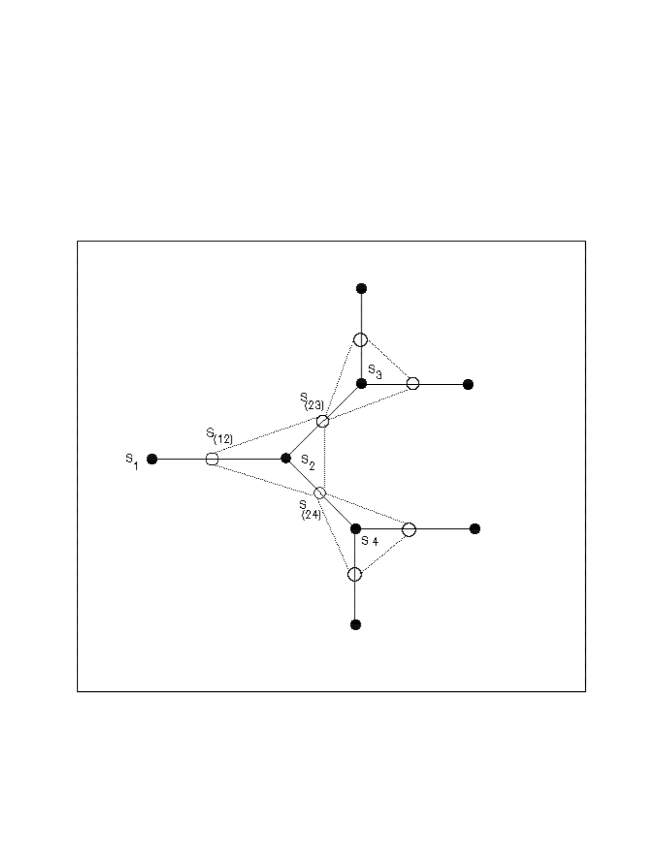
Figure 2: To each edge $(ij)$ we can assign a spin which is defined as the product of spins at the end point nodes of that edge i.e. $S_{(ij)}:=S_{i}S_{j}$.

III High And Low Temperature Expansions of Ising Model on Edge-Dual Networks

Consider a random network which we denote by $G$. We assume that the probability of each node having degree $k$ is equal to $P(k)$. Furthermore we assume that there is no correlations between the degrees of adjacent neighbors. The average number of nearest neighbors will be denoted by $n_{1}:=<k>=\sum_{k}kP(k)$. Degree distribution of nearest neighborscnsw is given by $\Pi(k)=\frac{kP(k)}{<k>}$. Thus the average number of next nearest neighbors will be $n_{2}:=<k>\sum_{k}(k-1)\Pi(k)=<k^{2}>-<k>$.
The edge-dual of such a network is denoted by $\tilde{G}$. Correspondingly every quantity pertaining to the dual network $\tilde{G}$ will be designated by a tilde sign.
In the following we will study the Ising model with only nearest neighbor interactions on $\tilde{G}$. The partition function is

$$\tilde{Z}=\sum_{\{S_{\tilde{i}}\}}e^{\tilde{K}\sum_{<\tilde{i}\tilde{j}>}S_{\tilde{i}}S_{\tilde{j}}},$$ (8)

where the sum in the exponential is over the nearest neighbors on the edge-dual of $G$. Here we have used the notation $\tilde{K}:=\frac{\tilde{J}}{T}$.

III.1 High Temperature Expansion

The above partition function can be written in a form appropriate for a high temperature expansionbax . To this end we write the exponential in the form

$$e^{\tilde{K}\sum_{<\tilde{i}\tilde{j}>}S_{\tilde{i}}S_{\tilde{j}}}=\cosh^{\tilde{L}}(\tilde{K})\prod_{<\tilde{i}\tilde{j}>}(1+S_{\tilde{i}}S_{\tilde{j}}\tanh(\tilde{K})),$$ (9)

where $\tilde{L}:=\frac{Nn_{2}}{2}$ is the number of edges in the $\tilde{G}$. Inserting this in equation (8) and expanding the product we get a series of terms each corresponding to a subgraph of $\tilde{G}$. Summing over spin configuration only terms which represent closed loops will survive bax and we arrive at the following expression for the partition function

$$\tilde{Z}=\cosh^{\tilde{L}}(\tilde{K})2^{\tilde{N}}\sum_{{\rm{closed\ loops\ c}}}\tilde{\eta}^{\tilde{L}(c)},$$ (10)

where $\tilde{\eta}=\tanh(\tilde{K})$, $\tilde{N}=\frac{Nn_{1}}{2}$ is the number of nodes of $\tilde{G}$ and $\tilde{L}(c)$ is the perimeter (the number of edges) of the closed loop $c$.

Clearly at high temperatures the first and the second terms corresponding to triangles and squares need be kept in the expansion.

$$\tilde{Z}=\cosh^{\tilde{L}}(\tilde{K})2^{\tilde{N}}(\tilde{N}_{\triangle}\tilde{\eta}^{3}+\tilde{N}_{\diamondsuit}\tilde{\eta}^{4}+\ldots.)$$ (11)

The number of triangles in $\tilde{G}$ has two parts: first, each triangle of $G$ appears as a triangle in $\tilde{G}$ too. Secondly, by definition of the edge-dual network, every triple of edges emanating from the same node in $G$ make a triangle in $\tilde{G}$. The number of the latter types of triangles is given by the number of distinct choices of three edges of a node, summed over the nodes of $G$. Thus

$$\tilde{N}_{\triangle}=N_{\triangle}+\sum_{i}(\begin{array}[]{c}k_{i}\\ 3\\ \end{array}),$$ (12)

in which $k_{i}$ is the degree of node $i$ in $G$. Since in an uncorrelated random network the number of triangles is a finite quantity in the thermodynamic limit cpv , we can neglect the first term compared with the second one which has an infinite contribution in this limit. The same argument is applicable to the case of squares so we can approximate these numbers by

$$\tilde{N}_{\triangle}\approx\sum_{i}(\begin{array}[]{c}k_{i}\\ 3\\ \end{array})=\frac{N}{3!}\sum_{k}k(k-1)(k-2)P(k),$$ (15)

$$\tilde{N}_{\diamondsuit}\approx\sum_{i}(\begin{array}[]{c}k_{i}\\ 4\\ \end{array})=\frac{N}{4!}\sum_{k}k(k-1)(k-2)(k-3)P(k).$$ (18)

Note that these relations become exact in the case of tree structures even for finite $N$.

III.2 Low Temperature Expansion

We now return to equation (8), the original relation for the partition function. Note that we can rewrite it as

$$\tilde{Z}=\sum_{\{S_{(ij)}\}}e^{\frac{\tilde{K}}{2}\sum_{i}((\sum_{j|i}S_{(ij)})^{2}-k_{i})},$$ (19)

where the first sum in the exponential is over nodes of $G$ and the second is over nearest neighbors of that node. Let us write $\tilde{Z}$ in a simpler way

$$\tilde{Z}=e^{-\tilde{K}L}\sum_{\{S_{(ij)}\}}e^{\frac{\tilde{K}}{2}\sum_{i}m_{i}^{2}},$$ (20)

where $L$ is the number of edges in $G$ and $m_{i}:=\sum_{j|i}S_{(ij)}$. Using the following identity

$$e^{\frac{\tilde{K}}{2}m_{i}^{2}}=\frac{1}{\sqrt{\frac{2\pi}{\tilde{K}}}}\int dx_{i}e^{-\frac{\tilde{K}}{2}({x_{i}}^{2}+2m_{i}x_{i})},$$ (21)

we find

$$\tilde{Z}=e^{-\tilde{K}L}(\frac{\tilde{K}}{2\pi})^{N/2}\sum_{\{S_{(ij)}\}}\int Dxe^{-\frac{\tilde{K}}{2}\sum_{i}(x_{i}^{2}+2x_{i}m_{i})},$$ (22)

where $Dx=\prod_{i}dx_{i}$ and $i$ runs over all the nodes of $G$. We can now perform the sum over the spin configurations in the integrand. To this end we note in view of the definition of $m_{i}$

$$\sum_{\{S_{(ij)}\}}e^{-\tilde{K}\sum_{i}x_{i}m_{i}}=\sum_{\{S_{(ij)}\}}e^{-\tilde{K}\sum_{<ij>}(x_{i}+x_{j})S_{(ij)}}$$ (23)

where $\sum_{<ij>}$ sums over all the links of $G$. The sum can be transformed to

$$\prod_{<ij>}(e^{-\tilde{K}(x_{i}+x_{j})}+e^{\tilde{K}(x_{i}+x_{j})})$$ (24)

$$= e^{\tilde{K}\sum_{<ij>}(x_{i}+x_{j})}\prod_{<ij>}(1+e^{-2\tilde{K}(x_{i}+x_{j})})$$ (25)

$$= e^{\tilde{K}\sum_{i}k_{i}x_{i}}\prod_{<ij>}(1+e^{-2\tilde{K}(x_{i}+x_{j})})$$ (26)

Putting all these together we find

$$\tilde{Z}=e^{-\tilde{K}L}(\frac{\tilde{K}}{2\pi})^{N/2}\int Dxe^{-\frac{\tilde{K}}{2}\sum_{i}(x_{i}^{2}-2k_{i}x_{i})}\prod_{<ij>}(1+e^{-2\tilde{K}(x_{i}+x_{j})}).$$ (27)

The product $\prod_{<ij>}(1+e^{-2\tilde{K}(x_{i}+x_{j})})$ can now be expanded as a series of terms each corresponding to a subgraph $g$ of $G$.

For any node $i$ of a the graph $G$, a factor $e^{-2Kz_{i}x_{i}}$ should be taken into account in which $z_{i}$ is the degree of that node in the subgraph. If a node $i$ dose not belong to the subgraph, $z_{i}=0$. Any subgraph determines uniquely the sequence of integers $\{z_{i};i=1,\ldots N\}$. Note that $z_{i}\leq k_{i}\ \ \ \forall i$. For each such sequence the integral can be easily calculated yielding

$$\tilde{Z}=e^{-\tilde{K}L+\frac{\tilde{K}}{2}\sum_{i}k_{i}^{2}}\sum_{{\rm g}}e^{-2\tilde{K}\sum_{i}z_{i}(k_{i}-z_{i})}.$$ (28)

It is the central result of this subsection which can be used for a low temperature expansion of Ising model on $\tilde{G}$. This formula incidentally shows that each subgraph $g$ and its complement (the graph obtained when one removes all the links of $g$ from $G$) give the same contribution to the partition function.

At very low temperatures, $\tilde{K}\longrightarrow\infty$, only the empty graph for which all $z_{i}=0$ and its complement for which all $z_{i}=k_{i}$ contribute yielding

$$\tilde{Z_{0}}=2e^{-\tilde{K}L+\frac{\tilde{K}}{2}\sum_{i}{k_{i}}^{2}}=2e^{-\tilde{K}L+\frac{\tilde{K}}{2}N\sum_{k}k^{2}P(k)}=2e^{-\tilde{K}\frac{N}{2}\langle k\rangle+\frac{\tilde{K}}{2}N\langle k^{2}\rangle}$$ (29)

resulting in a free energy per site equal to

$$\tilde{f_{0}}=-\frac{\tilde{J}}{2}(\langle k^{2}\rangle-\langle k\rangle)$$ (30)

where we have used the relation $\tilde{K}=\frac{\tilde{J}}{T}$.
The next to leading order term comes from subgraphs which have only one link, (we multiply their contribution by 2 to account for their complements). This will give

$$\tilde{Z}=\tilde{Z}_{0}(1+\sum_{<ij>}e^{-2\tilde{K}(k_{i}+k_{j}-2)}+\cdots)$$ (31)

where the sum is over all the links of $G$. This can be written as follows

$$\tilde{Z}=\tilde{Z}_{0}(1+N\frac{\langle k\rangle}{2}e^{4\tilde{K}}\ll e^{-2\tilde{K}(k+k^{\prime})}\gg+\cdots)$$ (32)

where $\ll\gg$ denotes the average with respect to the two point function $P(k,k^{\prime})$, the probability of two nodes of degrees $k$ and $k^{\prime}$ to be neighbors. For uncorrelated networks one has $P(k,k^{\prime})=(2-\delta_{k,k^{\prime}})\Pi(k)\Pi(k^{\prime})$. This procedure can be followed for higher order contributions.

IV Ising Model on Edge-Dual of Bethe Lattices

The Bethe Lattice bax is defined as a regular network where all nodes have the same degree $z$. Let us consider Ising spins on the edges of this network and let them interact with an external magnetic field $\tilde{h}$ and with each other if their corresponding edges are incident on the same node of the Bethe lattice. We can write the average magnetization of a spin lying on an arbitrary edge using the following recurrence relationbax

$$\tilde{m}=\frac{e^{\tilde{H}}g_{+}^{2}(0)-e^{-\tilde{H}}g_{-}^{2}(0)}{e^{\tilde{H}}g_{+}^{2}(0)+e^{-\tilde{H}}g_{-}^{2}(0)},$$ (33)

where $\tilde{H}:=\frac{\tilde{h}}{T}$ and $g_{+}(0)$ and $g_{-}(0)$ are respectively the partition functions for the system of spins on one side of the central spin when it is up or down. That is

$$g_{S}(0)=\sum_{\{S_{R}\}}e^{\tilde{K}\sum_{\tilde{i}|S}SS_{\tilde{i}}+\tilde{K}\sum_{<\tilde{i}\tilde{j}>}S_{\tilde{i}}S_{\tilde{j}}+\tilde{H}\sum_{\tilde{i}}S_{\tilde{i}}},$$ (34)

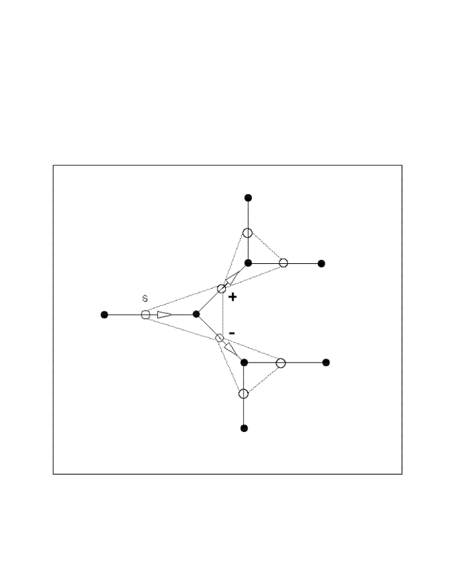
Figure 3: The partition function of spins on the branch stems from $S$ can recursively be written in terms of the partition functions of branches now stem from nearest neighbors of $S$.

where as before $\tilde{K}:=\frac{\tilde{J}}{T}$. Note that in this partition function only spins on one side of $S$ (for instance the right hand side spins, denoted by $\{S_{R}\}$) appear. Similar to $g_{S}(0)$ one can define a partition function $g_{S}(l)$ which gives the partition function of the branch of the lattice which stems from a node at layer $l$ where the value of its spin has been fixed to $S$. These partition functions can be related to each other recursively as follows, see also figure (3): in the right hand of $S$ there are $z-1$ spins which interact with $S$ and with each other. We can write $g_{S}(l)$ as a sum over different configurations of these spins. For each configuration we will have a term proportional to $g_{+}^{r}(l+1)g_{-}^{z-1-r}(l+1)$ where $r$ will be the number of up spins in such a configuration. Moreover we have to consider another factor which takes into account the Boltzmann factor associated to this configuration of spins. Energy of a configuration in which $r$ of these spins are up is the sum of three parts, a part given by their interaction with the external magnetic field equal to $-\tilde{h}(2r-z+1)$, a part from their interactions with spin $S$ equal to $-\tilde{J}(Sr-S(z-1-r))$ and finally a part given by interactions between themselves equal to $-\tilde{J}(\frac{r(r-1)}{2}+\frac{(z-1-r)(z-1-r-1)}{2}-r(z-1-r))$. Summing up the above arguments we arrive at

$$g_{S}(l)=\sum_{r=0}^{z-1}(\begin{array}[]{c}z-1\\ r\\ \end{array})e^{\tilde{H}(2r-z+1)+\tilde{K}(S(2r-z+1)-2r(z-1-r)+\frac{(z-1)(z-2)}{2})}g_{+}^{r}(l+1)g_{-}^{z-1-r}(l+1).$$ (35)

Returning to equation (33), magnetization of the central spin can be rewritten in a simpler form

$$\tilde{m}=\frac{e^{2\tilde{H}}-x_{0}^{2}}{e^{2\tilde{H}}+x_{0}^{2}}=\frac{e^{2\tilde{H}}-e^{-2y_{0}}}{e^{2\tilde{H}}+e^{-2y_{0}}},$$ (36)

where we have defined $x_{l}:=\frac{g_{-}(l)}{g_{+}(l)}=:e^{-y_{l}}$. When the magnetic field is positive we have $g_{-}(l)<g_{+}(l)$ thus $y_{l}$ is a positive quantity which plays a role similar to the magnetic field and thus can be interpreted as the local field experienced by a spin at distance $l$ from the central spin $S$. Now using equation (35), the recurrence relation for $y_{l}$ reads

$$y_{l}=-ln\left(\frac{\sum_{r}(\begin{array}[]{c}z-1\\ r\\ \end{array})e^{(\tilde{2H}+y_{l+1})r+\tilde{K}(z-1-2r-2r(z-1-r))}}{\sum_{r}(\begin{array}[]{c}z-1\\ r\\ \end{array})e^{(\tilde{2H}+y_{l+1})r+\tilde{K}(2r-z+1-2r(z-1-r))}}\right).$$ (37)

Setting $\tilde{H}=0$ and starting from distant ($l\gg 1$) spins with $y\ll 1$ one could obtain the values of $y$ for deeper spins in a step by step manner using the above relation until one arrives at $y_{0}$. Equation (36) tells us that we will have magnetization in this case only if $y_{0}$ is different from zero. It is evident that a stable nonzero solution for $y_{0}$ is possible only when the right hand side of the recurrence relation for $y_{l}$( when plotted versus $y_{l+1}$) has a slope greater than or equal to $1$. The equality will provide the critical temperature of the system which turns out to be given by

$$\frac{\sum_{r}r(\begin{array}[]{c}z-1\\ r\\ \end{array})e^{-\tilde{K}_{c}2r(z-1-r)}2\sinh(\tilde{K}_{c}(2r-z+1))}{\sum_{r}(\begin{array}[]{c}z-1\\ r\\ \end{array})e^{\tilde{K}_{c}(z-1-2r(z-r))}}=1.$$ (38)

Unfortunately it is not possible to derive a closed relation for $\tilde{K}_{c}$. In figure (4) we have computed this quantity numerically and compared it with the corresponding quantity in the Bethe lattice itself. In the latter case the critical temperature reads bax

$$\tanh{K_{c}}=\frac{1}{z-1}.$$ (39)

As figure (4) shows $\tilde{T}_{c}$ is much grater than $T_{c}$ which is as expected due to the larger number of interactions in the edge-dual network. In the figure we also show a linear fit, $\tilde{T}_{c}=a_{0}+a_{1}z$, to the numerical data for $\tilde{T}_{c}$ with $a_{0}=-3.53\pm 0.02$ and $a_{1}=1.97\pm 0.002$. As long as the critical behavior of the system is concerned we expect to see a standard mean field behavior as in the usual Ising model in spatial dimensions greater than $d_{c}=4$. We will further discuss these issues in the next section.

Figure 4: $T_{c}$( in units of $J$) for the Ising model on Bethe lattices(lower curve) and their edge-dual(upper curve).

V Ising Model on Edge-Dual of Random Networks

In this section we generalize the results of the previous section to the case of Ising model on the edge-dual of random networks with a given degree distribution $P(k)$. In this case a spin on the edge of such a random network will encounter $k_{1}-1$ and $k_{2}-1$ nearest neighbors at its right and left hand sides respectively. These numbers are random variables given by the degree distribution of nearest neighbors in the random network $\Pi(k)$.

V.1 General Arguments

Along the lines of section IV we can write the magnetization of a spin on an edge of random network with end point nodes of degrees $k_{1}$ and $k_{2}$ as

$$\tilde{m}_{k_{1}k_{2}}=\frac{e^{2\tilde{H}}-e^{-y_{0}(k_{1})-y_{0}(k_{2})}}{e^{2\tilde{H}}+e^{-y_{0}(k_{1})-y_{0}(k_{2})}},$$ (40)

where now $y$’s are random variables depending on distance and degree of end point nodes. Obviously magnetization of an arbitrary spin is given by

$$\tilde{m}=\sum_{k_{1},k_{2}}\Pi(k_{1})\Pi(k_{2})\frac{e^{2\tilde{H}}-e^{-y_{0}(k_{1})-y_{0}(k_{2})}}{e^{2\tilde{H}}+e^{-y_{0}(k_{1})-y_{0}(k_{2})}}.$$ (41)

As before here we used the notation $x_{l}(k):=e^{-y_{l}(k)}$ and $x_{l}(k):=\frac{g_{-}(l;k)}{g_{+}(l;k)}$ where $g_{S}(l;k)$ is the partition function for the cluster beyond the spin $S$ at distance $l$ from the central spin. As in the case of Bethe lattices (figure (3)) these quantities can be related to $g_{S^{\prime}}(l+1;k^{\prime})$’s by the following relations

$$g_{S}(l;k)=\sum_{r=0}^{k-1}e^{\tilde{H}(2r-k+1)+\tilde{K}(S(2r-k+1)-2r(k-1-r)+\frac{(k-1)(k-2)}{2})}\sum_{r/k-1}\prod_{a=1}^{r}g_{+}(l+1;k_{a})\prod_{b=r+1}^{k-1}g_{-}(l+1;k_{b}),$$ (42)

where the second sum is over different selections of $r$ distinct spins from the set of $k-1$ neighboring spins after assigning indices $1$ to $r$ to them. Thus the relation for $x_{l}(k)$ gets the form

$$x_{l}(k)=\frac{\sum_{r=0}^{k-1}e^{\tilde{H}2r+\tilde{K}(k-1-2r-2r(k-1-r))}\sum_{k-1-r/k-1}\prod_{a=1}^{k-1-r}x_{l+1}(k_{a})}{\sum_{r=0}^{k-1}e^{\tilde{H}2r+\tilde{K}(2r-k+1-2r(k-1-r))}\sum_{k-1-r/k-1}\prod_{a=1}^{k-1-r}x_{l+1}(k_{a})},$$ (43)

or in terms of $y$’s

$$y_{l}(k)=-ln(\frac{\sum_{r=0}^{k-1}e^{\tilde{H}2r+\tilde{K}(k-1-2r-2r(k-1-r))}\sum_{k-1-r/k-1}e^{-\sum_{a=1}^{k-1-r}y_{l+1}(k_{a})}}{\sum_{r=0}^{k-1}e^{\tilde{H}2r+\tilde{K}(2r-k+1-2r(k-1-r))}\sum_{k-1-r/k-1}e^{-\sum_{a=1}^{k-1-r}y_{l+1}(k_{a})}}).$$ (44)

Let us also derive a relation for the average energy of Ising model on the edge-dual of random networks in the absence of magnetic field. First note that we can write this quantity as a sum over the interaction energy associated to the spins on the edges emanating from the same node of $G$, that is

$$\tilde{E}=\sum_{i}e_{i}=\sum_{i}(\sum_{<(ij)(ik)>}-\tilde{J}S_{(ij)}S_{(ik)}).$$ (45)

Thus the thermodynamic average of the above quantity reads

$$<\tilde{E}>=N\sum_{k}P(k)<e_{k}>,$$ (46)

where $<e_{k}>$ is the average energy associated to a node of degree $k$. We are able to write this quantity in terms of $g$’s by summing over different configurations of spins on the edges of such a node. As before we sum over configurations in which $r$ spins out of these $k$ spins are up. For each such configuration we include an appropriate Boltzmann weight as before.
Denoting by $e_{k}:=-\tilde{J}(\frac{r(r-1)}{2}+\frac{(k-r)(k-r-1)}{2}-r(k-r))$ the interaction energy of these spins we obtain

$$<e_{k}>=\frac{\sum_{r=0}^{k}e_{k}e^{\tilde{K}(\frac{r(r-1)}{2}+\frac{(k-r)(k-r-1)}{2}-r(k-r))}\sum_{r/k}\prod_{a=1}^{r}g_{+}(0;k_{a})\prod_{b=r+1}^{k}g_{-}(0;k_{b})}{\sum_{r=0}^{k}e^{\tilde{K}(\frac{r(r-1)}{2}+\frac{(k-r)(k-r-1)}{2}-r(k-r))}\sum_{r/k}\prod_{a=1}^{r}g_{+}(0;k_{a})\prod_{b=r+1}^{k}g_{-}(0;k_{b})}.$$ (47)

After some algebra this relation takes the following simpler form in terms of $y$’s

$$<e_{k}>=-\tilde{J}\left(\frac{k(k-1)}{2}-\frac{\sum_{r=0}^{k}2r(k-r)e^{-\tilde{K}2r(k-r)}\sum_{k-r/k}e^{-\sum_{a=1}^{k-r}y_{0}(k_{a})}}{\sum_{r=0}^{k}e^{-\tilde{K}2r(k-r)}\sum_{k-r/k}e^{-\sum_{a=1}^{k-r}y_{0}(k_{a})}}\right).$$ (48)

Equations (41), (44) and (48) are the exact relations for magnetization, effective fields $y$ and energy of the system.

V.2 The Effective Medium Approximation

In this section we simplify the relations obtained in the previous subsection using the effective medium approximation dgm ; dgm1 applied satisfactorily to the study of Ising model on uncorrelated random networks. It is believed that this approximation takes in a good way into account the effects of high degree nodes which play an essential role in determining the critical behavior of the system specifically in inhomogeneous network having scale free degree distribution.
To this end we rewrite the relations derived above as if $y$’s are independent of $k$, the degree of the end pint nodes. This is achieved if we use the same $g$ for all the spins which are at the same distance from the central spin. The only explicit dependence on $k$ enters equation (44) which must be averaged over using the degree distribution of nearest neighbors $\Pi(k)$. We emphasize that this approximation is exact if we expand our relations for small $y$’s and keeping only the linear term. Note that we are finally interested in the critical behavior of the system where $y$’s tend to zero and thus we expect the above approximation to work well in the critical region. Consequently we use the following relations to extract the critical behavior of Ising Model on the edge-dual of an uncorrelated random network;

$$\tilde{m}_{=}\frac{e^{2\tilde{H}}-e^{-2y_{0}}}{e^{2\tilde{H}}+e^{-2y_{0}}},$$ (49)

for the magnetization,

$$y_{l}=-\sum_{k}\Pi(k)ln\left(\frac{\sum_{r=0}^{k-1}(\begin{array}[]{c}k-1\\ r\\ \end{array})e^{(2\tilde{H}+y_{l+1})r+\tilde{K}(k-1-2r-2r(k-1-r))}}{\sum_{r=0}^{k-1}(\begin{array}[]{c}k-1\\ r\\ \end{array})e^{(2\tilde{H}+y_{l+1})r+\tilde{K}(2r-k+1-2r(k-1-r))}}\right),$$ (50)

for the recurrence relations defining $y$’s and

$$<\tilde{E}>=-N\tilde{J}\sum_{k}P(k)\left(\frac{k(k-1)}{2}-\frac{\sum_{r=0}^{k}(\begin{array}[]{c}k\\ r\\ \end{array})2r(k-r)e^{-\tilde{K}2r(k-r)+y_{0}r}}{\sum_{r=0}^{k}e^{-\tilde{K}2r(k-r)+y_{0}r}}\right).$$ (51)

for the average of energy in the absence of magnetic field.

At this stage it is instructive to note that we can obtain the correlation between the central spin and a spin at distance $l$ by takin derivative of $\tilde{m}$ with respect to $\tilde{H}_{l}$, the magnetic field acting on such a spin. To this end we need also to label the magnetic fields along with the $y$’s in the above relations. Indeed in equations (49) and (50) the magnetic field has a similar index to that of y. On the other hand we have

$$\tilde{\chi}_{l}:=\frac{\partial\tilde{m}}{\partial\tilde{H}_{l}}|_{\{\tilde{H}_{l}=0\}}=\tilde{n}_{l}\tilde{G}_{c}(0,l),$$ (52)

where $\tilde{n}_{l}=2(\frac{<k^{2}>-<k>}{<k>})^{l}$ is the number of spins at distance $l$ from the central spin in the edge-dual of random network and $\tilde{G}_{c}(0,l):=<SS_{l}>-<S><S_{l}>$. Note that susceptibility is given by $\tilde{\chi}=\sum_{l}\tilde{\chi}_{l}$ where from (52) and (49) $\tilde{\chi}_{l}$ reads

$$\tilde{\chi}_{l}=\frac{\partial\tilde{m}}{\partial y_{0}}\prod_{i=0}^{l-2}(\frac{\partial y_{i}}{\partial y_{i+1}})\frac{\partial y_{l-1}}{\partial\tilde{H}_{l}}|_{\{\tilde{H}_{l}=0\}}.$$ (53)

If spins are deep enough in the network we can take all the $y$’s equal to each other, so for their derivatives. After making this approximation we obtain

$$\tilde{\chi}_{l}=\frac{\partial\tilde{m}}{\partial y_{0}}(\frac{\partial y_{i}}{\partial y_{i+1}})^{-1}\frac{\partial y_{l-1}}{\partial\tilde{H}_{l}}e^{-\frac{l}{\tilde{\lambda}}}|_{\{\tilde{H}_{l}=0\}},$$ (54)

where

$$\tilde{\lambda}:=-\frac{1}{ln(\frac{\partial y_{i}}{\partial y_{i+1}})}.$$ (55)

Here the index $i$ is only to distinguish between $y$’s in two subsequent shells and we will eventually set all the $y$’s equal to each other. This quantity is determined from the fixed point of equation (50). Consequently the length scale $\tilde{\lambda}$ is determined from equation (55) and as expected, it will become infinite in the critical point, that is when $\frac{\partial y_{i}}{\partial y_{i+1}}=1$. It is this critical behavior that gives rise to the critical behavior of $\tilde{\chi}$. Note however that $\tilde{\lambda}$ is not the correlation length which is determined from the long distance behavior of $\tilde{G}_{c}(0,l)$.

V.3 The critical behavior

Using equation (50) it is not difficult to see that $y_{0}$ is nonzero only for temperatures less than $\tilde{T}_{c}$ which satisfies

$$\sum_{k}\Pi(k)\frac{\sum_{r=0}^{k-1}r(\begin{array}[]{c}k-1\\ r\\ \end{array})e^{-\tilde{K}_{c}2r(k-1-r)}2\sinh(\tilde{K}_{c}(2r-k+1))}{\sum_{r}(\begin{array}[]{c}k-1\\ r\\ \end{array})e^{\tilde{K}_{c}(k-1-2r(k-r))}}=1.$$ (56)

It is a simple generalization of equation (38). This equation tells us that if $\tilde{K}_{c}\rightarrow 0$, i.e. at high temperatures, we have $\tilde{K}_{c}\sim\frac{<k>}{<k^{2}>-<k>}$. In other words the critical temperature of the system becomes infinite only when the second moment of $P(k)$ is infinite. This is the same behavior observed in uncorrelated random networks dgm ; lvvz . Thus even the finite value of clustering of edge-dual networks can not significantly alter the critical point although $\tilde{T}_{c}\gg T_{c}$ as we saw in the case of Bethe lattices in section IV.

Now let us limit ourselves to the critical region where $y$, $\tilde{H}$ and $\tilde{\tau}:=|\frac{T-\tilde{T}_{c}}{\tilde{T}_{c}}|$ are very small. We want an expansion of $\tilde{m}$, $y$ and $<\tilde{E}>$ in terms of small deviations from the critical point. First note that if we change the sign of $\tilde{H}$ , then by definition the sign of $y$ changes too and thus the magnetization is reversed. On the other hand, energy does not change under this change of sign. Any expansion of these quantities in terms of $\tilde{H}$ and $y$ must satisfy these symmetries. We summarize these arguments in the following expansions

$$\tilde{m}\approx\tilde{H}+y$$ (57)

$$y\approx a_{1}(2\tilde{H}+y)+a_{3}(2\tilde{H}+y)^{3}$$

$$<\tilde{E}>\approx b_{0}+b_{2}y^{2},$$

where the coefficients $a_{1},a_{3},b_{0}$ and $b_{2}$, are found to be

$$a_{1}=1+O(<k^{4}>)\tilde{\tau}\hskip 28.45274pta_{3}\sim O(<k^{4}>)$$ (58)

$$b_{0}\sim O(<k^{2}>)\hskip 28.45274ptb_{2}\sim O(<k^{4}>).$$

In this equation the averages are taken with respect to the degree distribution of random network $P(k)$. To be more specific let us consider a definite degree distribution, that is the well known scale free distribution $P(k)\propto k^{-\gamma}$. We consider several cases depending on the value of $\gamma$.

V.3.1 The case $\gamma>5$

In this case the edge-dual network behaves as a scale free network rkm , with $\tilde{\gamma}=\gamma-1>4$. Moreover, all the coefficients appearing in the expansions of (57) are finite. It is easy to show using equations (57) and (58) that $y$ is given by following relations

$$y\sim\tilde{\tau}^{\frac{1}{2}}\hskip 28.45274pt\tilde{H}=0$$ (59)

$$y\sim\tilde{H}^{\frac{1}{3}}\hskip 28.45274pt\tilde{\tau}=0$$

$$y\sim\frac{\tilde{H}}{\tilde{\tau}}\hskip 28.45274pt\tilde{H}\neq 0,\tilde{\tau}\neq 0.$$

The critical behavior of the other quantities can easily be derived from these relations

$$\tilde{m}\sim\tilde{\tau}^{\frac{1}{2}},\hskip 14.22636pt\delta\tilde{C}\sim cons.,\hskip 14.22636pt\tilde{\chi}\sim\tilde{\tau}^{-1}\hskip 28.45274pt\tilde{H}=0$$ (60)

$$\tilde{m}\sim\tilde{H}^{\frac{1}{3}}\hskip 28.45274pt\tilde{\tau}=0,$$

where $\delta\tilde{C}$ is the change of specific heat through the critical point. Here we have only shown dependence of interesting quantities on $\tilde{\tau}$ and $\tilde{H}$. Clearly these behaviors are those of the standard mean field model seen in the Ising model in spatial dimensions greater than $d_{c}=4$. This behavior is also seen in the case of Ising model on uncorrelated scale free random networks with $\gamma>5$ dgm ; lvvz .
Note that due to the finiteness of all the moments of degree distribution in Bethe lattices, the critical behavior of Ising model on their edge-dual network also lies in this class.

V.3.2 The case $\gamma=5$

Now $\tilde{\gamma}=4$. Some of the coefficients in expansions of (57) become infinite. To avoid these divergences which are an artifact of our expansion, we set a cut off for degrees which is proportional to $\frac{1}{y}$. Indeed in our expansion we used the fact that $ky\ll 1$ where $k$ is the degree of a nearest neighbor. Fortunately we are interested in the critical behavior where $y\rightarrow 0$ and the the above arguments work well in that region dgm .
Considering the above arguments, we find

$$y\sim\tilde{\tau}^{\frac{1}{2}}\hskip 28.45274pt\tilde{H}=0$$ (61)

$$y\sim(\frac{\tilde{H}}{ln(\tilde{H})})^{\frac{1}{3}}\hskip 28.45274pt\tilde{\tau}=0$$

$$y\sim\frac{\tilde{H}}{\tilde{\tau}ln(\tilde{\tau})}\hskip 28.45274pt\tilde{H}\neq 0,\tilde{\tau}\neq 0.$$

Thus the interesting quantities behave as

$$\tilde{m}\sim\tilde{\tau}^{\frac{1}{2}},\hskip 14.22636pt\delta\tilde{C}\sim ln(\tilde{\tau}),\hskip 14.22636pt\tilde{\chi}\sim\frac{1}{\tilde{\tau}ln(\tilde{\tau})}\hskip 28.45274pt\tilde{H}=0$$ (62)

$$\tilde{m}\sim(\frac{\tilde{H}}{ln(\tilde{H})})^{\frac{1}{3}}\hskip 28.45274pt\tilde{\tau}=0.$$

V.3.3 The case $3<\gamma<5$

In this case the degree distribution of edge-dual network will have the exponent $2<\tilde{\gamma}<4$. Again we have to take into account the divergences appearing in the expansion coefficients. From equations (57) and (58) we find

$$y\sim\tilde{\tau}^{\frac{1}{2}}\hskip 28.45274pt\tilde{H}=0$$ (63)

$$y\sim\tilde{H}^{\frac{8-\gamma}{9}}\hskip 28.45274pt\tilde{\tau}=0$$

$$y\sim\frac{\tilde{H}}{\tilde{\tau}^{\frac{\gamma-3}{2}}}\hskip 28.45274pt\tilde{H}\neq 0,\tilde{\tau}\neq 0.$$

And for the thermodynamic quantities we find

$$\tilde{m}\sim\tilde{\tau}^{\frac{1}{2}},\hskip 14.22636pt\delta\tilde{C}\sim\tilde{\tau}^{\frac{\gamma-5}{2}},\hskip 14.22636pt\tilde{\chi}\sim\tilde{\tau}^{-\frac{\gamma-3}{2}}\hskip 28.45274pt\tilde{H}=0$$ (64)

$$\tilde{m}\sim\tilde{H}^{\frac{8-\gamma}{9}}\hskip 28.45274pt\tilde{\tau}=0.$$

We do not consider the case $\gamma\leq 3$ since in this region $\tilde{\gamma}\leq 2$ and the average number of neighbors is infinite in the edge-dual network although it is still finite in the corresponding random network.

The above results show that these critical behaviors are very different from the ones seen in the uncorrelated scale free networks dgm ; lvvz , see table 1 . For example here the magnetization always behaves like the standard mean field case , $\tilde{m}\sim\tilde{\tau}^{\frac{1}{2}}$, but in uncorrelated scale free networks this behavior is only seen for $\gamma>5$ where all quantities are of the standard mean field type dgm ; lvvz .

	Magnetization	Specific heat	Susceptibility
$\gamma>5$	$\tilde{\tau}^{\frac{1}{2}}\left(\tau^{\frac{1}{2}}\right)$ $\ \ \tilde{H}^{\frac{1}{3}}$	cons.$\left(cons.\right)$	$\tilde{\tau}^{-1}\left(\tau^{-1}\right)$
$\gamma=5$	$\tilde{\tau}^{\frac{1}{2}}\left((\frac{\tau}{ln(\tau)})^{\frac{1}{2}}\right)$ $\ \ (\frac{\tilde{H}}{ln(\tilde{H})})^{\frac{1}{3}}$	$ln(\tilde{\tau})\left(\frac{1}{ln(\tau)}\right)$	$\frac{1}{\tilde{\tau}ln(\tilde{\tau})}\left(\tau^{-1}\right)$
$3<\gamma<5$	$\tilde{\tau}^{\frac{1}{2}}\left(\tau^{\frac{1}{\gamma-3}}\right)$ $\ \ \tilde{H}^{\frac{8-\gamma}{9}}$	$\tilde{\tau}^{\frac{\gamma-5}{2}}\left(\tau^{\frac{5-\gamma}{\gamma-3}}\right)$	$\tilde{\tau}^{\frac{3-\gamma}{2}}\left(\tau^{-1}\right)$

Table 1: Comparison of the critical behavior of Ising model on scale free random networks dgm (written inside parenthesis) and its edge-dual network.

VI Conclusion

In summary we studied the Ising model with nearest neighbor interactions on the edge-dual of uncorrelated random networks. We stated a simple relation between the partition function of this model and that of an Ising model with next nearest neighbor interactions on a tree-like network. High and low temperature expansions of the partition function were also derived. As a simple example we studied the Ising model on the edge-dual of Bethe lattices using the well known recurrence relation procedure. We finally generalized this study to the edge-dual of uncorrelated random networks. Although the critical temperature of Ising model on edge-dual network is higher than the one in the random network, both quantities become infinite in the same point, that is when the second moment of the degree distribution of random network, $<k^{2}>$, becomes infinite. This fact reflects the robustness of edge-dual networks against thermal fluctuations, a property which can be attributed to the large number of triangles and the special structure of the edge-dual networks. We also derived the critical behavior of Ising model on edge-dual network of an uncorrelated random scale free network. The results show that this behavior is significantly different from the one seen in the uncorrelated random networks.

Acknowledgment

The author is grateful to V. Karimipour for helpful discussions and useful suggestions.

References

- (1) R. Albert and A.-L.Barabási, Rev. Mod. Phys. 74,47-97 (2002).
- (2) S.N.Dorogovtsev and J.F.F.Mendes, Evolution of Networks : From Biological Nets to the Internet and WWW, (Oxford University Press, 2003).
- (3) M.E.J.Newman, SIAM Review 45, 167-256 (2003).
- (4) D.J.Watts and S.H.Strogatz , Nature 393,440 (1998).
- (5) A.-L.Barabási and R. Albert, Science 286, 509 (1999).
- (6) L.A.N.Amaral, A. Scala, M.Barthélémy, and H.E.Stanly, Proc. Natl. Acad. Sci USA 97,11149(2000).
- (7) R.Albert, H.Jeong, and A.-L.Barabási, Nature 406, 378(2000)
- (8) M.E.J.Newman, Phys. Rev. Lett. 89, 208701 (2002).
- (9) I. Farkas, I. Derenyi, H. Jeong, Z. Neda, Z. N. Oltvai, E. Ravasz, A. Schubert, A.-L. Barabasi, T. Vicsek, Physica A, 314 (2002) 25-34.
- (10) B.Bollobas, 1979, Graph theory, an introductory course, Springer-Verlag.
- (11) A.Barrat, M.Weigt, Eur. Phys. J. B 13, 547(2000).
- (12) M.Gitterman, J.Phys.A:Math Gen. 33, 8373(2000).
- (13) R. Pastor-Satorras, A. Vespignani, Phys. Rev. Lett. 86, 3200 (2001)
- (14) G. Abramson, M. Kuperman , Phys. Rev. E 63, 0309001(R) (2001).
- (15) S. Jalan, R. E. Amritkar, Phys. Rev Lett. 90, 014101 (2003)
- (16) M. Argollo de Menezes, A-L. Barabasi, cond-mat/0306304
- (17) B. Kozma, M. B. Hastings, G. Korniss , cond-mat/0309196.
- (18) M. B. Hastings,cond-mat/0304530.
- (19) A.V.Goltsev,S.N.Dorogovtsev and J.F.F.Mendes, Phys. Rev. E 67, 026123 (2003).
- (20) M.E.J.Newman, S.H.Strogatz and D.J.Watts, Phys. Rev. E 64, 026118 (2001).
- (21) D.S.Callaway,M.E.J.Newman, S.H.Strogatz and D.J.Watts, Phys. Rev. Lett. 85, 5468-5471 (2000).
- (22) S.N.Dorogovtsev, A.V.Goltsev and J.F.F.Mendes, Phys.Rev. E 66, 016104 (2002).
- (23) M.Leone, A.Vázquez, A.Vespignani and R.Zecchina, cond-mat/0203416.
- (24) R.Cohen, D. ben-Avraham and S.Havlin, Phys. Rev. E 66, 036113 (2002).
- (25) N. Schwartz, R. Cohen, D. ben-Avraham, A.-L. Barabasi, S. Havlin, Phys. Rev. E 66, 015104 (2002).
- (26) M.Boguñá and R.Pastor-Satorras, Phys. Rev. E 66, 047104 (2002).
- (27) A.Vázquez, Y.Moreno, Phys. Rev. E 67, 015101(R) (2003).
- (28) A.Vázquez and M.Weigt, Phys. Rev. E 67, 027101 (2003).
- (29) S.N. Dorogovtsev, A.V. Goltsev, J.F.F. Mendes, cond-mat/0310693.
- (30) R.J.Baxter, Exactly Solved Models in Statistical Mechanics(Academic Press, London, 1982).
- (31) H. Zhou, Z.-c. Ou-Yang , cond-mat/0309348.
- (32) G. Palla, I. Derenyi, I. Farkas, T. Vicsek, cond-mat/0309556.
- (33) A. Ramezanpour, V. Karimipour, A. Mashaghi, Phys. Rev. E 67, 046107 (2003).
- (34) G. Caldarelli, R. Pastor-Satorras, A. Vespignani, cond-mat/0212026.