Abstract

The quantum $XY$ model shows a Berezinskii-Kosterlitz-Thouless (BKT) transition between a phase with quasi long-range order and a disordered one, like the corresponding classical model. The effect of the quantum fluctuations is to weaken the transition and eventually to destroy it. However, in this respect the mechanism of disappearance of the transition is not yet clear. In this work we address the problem of the quenching of the BKT in the quantum $XY$ model in the region of small temperature and high quantum coupling. In particular, we study the phase diagram of a 2D Josephson junction array, that is one of the best experimental realizations of a quantum $XY$ model. A genuine BKT transition is found up to a threshold value $g^{\star}$ of the quantum coupling, beyond which no phase coherence is established. Slightly below $g^{\star}$ the phase stiffness shows a reentrant behavior at lowest temperatures, driven by strong nonlinear quantum fluctuations. Such a reentrance is removed if the dissipation effect of shunt resistors is included.

Berezinskii-Kosterlitz-Thouless
transition in Josephson junction arrays BKT transition in JJA

and

1 Introduction

Two-dimensional (2D) arrays of Josephson junction (JJA) are one of the best experimental realizations of a model belonging to the $XY$ universality class and permit to check and study a variety of phenomena related to both the thermodynamics and the dynamics of vortices. In these systems a Berezinskii-Kosterlitz-Thouless (BKT) transition [1] separates low-temperature superconducting (SC) state from the normal (N) state, the latter displaying no phase coherence [2]. At nanoscale size of the junctions, the quantum fluctuations of the superconducting phases cause new interesting features. These appear to be the consequence of the non-negligible energy cost of charge transfer between SC islands. Indeed small capacitances are involved and the phase and charge are canonically conjugate variables. A relevant effect is the progressive reduction of the SC-N transition temperature, an example of which is shown in Fig. 1, where experimental data [3] are compared with semiclassical results [4].

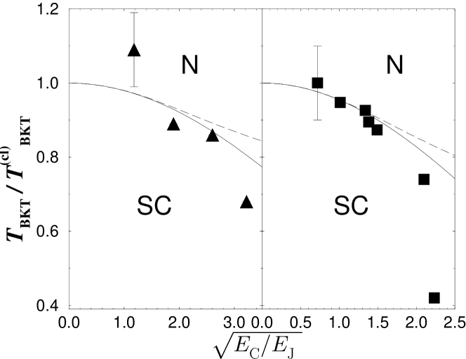
Figure 1: Experimental phase diagram for a JJA on triangular (left panel) and square (right panel) lattice [2]. The lower temperatures refer to the superconducting phase. The lines report the semiclassical result of the PQSCHA [4], in the limit $R_{{\rm{S}}}\gg R_{\rm Q}=h/(2e)^{2}$ with $\eta=10^{-2}$ (solid), and for strong dissipation, $R_{\rm Q}/R_{{\rm{S}}}=3$ (dashed).

Recently, fabricated arrays of nanosized junctions, both unshunted [3] and shunted [5], have given the opportunity to experimentally approach the quantum (zero-temperature) phase transition. However, the mechanism of suppression of the BKT in the neighborhood of the quantum critical point and its connection with the observed reentrance of the array resistance as function of the temperature is not yet clear [2, 3, 6]. In this paper we study the SC-N phase diagram by means of path-integral Monte Carlo (PIMC) [7, 8] simulations focusing the attention on the region of strong quantum fluctuations, in order to investigate their role in suppressing the BKT transition.

2 The model

The Josephson junction two-dimensional array (JJA) on the square lattice is modeled by a quantum $XY$ model with the following action:

$$S[\bm{\varphi}]=\int\limits_{0}^{\hbar\beta}\!\!\frac{du}{\hbar}\,\bigg{\{}\!\sum_{\bm{ij}}\frac{\hbar^{2}C_{\bm{ij}}}{8e^{2}}{\dot{\varphi}_{\bm{i}}(u)\,\dot{\varphi}_{\bm{j}}(u)}-E_{{}_{\rm J}}\sum_{\langle{\bm{ij}}\rangle}\cos\varphi_{\bm{ij}}(u)\bigg{\}},$$ (1)

where $\varphi_{\bm{ij}}=\varphi_{\bm{i}}-\varphi_{\bm{j}}$ is the phase difference between the Josephson phases on the $\bm{i}$th and the $\bm{j}$th neighboring superconducting islands. The capacitance matrix reads

$$C_{\bm{ij}}=C\,\Big{[}\eta\,\delta_{\bm{ij}}+\big{(}z\,\delta_{\bm{ij}}-{\sum}_{\bm{d}}\delta_{\bm{i},\bm{j+d}}\big{)}\Big{]}~{},$$ (2)

where $C_{0}\equiv\eta\,C$ and $C$ are, respectively, the self- and mutual capacitances of the islands, and $\bm{d}$ runs over the vector displacements of the $z\,{=}\,4$ nearest-neighbors. The standard samples of JJA are well decribed by the limits $\eta\ll{1}$, while for the granular films the opposite limits $\eta\gg{1}$ is more appropriate. The quantum dynamics of the system is determined by the Coulomb interaction between the Cooper pairs. This is described by the kinetic term through Josephson relation $\dot{\varphi}_{\bm{i}}=2eV_{\bm{i}}$. The Josephson coupling is represented by the cosine term, the latter favoring Cooper-pair tunneling across the junctions.

The quantum fluctuations are ruled by the quantum coupling parameter $g=\sqrt{E_{{}_{\rm{C}}}/E_{{}_{\rm{J}}}}$, where $E_{{}_{\rm{C}}}=(2e)^{2}/2C$ is the characteristic charging energy (for $\eta\ll{1}$). In the following we use the dimensionless temperature $t\equiv{k_{{}_{\rm B}}T/E_{{}_{\rm{J}}}}$. In our model Eq. (1) we assume the presence of very weak Ohmic dissipation due to the currents flowing to the substrate or through shunt resistances [5], which reflects into the prescription to consider the phase as an extended variable [2]. Apart from this, dissipative effects are negligible provided that the shunt resistance $R_{{}_{\rm{S}}}\gg{R_{{}_{\rm{Q}}}}\,g^{2}/(2\pi{t})$, where ${R_{{}_{\rm{Q}}}}\equiv{h/(2e)^{2}}$ is the quantum resistance; for smaller $R_{{}_{\rm{S}}}$ an explicit dissipative contribution should be added to the action (1), e.g. in the form of the Caldeira-Leggett term [2, 4],

$$S_{\rm CL}[\varphi]=\int\limits_{0}^{\hbar\beta}\frac{du}{2\hbar}\int\limits_{0}^{\hbar\beta}\,du^{\prime}\,\sum_{\bm{ij}}\,K_{\bm{ij}}(u-u^{\prime})\,\varphi_{\bm{i}}(u)\,\varphi_{\bm{j}}(u^{\prime})\,,$$ (3)

resulting in a decrease of quantum fluctuations. The two situations are the cases of the experiments in Ref. [3] and Ref. [5], respectively, where an increasing of the BKT transition temperature was found for increasing dissipation. This can be easily understood taking into account that the dissipative term (3) results from the coupling of the phase $\varphi_{\bm{i}}$ with environmental variables (the degrees of freedom of the dissipative bath), constituting an implicit measurement of $\varphi_{\bm{i}}$ .

3 Numerical simulations

Figure 2: Fitting parameter $A(t)$ for different values of $g$ ranging from $0.5$ to $3.0$. The BKT transition temperature is obtained by the condition $A(t_{{}_{\rm BKT}})\,{=}\,1$.

The numerical data for the BKT transition temperature are obtained using PIMC simulations on $L\times L$ lattices (up to $L=96$) with periodic boundary conditions. Thermodynamic averages are obtained by MC sampling of the partition function after discretization of the Euclidean time $u\in[0,\beta\hbar]$ in $P$ slices $\,\hbar\beta/P\,$, where $P$ is the Trotter number. However, the actual sampling is made on imaginary-time Fourier transformed variables on a lattice using the algorithm developed in Ref. [7]. The move amplitudes are independently chosen and dynamically adjusted for each Fourier component; this procedure turns out to be very efficient to reproduce the strong quantum fluctuations of the paths in the region of high quantum coupling  $g$. Indeed, test simulations with the standard PIMC algorithm showed serious problems of ergodicity, though eventually giving the same results. The approach through Fourier PIMC becomes more and more suitable and effective when dissipation is inserted, because the non-local action (3) becomes local in Fourier space. Additional details about the numerical method are given in the Appendix. An over-relaxation algorithm [9] over the zero-frequency mode has also been implemented in order to effectively reduce the autocorrelation times.

A very sensitive method to determine the transition temperature is provided by the scaling law of the helicity modulus $\Upsilon$ (a quantity proportional to the phase stiffness),

$$\Upsilon=\frac{1}{E_{{}_{\rm J}}}\left(\frac{\partial^{2}F}{\partial k_{0}^{2}}\right)_{k_{0}=0}~{},$$ (4)

which measures the response of the free energy $F$ (per unit volume) when a uniform twist $k_{0}$ along a fixed direction $\bm{u}$ is applied to the boundary conditions (i.e., $\varphi_{\bm{i}}\to\varphi_{\bm{i}}+k_{0}\bm{u}{\cdot}\bm{i}$, with the unitary vector $\bm{u}$).

Figure 3: Size scaling of the helicity modulus $\Upsilon_{L}$ at the transition temperature. Symbols are PIMC data and the dashed-lines are the one-parameter fit with Eq. (5), i.e. with $A(t)=1$. Left panel: $g=0$ and $t=0.892$ [$L_{0}=0.456(6)$]; right panel: $g=3.4$ and $t=0.25$ [$L_{0}=3.32(3)$]. The insets show $A(t)$ for different temperatures, using the two-parameter fit (see text).

The PIMC estimator for $\Upsilon$ is easily obtained, in analogy to that of Ref. [10], by derivation of the path-integral expression of the partition function (see Appendix). Kosterlitz’s renormalization group equations provide the critical scaling law for the finite-size helicity modulus $\Upsilon_{L}$:

$$\frac{\Upsilon_{L}(t_{{}_{\rm BKT}})}{t_{{}_{\rm BKT}}}=\frac{2}{\pi}\left(1+\frac{1}{2\ln(L/L_{0})}\right)~{},$$ (5)

where $L_{0}$ is a non-universal constant. Following Ref. [11], the critical temperature can be found by fitting $\Upsilon_{L}(t)/t$ vs $L$ for several temperatures according to Eq. (5) with a further multiplicative fitting parameter $A(t)$. In this way, the critical point can be determined by searching the temperature such that $A(t_{{}_{\rm BKT}})\,{=}\,1$, as illustrated in Figs 2 and 3. Using this procedure the critical temperature can be determined with excellent precision. For instance in the classical case we get $t_{{}_{\rm BKT}}(g{=}0)=0.892(2)$, in very good agreement with the most accurate results from classical simulations [12]. Also in the regime of strong quantum coupling, $g=3.4$, the PIMC data for $\Upsilon_{L}(t_{{}_{\rm{BKT}}}\,{=}\,0.25)$ are very well fitted by Eq. (5), as shown in Fig. 4. Moreover, this figure points out the sensitivity of this method to identify $t_{{}_{\rm{BKT}}}$: at temperature higher (lower) than the critical one the helicity modulus decreases (increases) much faster with $L$ than $\Upsilon_{L}(t_{{}_{\rm{BKT}}})$. At higher values of the quantum coupling, $g>g^{\star}$, the helicity modulus scales to zero with $L\to\infty$ and $P\to\infty$ at any temperature [8].

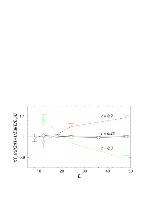
Figure 4: Helicity modulus $\Upsilon_{L}$ divided by the best fit with the expression (5) for $g\,{=}\,3.4$ and different temperatures: $\triangle$, $\bigcirc$, and $\square$ correspond to $t=0.2$, $0.25$, $0.3$, respectively.

Figure 5: Temperature behavior of the helicity modulus $\Upsilon_{8}(t)$ on a $8\,{\times}\,8$ lattice, for different values of $g$. The data are results from the Trotter extrapolation.

4 Results

We have found significant differences with the standard BKT theory. In the regime of strong quantum fluctuations, a range of coupling values, $3.2\lesssim{g}\lesssim{g^{\star}}$, is found in which the helicity modulus displays a non-monotonic temperature behavior.

In Fig. 5, $\Upsilon_{L}(t)$ is plotted for different values of $g$ on the $8\times 8$ cluster: up to $g=3.0$ it shows a monotonic behavior similar to the classical case, where thermal fluctuations drive the suppression of the phase stiffness. In contrast, for $g\,{=}\,3.4$, the helicity modulus is suppressed at low temperature, then it increases up to $t\sim 0.2$; for further increasing temperature it recovers the classical-like behavior and a standard BKT transition can still be located at $t\sim 0.25$ (Figs. 3 and 4). A reentrance of the phase stiffness was already found for a related model in Ref. [10], but the authors concluded that the drop of the helicity modulus at lowest temperatures was probably due to the finiteness of the Trotter number $\,P\,$.

Systematic extrapolations in the Trotter number and in the lattice size have been done, and presented in Figs. 7 and 7 for $g=3.4\,$, in order to ascertain this point. In particular, we did not find any anomaly in the finite-$P$ behavior: the extrapolations in the Trotter number appear to be well-behaved, in the expected asymptotic regime $\,{\cal O}(1/P^{2})\,$ [13], for $P\gtrsim 60$ (Fig. 7). Moreover, the extrapolation to infinite lattice-size shown in Fig. 7 clearly indicates that $\Upsilon_{L}$ scales to zero at $t=0.1$, while it remains finite and sizeable at $t=0.2$. therefore, the outcome of our analysis is opposite to that of Ref. [10], i.e., we conclude that the reentrant behavior of the helicity modulus appears to be a genuine effect present in the model, rather than a finite-Trotter or finite-size artifact.

Figure 6: Trotter-number extrapolation of $\Upsilon_{L}$ for $g=3.4$. Two series of data for $t=0.1$ ($\bullet$) and $0.2$ ($\blacksquare$) are reported, for four different lattice sizes: from the top to the bottom $L=8,10,12,14$. The lines are weighted quadratic fits.

Figure 7: Finite-size scaling of the helicity modulus $\Upsilon_{L}$ for $g=3.4$ at fixed $P=101$. The lines are guides for the eye.

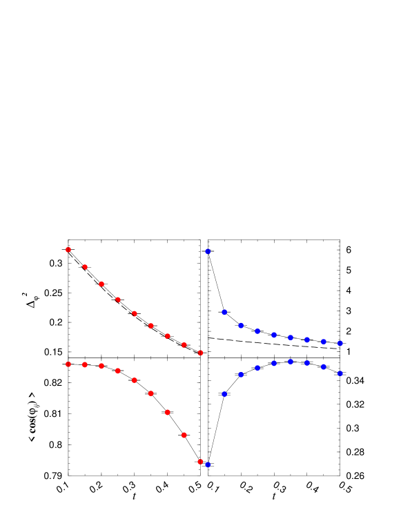
Figure 8: Top panels: $\Delta_{\varphi}^{2}$ vs $t$; bottom panels: $\langle\cos\,\varphi_{\bm{ij}}(u)\rangle$ vs $t$. The quantum coupling is $g=1.0$ in the left panels and $g=3.4$ in the right panels. The circles are PIMC data and the dashed lines are PQSCHA results.

In order to understand the physical reasons of the reentrance observed in the phase stiffness, we have studied the following two quantities:

$${\cal A} = \big{\langle}\,\cos\,\varphi_{\bm{ij}}(u)\,\big{\rangle}~{},$$ (6)

$$\Delta_{\varphi}^{2} = \big{\langle}\,(\varphi_{\bm{ij}}(u)-\bar{\varphi}_{\bm{ij}})^{2}\,\big{\rangle}~{},$$ (7)

with

$$\bar{\varphi}_{\bm{ij}}=\frac{1}{\hbar\beta}\int_{0}^{\hbar\beta}\!du~{}\varphi_{\bm{ij}}(u)\,$$ (8)

and $\bm{ij}\,$ nearest-neighbor sites. The first quantity $\,{\cal A}\,$, is a measure of the total (thermal plus quantum) short-range fluctuations of the Josephson phase and its maximum occurs where the overall fluctuations are lowest. The second quantity represents instead the pure-quantum spread of the phase difference between two neighboring islands and has been recently studied in the single junction problem [14]; more precisely, $\Delta_{\varphi}^{2}\,$ measures the fluctuations around the static value (i.e., the zero-frequency component of the Euclidean path), it is maximum at $t\,{=}\,0$ and tends to zero in the classical limit, i.e., $(g/t)\to{0}$.

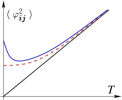
Figure 9: Qualitative picture of the behavior of the total mean square fluctuation of the nearest-neighbor phase difference. The straight line refer to the classical fluctuations. The lower (dashed) curve refers to the low-coupling case. The upper curve represents strongest couplings. $\langle\varphi_{\bm{ij}}^{2}\rangle$.

The quantities (6) and (7) on a $8\,{\times}\,8$ lattice are compared in Fig. 8 for two values of the quantum coupling, in the semiclassical ($g=1.0$) and in the extreme quantum ($g=3.4$) regime. In the first case $\,{\cal{A}}=\langle\cos\varphi_{\bm{ij}}(u)\rangle\,$ decreases monotonically by increasing $t$ and the pure-quantum phase spread $\Delta_{\varphi}^{2}$ shows a semiclassical linear behavior which is correctly described by the PQSCHA. At variance with this, at $g=3.4$, where the reentrance of $\Upsilon(t)$ is observed, $\,{\cal A}=\langle\cos\varphi_{\bm{ij}}(u)\rangle\,$ shows a pronounced maximum at finite temperature. Besides the qualitative agreement with the mean-field prediction of Ref. [15], we find a much stronger enhancement of the maximum above the $t\,{=}\,0$ value. This remarkable finite-$t$ effect can be explained by looking at $\Delta_{\varphi}^{2}(g{=}3.4)$ (Fig. 8, top-right panel). In fact its value is an order of magnitude higher than the one in the semiclassical approximation and, notably, it is strongly suppressed by temperature in a qualitatively different way from $\Delta_{\varphi}^{2}(g{=}1.0)$: i.e., the pure-quantum contribution to the phase fluctuations measured by $\Delta_{\varphi}^{2}$ decreases much faster than the linearly rising classical (thermal) one resulting in a global minimum of the total fluctuations. The qualitative behavior of the total mean square fluctuation of the nearest-neighbor phase difference vs. temperature is sketched in Fig. 9. This single-junction effect, in a definite interval of the quantum coupling ($3.2\lesssim{g}\lesssim 3.4$), is so effective to drive the reentrance of the phase stiffness. As for the transition in the region of high quantum fluctuations and low temperature, the open symbols in Figs. 10 and 11 represent the approximate location of the points $(t,g)$ where $\Upsilon(t)$ becomes zero within the error bars: in their neighborhood we did not find any BKT-like scaling law. This fact opens two possible interpretations: ($i$) the transition does not belong to the $XY$ universality class; ($ii$) it does, and in this case the control parameter is not the (renormalized) temperature, but a more involute function of both $t$ and $g$.

5 The phase diagram

Let us now describe our resulting phase diagram [8], displayed in Fig. 10 together with the semiclassical results valid at low coupling [4] and in Fig. 11 together with the experimental data [3] and our first PIMC outcomes including the dissipation effect.

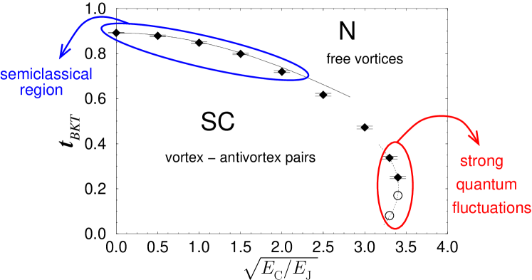
Figure 10: Phase diagram for a square lattice Josephson junction arrays in the limit $R_{{\rm{S}}}\gg R_{\rm Q}=h/(2e)^{2}$ with $\eta=10^{-2}$ . The symbols are our PIMC results and the line reports the semiclassical result of the PQSCHA [4].

At high temperature, the system is in the normal state with vanishing phase stiffness and exponentially decaying phase correlations, $\langle\varphi_{\bf{i}}\varphi_{\bf{j}}\rangle$. By lowering $t$, for $g\leq{g^{\star}}\,{\simeq}\,3.4$, the system undergoes a BKT phase transition at $t_{{}_{\rm{BKT}}}(g)$ to a superconducting state with finite stiffness and power-law decaying phase correlations. When $g$ is small enough (semiclassical regime), the critical temperature smoothly decreases by increasing $g$ and it is in remarkable agreement with the predictions of the pure-quantum self-consistent harmonic approximation (PQSCHA) [4]. For larger $g$ (but still $g<g^{\star}$) the semiclassical treatment becomes less accurate and the curve $t_{{}_{\rm BKT}}(g)$ shows a steeper reduction, but the SC-N transition still obeys the standard BKT scaling behavior. Finally, for $g>g^{\star}$ a strong quantum coupling regime with no sign of a SC phase is found. Surprisingly, the BKT critical temperature does not scale down to zero by increasing $g$ (i.e., $t_{{}_{\rm{BKT}}}(g^{\star})\neq{0}$): by reducing the temperature in the region $3.2\lesssim{g}\lesssim{g^{\star}}$, phase coherence is first established, as a result of the quenching of thermal fluctuations, and then destroyed again due to a dramatic enhancement of quantum fluctuations near $t=0$. This is evidenced by a reentrant behavior of the stiffness of the system, which vanishes at low and high $t$ and it is finite at intermediate temperatures. The open symbols in Fig. 10 mark the transition between the finite and zero stiffness region when $t$ is lowered.

When the interaction with a heat bath given by Eq.  (3) is present through a variable shunt resistance, the quantum phase fluctuations are decreased by the dissipation so that the BKT transition temperature rises. This is well reproduced by PQSCHA

Figure 11: Phase diagram for a square lattice Josephson junction arrays. Crossed circles are the experimental data [2]. The other filled symbols are our PIMC results, in the limit $R_{{\rm{S}}}\gg{R_{\rm{Q}}}=h/(2e)^{2}$ (diamonds), for $R_{\rm Q}/R_{{\rm{S}}}=0.25$ (squares) and $R_{\rm Q}/R_{{\rm{S}}}=0.5$ (circles), all with $\eta=10^{-2}$. The solid line reports the semiclassical non dissipative result of the PQSCHA [4].

approach [4] and turns out to be in qualitative agreement with recent experiments [5]. As shown in Fig. 11, the presence of intermediate ($R_{\rm Q}/R_{\rm S}=0.25$) and high ($R_{\rm Q}/R_{\rm S}=0.5$) dissipation causes the disappearance of the reentrance, in agreement with the experiments of Takahide et al. [5]. Their data do not show any anomalous reentrant behavior like those ones of the experiments on unshunted samples in Ref. [3]. Further investigations are needed to answer the question about the nature of the transition in the reentrance zone and to determine at which values of the dissipation the reentrant behavior is washed out.

6 Summary

In summary, we have studied a model for a JJA in the quantum-fluctuation dominated regime by means of Fourier path-integral Monte Carlo simulations. The BKT phase transition has been followed increasing the quantum coupling $g$ up to a critical value $g^{\star}\,{\sim}\,3.4$ where $t_{{}_{\rm BKT}}\sim 0.25$; above $g^{\star}$ no traces of BKT critical behavior have been observed. Remarkably, in the regime of strong quantum coupling ($3.2\lesssim{g}\lesssim 3.4$) phase coherence is established only in a finite range of temperatures, disappearing at higher $T$, with a genuine BKT transition to the normal state, and at lower $T$, due to a nonlinear quantum mechanism. This effect is destroyed by the presence of a relevant dissipation.

PIMC in the Fourier space for JJA

In this appendix we derive the discretized expressions of the observables to be measured by means of the simulations based on the Metropolis algorithm. The first step is to discretize the Euclidean time in $P$ slices, $u_{l}=(\hbar\beta/P)l$, and to perform a discrete Fourier transform

$$\varphi_{{\bm{i}},\alpha}=\frac{1}{P}\sum_{l=1}^{P}\varphi_{{\bm{i}},l}\,{\rm e}^{i\frac{2\pi}{P}l\alpha}~{},$$ (9)

where $\varphi_{{\bm{i}},l}=\varphi_{\bm{i}}(u_{l})$, and $\varphi_{{\bm{i}},\alpha}$ satisfies the conditions of periodicity, i.e. $\varphi_{{\bm{i}},\alpha}=\varphi_{{\bm{i}},\alpha+P}$, and reality of $\varphi_{{\bm{i}},l}$, i.e. $\varphi_{{\bm{i}},\alpha}=\varphi_{{\bm{i}},-\alpha}^{*}$. Thus the discretized path can be written as a sum over different frequency components

$$\varphi_{{\bm{i}},l}=\bar{\varphi}_{{\bm{i}}}+2\sum_{\alpha=1}^{N}\Re{\rm e}\left[\varphi_{{\bm{i}},\alpha}{\rm e}^{-i\frac{2\pi}{P}l\alpha}\right]=\bar{\varphi}_{{\bm{i}}}+2\sum_{\alpha=1}^{N}\left[a_{{\bm{i}},\alpha}\cos\frac{2\pi l\alpha}{P}+b_{{\bm{i}},\alpha}\sin\frac{2\pi l\alpha}{P}\right]~{},$$ (10)

where $\bar{\varphi}_{{\bm{i}}}$ is the zero-frequency component of the Euclidean path Eq. (8), and we choose an odd Trotter number $P=2N+1$. The advantage of using expression (10) is twofold. On the one hand the dissipative term of the action (3) that is non-local in time becomes diagonal. On the other hand the sampling can be performed independently on each frequency component, dynamically adjusting each move amplitude. This method make the sampling very effective especially in the region of strong quantum fluctuations, where the main contribution to the path comes from $\{a_{{\bm{i}},\alpha}\}$ and $\{b_{{\bm{i}},\alpha}\}$.

Using expression (10), the JJA action (1) plus the dissipative term (3) reads

$$S[{\bm{\varphi}}]=\sum_{\bm{ij}}\sum_{\alpha=1}^{N}T_{\bm{ij},\alpha}(a_{{\bm{i}},\alpha}a_{{\bm{j}},\alpha}+b_{{\bm{i}},\alpha}b_{{\bm{j}},\alpha})+\frac{\beta E_{{}_{\rm J}}}{P}\sum_{\langle\bm{ij}\rangle}\sum_{l=1}^{P}\big{(}1-\cos\varphi_{\bm{ij},l}\big{)}~{},$$ (11)

where $\varphi_{\bm{ij},l}=\varphi_{{\bm{i}},l}{-}\varphi_{{\bm{j}},l}$, and the “kinetic” matrix is

$$T_{\bm{ij},\alpha}=\frac{P^{2}}{\beta e^{2}}C_{\bm{ij}}\sin^{2}\frac{\pi\alpha}{P}+\beta K_{\bm{ij},\alpha}~{},$$ (12)

and $K_{\bm{ij},\alpha}$ is the discrete FT of the dissipative kernel matrix $K_{\bm{ij}}(u{-}u^{\prime})$. All the macroscopic thermodynamic quantities are obtained through the estimators generated from the discretized action (11). For instance the estimator of the helicity modulus $\Upsilon$ is obtained applying the definition (4) to the discretized free energy per unit volume

$$F=\frac{1}{\beta}\ln{\cal Z}=\frac{1}{\beta}\ln\left[C\int{\cal D}{\bm{\varphi}}\;{\rm e}^{-S[{\bm{\varphi}}]}\right]~{},$$ (13)

with the normalization constant $C$. Eventually we get

$$\Upsilon_{P} =t\Big{(}\frac{1}{\cal Z}\frac{\partial{\cal Z}}{\partial k_{0}}\Big{\arrowvert}_{k_{0}=0}\Big{)}^{2}-t\frac{1}{\cal Z}\frac{\partial^{2}{\cal Z}}{\partial k_{0}^{2}}\Big{\arrowvert}_{k_{0}=0}$$

$$=\frac{1}{P}\sum_{\langle\bm{ij}\rangle}\sum_{l=1}^{P}\cos\varphi_{\bm{ij},l}-\frac{1}{tP^{2}}\Big{(}\sum_{\langle\bm{ij}\rangle}\sum_{l=1}^{P}\sin\varphi_{\bm{ij},l}\Big{)}^{2}~{}.$$ (14)

11

References

- [1] V. L. Berezinskii, Zh. Eksp. Teor. Fiz. 59, 907 (1970) [Sov. Phys. JEPT 32, 493 (1971)]; J. M. Kosterlitz and D. J. Thouless, J. Phys. C 6, 1181 (1973).
- [2] R. Fazio and H. S. J. van der Zant, Phys. Rep. 355, 235 (2001).
- [3] H. S. J. van der Zant, W. J. Elion, L. J. Geerligs and J. E. Mooij, Phys. Rev. B 54, 10081 (1996).
- [4] A. Cuccoli, A. Fubini, V. Tognetti, and R. Vaia, Phys. Rev. B 61, 11289 (2000).
- [5] Y. Takahide, R. Yagi, A. Kanda, Y. Ootuka, and S. Kobayashi, Phys. Rev. Lett. 85, 1974 (2000).
- [6] H. M. Jaeger, D. B. Haviland, B. G. Orr, and A. M. Goldman, Phys. Rev. B 40, 182 (1989).
- [7] L. Capriotti, A. Cuccoli, A. Fubini, V. Tognetti, and R. Vaia, Europhys. Lett. 58, 155 (2002).
- [8] L. Capriotti, A. Cuccoli, A. Fubini, V. Tognetti, and R. Vaia, Phys. Rev. Lett. 91, 247004 (2003).
- [9] F. R. Brown and T. J. Woch, Phys. Rev. Lett. 58, 2394 (1987).
- [10] C. Rojas and J. V. José, Phys. Rev. B 54, 12361 (1996). (1994).
- [11] K. Harada and N. Kawashima, J. Phys. Soc. Jpn. 67, 2768 (1998); A. Cuccoli, T. Roscilde, V. Tognetti, R. Vaia, and P. Verrucchi, Phys. Rev. B 67, 104414 (2003).
- [12] P. Olsson, Phys. Rev. Lett. 73, 3339 (1994); M. Hasenbusch and K. Pinn, J. Phys. A 30, 63 (1997); S. G. Chung, Phys. Rev. B 60, 11761 (1999).
- [13] M. Suzuki, Quantum Monte Carlo methods in equilibrium and nonequilibrium systems, ed. M. Suzuki (Springer-Verlag, Berlin, 1987).
- [14] C. P. Herrero and A. Zaikin, Phys. Rev. B 65 104516 (2002).
- [15] P. Fazekas, B. Mühlschlegel, and Schröter, Z. Phys. B 57, 193 (1984).