Electron-nuclei spin relaxation through phonon-assisted hyperfine interaction
in a quantum dot

Abstract

We investigate the inelastic spin-flip rate for electrons in a quantum dot due to their contact hyperfine interaction with lattice nuclei. In contrast to other works, we obtain a spin-phonon coupling term from this interaction by taking directly into account the motion of nuclei in the vibrating lattice. In the calculation of the transition rate the interference of first and second orders of perturbation theory turns out to be essential. It leads to a suppression of relaxation at long phonon wavelengths, when the confining potential moves together with the nuclei embedded in the lattice. At higher frequencies (or for a fixed confining potential), the zero-temperature rate is proportional to the frequency of the emitted phonon. We address both the transition between Zeeman sublevels of a single electron ground state as well as the triplet-singlet transition, and we provide numerical estimates for realistic system parameters. The mechanism turns out to be less efficient than electron-nuclei spin relaxation involving piezoelectric electron-phonon coupling in a GaAs quantum dot.

I Introduction

Electron spin dynamics in mesoscopic devices has been attracting a lot of attention recently in the context of spintronics Wolf and quantum computation NCh ; DV . A crucial feature of this dynamics is the relaxation of the electron’s spin due to the interaction with an environment. Generally speaking, the coherence of an electronic spin state vanishes during the time $T_{2}$, which limits the possibility of coherent manipulation of qubits, while relaxation to thermal equilibrium occurs during another time $T_{1}$, which is usually larger than $T_{2}$ Abragam .

Several types of spin-dependent interactions can give rise to electron spin relaxation, e.g. the electron spin-orbit interaction PTreview ; Hasegawa ; Roth ; Frenkel ; KhN1 ; KhN2 ; MKGB ; WRL-G ; Tahan ; Glavin and the electron-nuclei hyperfine interaction Abragam ; DPreview ; PBS ; KimVX ; ENF ; EN ; Lyanda-Geller ; Sousa . Their action depends essentially on the dimension of the system. Systems of zero dimension, i.e. quantum dots (QDs), are characterized by a discrete electron energy spectrum. In this case energy conservation in the spin-flip process usually can be fulfilled only by transferring the energy to another subsystem, e.g. phonons. The energy transfer includes both the Zeeman energy of the electron spin in an external field and possibly the energy of an orbital transition. A discussion of other electron spin relaxation mechanisms not mentioned above and relevant to QDs can be found in Ref. KhN2, , for example. Electron spin relaxation in a QD due to hyperfine interaction alone, in the absence of an external magnetic field, was investigated recently in Refs. MER, ; SchKhL, .

Many years ago, the phonon-assisted electron spin-flip transition between Zeeman sublevels due to hyperfine interaction with an impurity nucleus and lattice nuclei was considered for impurity-bound electrons in silicon PBS , where the authors investigated the nuclear polarization in the Overhauser effect. The process that has been considered in that paper is associated with a crystal dilation and a corresponding adiabatic change in the electron effective mass and, as a consequence, in the electron envelope wave function and the hyperfine coupling constant. Recently, electron spin relaxation due to the hyperfine contact interaction has been readdressed with an application to GaAs QDs ENF ; EN . The transition amplitude was calculated in second-order perturbation theory, describing the action of the hyperfine contact interaction and a spin-independent piezoelectric electron-phonon coupling.

In this paper we will analyze another spin relaxation mechanism provided by the combination of hyperfine contact interaction and the influence of phonons on the electron inside a QD. In our approach we take into account directly the phonon-induced motion of nuclei which are coupled to the electron spin through the hyperfine interaction. The electron-phonon interaction appears via the displacement field shifting the positions of the nuclei, and therefore is independent of the piezoelectric coupling that applies only to crystals without inversion symmetry (such as GaAs, but not Si). Moreover, this mechanism allows the electron-nucleus spin flip-flop with a simultaneous emission of a phonon to appear already in first-order perturbation theory. Nevertheless, it will turn out that it is necessary to keep as well the second-order terms associated with the motion of the electron confining potential, since they lead to a crucial cancellation of first-order terms at low frequencies of the emitted phonon, thereby suppressing the relaxation rate. The physical reason behind this is the following: Long-wavelength phonons displace both the lattice nuclei and the electron’s confining potential in the same way. However, it is only the relative motion of the electron with respect to the nuclei that enables a transition. Therefore, the influence of long-wavelength phonons is suppressed. If, on the other hand, the confining potential can be considered as fixed or it moves independently from the lattice nuclei, this suppression does not apply any more, and the destructive interference between first-order and second-order terms is broken.

The present article is organized as follows: In Section II, we introduce the Hamiltonian of our model, including the effect of lattice vibrations on the hyperfine coupling and the confining potential. After that, we derive the electron spin flip transition amplitudes due to this perturbation, discussing the partial cancellation of terms and the dominating contribution. We calculate the transition rate, Eq. (23), for the case of Zeeman-split sublevels of the electron ground state (Sec. III), and perform an analogous derivation for the case of a triplet-singlet transition (Sec. IV). Finally, in Section V we look at numerical estimates for realistic system parameters.

II The model

In our model, we will assume the displacement of the QD confining potential to be described by the phonon displacement field evaluated at the center of the dot (which we take to be the origin). Note that this is analogous to the case of an impurity-bound electron. Any more detailed description (e.g. allowing for a distortion of the potential) would require further specifications concerning the way this potential is applied to the dot, but would not add significantly to the realism of the present model.

In the effective mass approximation the Hamiltonian of the system of electrons and phonons in the QD has the following form, if the perturbations due to electron-phonon and hyperfine interactions are excluded:

$$\!\!\hat{H}_{0}\!\! = \!\sum_{i}\left[\frac{\hat{{\bf P}}_{i}^{2}}{2m^{*}}+V({\bf r}_{i})+\text{g}^{*}\mu_{B}{\hat{\bf S}}_{i}\cdot{\bf B}\right]$$ (1)

$$+ \!\!\frac{1}{2}\sum_{i\neq i^{\prime}}V_{e-e}({\bf r}_{i}-{\bf r}_{{i}^{\prime}})+\!\!\sum_{\bf{k},\lambda}\hbar\omega_{\bf{k},\lambda}\!\left[\hat{b}^{\dagger}_{\bf{k},\lambda}\hat{b}_{\bf{k},\lambda}+\frac{1}{2}\right]\!,$$

where $\hat{{\bf P}}_{i}=-\text{i}\hbar{\bf\nabla}_{{\bf r}_{i}}+e{\bf A}({\bf r}_{i})/c$ is the kinematical momentum operator. This Hamiltonian describes interacting electrons with effective mass $m^{*}$ and effective g-factor g^∗, localized in a static external potential $V({\bf r})$, in the presence of a magnetic field ${\bf B}$ (with a corresponding vector potential ${\bf A}({\bf r})$), and free phonons. We neglect the Zeeman splitting of nuclear spin states, given the small value of the nuclear magnetic moment.

The hyperfine contact interaction of electrons of spin ${\bf\hat{S}}_{i}$ at positions ${\bf r}_{i}$ with nuclei of spin ${\bf\hat{I}}_{j}$ at positions ${\bf R}_{j}$ has the form [Abragam, ]:

$$\hat{V}_{H\!F}({\bf r}_{i}) = \sum_{j}\hat{V}_{h\!f}({\bf r}_{i}\!-\!{\bf R}_{j})$$ (2)

$$= Av_{0}\sum_{j}\hat{{\bf S}}_{i}\cdot\hat{{\bf I}}_{j}\;\delta({\bf r}_{i}-{\bf\hat{R}}_{j}),$$

where the hyperfine coupling constant is determined as

$$A=\frac{4\mu_{0}}{3I}\frac{\mu_{B}\mu_{I}}{v_{0}}\,\eta,$$ (3)

with $\eta=|u(0)|^{2}$ being the square of the Bloch amplitude at the site of the nucleus DPreview , $\mu_{B}>0$ the Bohr magneton, $\mu_{I}$ the nuclear magnetic moment, and $v_{0}$ the size of the unit cell. The factor $\eta$, which is usually of the order of $10^{2}$ to $10^{3}$, depending on the material, makes the Fermi contact term much more efficient than the other terms of the electron-nucleus hyperfine interaction Abragam . For a more complicated lattice structure the hyperfine constant $A$ is defined as a sum of the individual constants $A_{j}$ over all the nuclei in the unit cell, taking into account different values of spins and parameters $\eta$ for different nuclei DPreview .

The positions of the nuclei deviate slightly from equilibrium, due to the lattice vibrations: ${\bf\hat{R}}_{j}={\bf R}^{0}_{j}+{\bf\hat{u}}({\bf R}^{0}_{j})$. The lattice displacement field ${\bf\hat{u}}({\bf R}^{0}_{j})$ is described via the phonon creation-annihilation operators LL5 ,

$$\hat{{\bf u}}({\bf R}^{0}_{j})=\sum_{\bf{k},\lambda}\sqrt{\frac{\hbar}{2\rho\,\omega_{\bf{k},\lambda}V_{ph}}}(\hat{b}_{\bf{k},\lambda}+\hat{b}^{\dagger}_{\bf{-k},\lambda})\;{\bf\epsilon}_{\bf{k},\lambda}\;e^{\text{i}{\bf k}\cdot{\bf R}^{0}_{j}},$$ (4)

where ${\bf\epsilon}_{\bf{k},\lambda}$ is the polarization vector of a phonon with wave vector ${\bf k}$ in branch $\lambda$, $\omega_{\bf{k},\lambda}$ is its frequency, $V_{ph}$ is the volume of the crystal in which phonon modes are quantized, and $\rho$ is the crystal mass density.

As a consequence, the total Hamiltonian acquires the following term which can lead to a nucleus-electron spin flip-flop process combined with the emission of a phonon:

$$\hat{V}_{H\!F-ph}({\bf r}_{i})=-Av_{0}\!\sum_{j}\hat{{\bf S}}_{i}\cdot\hat{{\bf I}}_{j}\left(\hat{{\bf u}}({\bf R}^{0}_{j})\cdot\nabla_{{\bf r}_{i}}\right)\delta({\bf r}_{i}-{\bf R}^{0}_{j}).$$ (5)

In the following, we will omit the index $0$ for nuclear equilibrium positions.

Likewise, the vibrations of the confining potential are described by

$$\!\!\!\!\sum_{i}\delta\hat{V}({\bf r}_{i})=-\!\sum_{i}\left(\hat{{\bf u}}(0)\cdot{\bf\nabla}_{{\bf r}_{i}}\right)V({\bf r}_{i})$$ (6)

$$= \!\!\hat{{\bf u}}(0)\,[H_{0},\sum_{i}\frac{\text{i}}{\hbar}\hat{{\bf P}}_{i}]=-\frac{m^{*}}{\hbar^{2}}\hat{{\bf u}}(0)\!\sum_{i}\left[H_{0},[H_{0},{\bf r}_{i}]\right].$$

We note that the total electron momentum commutes with the electron-electron interaction potential.

Thus, the total perturbation to the Hamiltonian $\hat{H}_{0}$, Eq. (1), is given by the three terms described above:

$$\delta\hat{H}=\sum_{i}\left[\delta\hat{V}({\bf r}_{i})+\hat{V}_{H\!F}({\bf r}_{i})+\hat{V}_{H\!F-ph}({\bf r}_{i})\right].$$ (7)

III Transitions between Zeeman sublevels

At first, we will consider the transition of a single electron between the Zeeman-split spin levels of the QD ground state.

The initial state of the system is given by the direct product of electron, nuclear and phonon states:

$$|i\rangle=|i_{e}\rangle\otimes|i_{N}\rangle\otimes|i_{ph}\rangle.$$ (8)

Let ${\bf n}$ denote the direction of magnetic field. The initial electron state $|i_{e}\rangle=|\psi({\bf r})\rangle\otimes|{\bf n}_{-}\rangle$ is given by the product of the spin wave function $|{\bf n}_{-}\rangle$, which is an eigenfunction of the equation $({\bf n}\cdot\hat{{\bf S}})|{\bf n}_{\pm}\rangle=\pm\frac{1}{2}|{\bf n}_{\pm}\rangle$, and the properly normalized ground state coordinate wave function

$$\psi({\bf r})=\frac{1}{\sqrt{V}}\varphi_{0}({\bf r}),\;\;\;\;\;\;\;\frac{1}{V}\int d^{3}{\bf r}|\varphi_{0}({\bf r})|^{2}=1.$$ (9)

Here $V$ is the effective volume of the dot. In GaAs, where the electron g-factor is negative, the state $|{\bf n}_{-}\rangle$ corresponds to the maximum of energy. The initial nuclear spin state $|i_{N}\rangle$ is a direct product of states of all individual nuclei. We will average over the initial phonon field state in the end, by inserting mean phonon occupation numbers given by the Bose distribution function $n_{\omega}=1/(e^{\hbar\omega/k_{B}T}-1)$.

In the final state

$$|f\rangle=|f_{e}\rangle\otimes|f_{N}\rangle\otimes|f_{ph}\rangle,$$ (10)

the electronic spin points into the opposite direction, $|f_{e}\rangle=|\psi({\bf r})\rangle\otimes|{\bf n}_{+}\rangle$. Nuclear, $|f_{N}\rangle$, and phonon, $|f_{ph}\rangle$, final states are determined by the action of the perturbation potential $\hat{V}_{H\!F-ph}$ which changes the electron and nuclear spin states while conserving the total spin of the electron-nuclei system (flip-flop process) and creates a phonon with energy corresponding to the energy difference between electron initial and final states.

The corresponding transition matrix element is provided by first order perturbation theory in the potential $\hat{V}_{H\!F-ph}({\bf r})$:

$$\!\!\!\!\!\!\langle\!\!\! f \!\!\!\!|\delta{\hat{H}}|i\rangle^{(1)}$$ (11)

$$= \!\!\!-\!\sum_{j}\langle f_{ph}|\hat{\bf u}({\bf R}_{j})|i_{ph}\rangle\langle f_{e,N}|\nabla_{\bf r}\hat{V}_{h\!f}({\bf r}\!-\!{\bf R}_{j})|i_{e,N}\rangle.$$

It is important that an alternative process is possible for the transition between the same two states, where the remaining two terms in $\delta{\hat{H}}$ (namely $\delta{\hat{V}}$ and ${\hat{V}}_{HF}$) contribute in second order perturbation theory, yielding an amplitude that is of the same order of magnitude as Eq. (11):

$$\langle f|\delta{\hat{H}}|i\rangle^{(2)} = {\sum_{m}}^{\prime}\left[\frac{\langle f|\delta\hat{V}({\bf r})|m\rangle\langle m|\hat{V}_{H\!F}({\bf r})|i\rangle}{E_{i}^{(e)}-E_{m}^{(e)}}\right.$$ (12)

$$+ \left.\frac{\langle f|\hat{V}_{H\!F}({\bf r})|m\rangle\langle m|\delta\hat{V}({\bf r})|i\rangle}{E_{f}^{(e)}-E_{m}^{(e)}}\right],$$

where the sum is over all intermediate states which differ from the initial and final states, and $E^{(e)}$ refers to electron energies only. In writing down the energy denominators we have used the fact that the hyperfine perturbation only changes the electronic energies, and that initial and final total energies will be the same. Note that the complete electronic energy includes the Zeeman energy as well, and the difference between initial and final electron energies is accounted for by the energy of the emitted phonon, $\hbar\omega=E_{i}^{(e)}-E_{f}^{(e)}$.

Now we employ the expressions for the perturbation $\delta\hat{V}({\bf r})$, Eq. (6), in order to rewrite the previous formula in a form that displays the relation to the first order amplitude:

$$\langle\!\!\! f \!\!\!\!|\delta{\hat{H}}|i\rangle^{(2)}=\langle f_{ph}|\hat{\bf u}(0)|i_{ph}\rangle\left\{\langle f_{e,N}|\nabla_{\bf r}\hat{V}_{H\!F}({\bf r})|i_{e,N}\rangle\right.$$ (13)

$$- m^{*}\omega^{2}{\sum_{m}}^{\prime}\left[\frac{\langle f_{e,N}|\,{\bf r}\,|m_{e,N}\rangle\langle m_{e,N}|\hat{V}_{H\!F}({\bf r})|i_{e,N}\rangle}{E_{i}^{(e)}-E_{m}^{(e)}}\right.$$

$$+ \left.\left.\frac{\langle f_{e,N}|\hat{V}_{H\!F}({\bf r})|m_{e,N}\rangle\langle m_{e,N}|\,{\bf r}\,|i_{e,N}\rangle}{E_{f}^{(e)}-E_{m}^{(e)}}\right]\right\},$$

We have used the expressions for $\delta\hat{V}({\bf r})$ in terms of the commutator of $\hat{H}_{0}$ with both the kinematical momentum and the position operator, as well as the fact that $\hat{V}_{HF}$ commutes with the position.

The total amplitude of the transition is the sum of the terms (11) and (13). We will regroup it into two parts. The first one consists of Eq. (11) and a contribution of a similar form, the first term of Eq. (13),

$$A_{1}=\!\sum_{j}\langle f_{ph}|\hat{\bf u}(0)-\hat{\bf u}({\bf R}_{j})|i_{ph}\rangle\langle f_{e,N}|\nabla_{\bf r}\hat{V}_{h\!f}({\bf r}\!-\!{\bf R}_{j})|i_{e,N}\rangle.$$ (14)

It contains the difference between the phonon displacement fields evaluated at the origin and at the nucleus position, respectively, which is analogous to taking the divergence of the displacement field. This difference vanishes as $|\,{\bf k}{\bf R}_{j}|$ for long-wavelength phonons and describes the important cancellation which is only found if first and second orders of perturbation theory are combined properly.

The second part,

$$A_{2} = -\langle f_{ph}|\hat{\bf u}(0)|i_{ph}\rangle$$ (15)

$$\times m^{*}\omega^{2}{\sum_{m}}^{\prime}\left[\frac{\langle f_{e,N}|\,{\bf r}\,|m_{e,N}\rangle\langle m_{e,N}|\hat{V}_{H\!F}({\bf r})|i_{e,N}\rangle}{E_{i}^{(e)}-E_{m}^{(e)}}\right.$$

$$+ \left.\left.\frac{\langle f_{e,N}|\hat{V}_{H\!F}({\bf r})|m_{e,N}\rangle\langle m_{e,N}|\,{\bf r}\,|i_{e,N}\rangle}{E_{f}^{(e)}-E_{m}^{(e)}}\right]\right\},$$

contains a sum over intermediate states. For a single electron making a transition between the Zeeman sublevels of its ground state, we can set $E^{(e)}_{i}-E^{(e)}_{m}=\varepsilon_{0}-(\varepsilon_{m}-\hbar\omega)$ in the first summand and $E^{(e)}_{f}-E^{(e)}_{m}=(\varepsilon_{0}-\hbar\omega)-\varepsilon_{m}$ in the second. Note that in the two sums in Eq. (15) intermediate states with the same orbital energies $\varepsilon_{m}$ differ by the Zeeman energy.

In order to render the following discussion concrete, we will now specify the confining potential explicitly. We consider a QD which is formed in a two-dimensional electron gas (2DEG) by an external symmetric parabolic potential. The confining potential in z-direction is usually modelled by a square well in vertical QDs and by a triangular-shaped potential in lateral QDs. We neglect the contributions from higher excited states in the $z$-potential, given their large energetic separation, and restrict our discussion to the ground state $\chi_{0}(z)$. In the presence of an external magnetic field perpendicular to the $x-y$-plane, the electron wave functions in the lateral dimension become the Darwin-Fock solutions (see e.g. Ref. Kouwenhoven, ), with the effective confining frequency $\omega_{0}=\sqrt{\Omega_{0}^{2}+\omega_{c}^{2}/4}$, where $\Omega_{0}$ is the strength of the parabolic potential and $\omega_{c}=eB_{\perp}/(m^{*}c)$ the cyclotron frequency in an external magnetic field with the component $B_{\perp}$ perpendicular to the layer. The energy spectrum for these states is $\varepsilon_{n\lambda}=(2n+|\lambda|+1)\hbar\omega_{0}-\lambda\hbar\omega_{c}/2$.

In a harmonic oscillator the coordinate vector induces transitions only between nearest orbital levels. Thus, the sum in Eq. (15) reduces to two terms only corresponding to the transition from the ground state $\phi_{00}$ to states $\phi_{n\lambda}$, with $n=0$ and $\lambda=\pm 1$ being the radial and the angular momentum quantum numbers, respectively. For example, in cylindrical coordinates we rewrite the scalar product of the phonon polarization vector and the coordinate vector as ${\bf\epsilon}\,{\bf r}=(\epsilon_{+}\rho e^{-\text{i}\varphi}+\epsilon_{-}\rho e^{\text{i}\varphi})/\sqrt{2}$ and note that $\phi_{00}\rho e^{\pm\text{i}\varphi}/\sqrt{2}=l\,\phi_{0\,\pm 1}$, where $l=\sqrt{\hbar/(m^{*}\omega_{0})}$ is the length scale which determines the spatial extent of the electron wave function in the parabolic well in the presence of an external perpendicular magnetic field.

We now compare the two parts of the total amplitude that are given by Eqs. (14) and (15). First, we note that the matrix element $\langle f_{e,N}|\nabla_{\bf r}\hat{V}_{h\!f}({\bf r}\!-\!{\bf R}_{j})|i_{e,N}\rangle$ in the expression for $A_{1}$ is proportional to $|\nabla_{{\bf R}_{j}}\phi_{0}^{2}({\bf R}_{j})|$, where the gradient in the z-direction can be estimated as $\sim 1/z_{0}$, with $z_{0}$ the transverse dimension of the dot. Gradients in the lateral directions are smaller by a factor $z_{0}/l\ll 1$. The Zeeman splitting, $\hbar\omega=|\text{g}^{*}\mu_{B}B|$, is much less than the orbital energy splitting, $\hbar\omega\ll\hbar\omega_{0}$, in typical experiments on spin relaxation in QDs. Thus, up to a common prefactor, we can use the following estimates for the expressions of Eqs. (14) and (15):

$$|A_{1}|\propto\frac{\min[kl,1]}{z_{0}}\sim\frac{\min[\omega l/s,1]}{z_{0}},\;\;\;|A_{2}|\propto\frac{m^{*}\omega^{2}l}{\hbar\omega_{0}}\sim\frac{\omega^{2}}{\omega_{0}^{2}l},$$ (16)

where $s$ is the mean sound velocity. Finally, we find that the ratio $|A_{2}/A_{1}|$ is suppressed by a factor whose form depends on the emitted phonon wave-length:

$$\frac{z_{0}}{l}\frac{\omega}{\omega_{0}}\frac{s}{\omega_{0}l}\ll 1\;\;\;\;\text{for}\;\;\;\;kl\ll 1$$ (17)

$$\frac{z_{0}}{l}\left(\frac{\omega}{\omega_{0}}\right)^{2}\ll 1\;\;\;\;\text{for}\;\;\;\;kl\gg 1.$$

Taking this into account we will neglect $A_{2}$ in what follows.

Now we rewrite the total transition amplitude in the following, more explicit form (retaining only the main contribution):

$$\langle f|\delta{\hat{H}}|i\rangle^{(total)} = A\;\frac{v_{0}}{V}\;\sqrt{\frac{\hbar}{2\rho\,\omega_{\bf{k},\lambda}V_{ph}}}\;\sqrt{n_{\omega_{\bf{k},\lambda}}+1}$$ (18)

$$\times \sum_{j}\left(e^{\text{i}{\bf k}\cdot{\bf R}_{j}}-1\right)\hat{S}^{\alpha}_{+-}\,\langle f_{N}|\;\hat{I}^{\alpha}_{j}|i_{N}\rangle\;$$

$$\times ({\bf\epsilon}_{\bf{k},\lambda}\cdot{\bf\nabla}_{{\bf R}_{j}})\;\varphi_{0}^{2}({\bf R}_{j}),$$

where $\hat{S}^{\alpha}_{+-}=\langle{\bf n}_{+}|\hat{S}^{\alpha}|{\bf n}_{-}\rangle$ (a sum over $\alpha$ in Eq. (18) is assumed).

By means of Fermi’s golden rule we obtain the following expression for the transition rate (including a sum over final states and a proper average over initial states):

$$\dot{W} = \frac{2\pi}{\hbar}\frac{A^{2}}{N^{2}}\int\frac{d^{3}{\bf k}}{(2\pi)^{3}}\;\delta(\hbar\omega_{{\bf k}}-\hbar\omega)$$ (19)

$$\times \frac{\hbar}{2\rho\,\omega_{\bf k}}\,(n_{\omega_{\bf k}}+1)\sum_{j,j^{\prime}}F({\bf R}_{j},{\bf R}_{j^{\prime}})\;G_{jj^{\prime}}$$

$$\times \left[\,{\bf\nabla}_{{\bf R}_{j}}\varphi_{0}^{2}({\bf R}_{j})\cdot{\bf\nabla}_{{\bf R}_{j^{\prime}}}\varphi_{0}^{2}({\bf R}_{j^{\prime}})\,\right],$$

where $N=V/v_{0}$ is the number of unit cells inside the dot volume $V$. In (19) we have employed the sound wave dispersion law in the form $\omega_{\bf k}=ks$, i.e. we have neglected the difference in the transverse and longitudinal sound velocities in summation over phonon polarizations. This simplifies our formulas but should not change appreciably our numerical results.

For clarity, in Eq. (19) we have combined some exponential factors from Eq. (18) into the following expression:

$$F({\bf R}_{j},{\bf R}_{j^{\prime}})=4\,e^{\text{i}{\bf k}\cdot\frac{{\bf R}_{j}-{\bf R}_{j^{\prime}}}{2}}\sin\frac{{\bf k}\!\cdot\!{\bf R}_{j}}{2}\sin\frac{{\bf k}\!\cdot\!{\bf R}_{j^{\prime}}}{2}.$$ (20)

We have also separated all spin-related factors into the correlation function (cf. Refs. ENF, ; EN, ):

$$G_{jj^{\prime}}=\hat{S}^{\alpha}_{-+}\hat{S}^{\beta}_{+-}\langle i_{N}|\;\hat{I}^{\alpha}_{j}\,\hat{I}^{\beta}_{j^{\prime}}|i_{N}\rangle_{av},$$ (21)

where the subscript, av, indicates averaging over initial nuclear spin states (in our case over a thermal distribution).

At temperatures much higher than $\sim 10^{-7}\,K$, which is the order of magnitude of the nuclear spin-spin interaction, the nuclear spins are not correlated, i.e. $G_{jj^{\prime}}=G\,\delta_{jj^{\prime}}$. We suppose that there are no other sources of average nuclear polarization either. This means, in turn, that the interference terms in Eq. (19), stemming from different nuclei, $j\neq j^{\prime}$, vanish.

With the help of the usual commutation rules for spin components and the equality $\langle{\bf n}_{-}|\hat{{\bf S}}|{\bf n}_{-}\rangle=-\frac{1}{2}{\bf n}$, we obtain for each nuclear spin the formula

$$\hat{S}^{\alpha}_{-+}\hat{S}^{\beta}_{+-}\,\hat{I}^{\alpha}\,\hat{I}^{\beta}=\frac{1}{4}\left[\hat{{\bf I}}^{2}-(\hat{{\bf I}}\cdot{\bf n})^{2}+(\hat{{\bf I}}\cdot{\bf n})\right],$$ (22)

which results in a correlation function $G=\frac{1}{6}I(I+1)$, provided the average nuclear spin is zero.

Taking all of this into account, the following expression describes our main result for the rate of the electron-spin relaxation between Zeeman sublevels of the ground state, due to the hyperfine-phonon mechanism considered here:

$$\frac{1}{T_{1}} = \frac{A^{2}}{N}\frac{n_{\omega}+1}{6\pi\hbar\rho\,s^{3}}\;\omega\;I(I+1)$$ (23)

$$\times \overline{\left[1-\frac{\sin(k|{\bf R}^{\prime}|)}{k|{\bf R}^{\prime}|}\right]\left[{\bf\nabla}_{{\bf R}^{\prime}}\varphi_{0}^{2}({\bf R}^{\prime})\right]^{2}}.$$

The overbar in Eq. (23) indicates an average over the positions ${\bf R}^{\prime}$ of all nuclei in the dot. If the electron envelope wave function changes little on the scale of distance between the nuclei, then this is just a spatial average over an electron localization volume. In deriving Eq. (23), we have used the identity

$$\int\!d\Omega_{{\bf k}}\,\sin^{2}({\bf k}\cdot{\bf\xi})=2\pi\left[1-\frac{\sin(2k|{\bf\xi}|)}{2k|{\bf\xi}|}\right].$$ (24)

We note that the relaxation rate for an individual nuclear spin is obtained by dividing Eq. (23) by $N$.

IV Triplet-Singlet transition

We proceed in the same way in order to calculate the transition rate for two electrons that initially reside in the lowest-lying triplet state and decay towards the ground-state singlet. We suppose that the Zeeman splitting (produced by external and/or nuclear magnetic fields) can be neglected as compared to the orbital energy spacing that defines the transition energy for this process.

The wave function corresponding to the initial spin-triplet electron state is

$$|i_{e}^{T\!r}\rangle=|\psi^{T\!r}({\bf r}_{1},{\bf r}_{2})\rangle\otimes|T\!r\rangle,$$ (25)

where the coordinate wave function is assumed to be given by a Slater determinant (i.e. neglecting correlations):

$$\psi^{T\!r}({\bf r}_{1},{\bf r}_{2})=\frac{\varphi_{0}({\bf r}_{1})\varphi_{1}({\bf r}_{2})-\varphi_{0}({\bf r}_{2})\varphi_{1}({\bf r}_{1})}{V\sqrt{2}}\,.$$ (26)

Here $\varphi_{1}({\bf r})$ is the wave function of the first excited single electron orbital state normalized according to Eq. (9). For concreteness, we choose it to correspond to the quantum numbers $n=0$ and $\lambda=1$ (in an external magnetic field the energy of this state is less than $\varepsilon_{0,\,-1}$), and we note that there is no term in the total Hamiltonian which couples directly states with $\lambda=\pm 1$. We write for the spin part (as in Ref. ENF, )

$$|{T\!r}\rangle=-\frac{\nu_{x}-i\nu_{y}}{\sqrt{2}}|1,+1\rangle+\frac{\nu_{x}+i\nu_{y}}{\sqrt{2}}|1,-1\rangle+\;\nu_{z}|1,0\rangle,$$ (27)

where the coefficients $\nu_{x,y,z}$ determine the initial superposition of degenerate states $|S,m\rangle$ with different z-components $m=\pm 1,0$ of the total spin $S=1$ of two electrons.

For the final spin-singlet state we have

$$|f_{e}^{Si}\rangle=|\psi^{Si}({\bf r}_{1},{\bf r}_{2})\rangle\otimes|Si\rangle,$$ (28)

where $|Si\rangle$ denotes the singlet spin state ($S=0$), and the coordinate wave function is given by the expression:

$$\psi^{Si}({\bf r}_{1},{\bf r}_{2})=\frac{\varphi_{0}({\bf r}_{1})\varphi_{0}({\bf r}_{2})}{V}\,.$$ (29)

Again, the transition amplitude is given by Eqs. (14) and (15), where we have to introduce sums over electron coordinates: e.g. $\nabla_{\bf r}\hat{V}_{h\!f}({\bf r}\!-\!{\bf R}_{j})\rightarrow\sum_{i}\nabla_{{\bf r}_{i}}\hat{V}_{h\!f}({\bf r}_{i}\!-\!{\bf R}_{j})$, etc.

In the present case, the energy of the emitted phonon, $\hbar\omega$, is equal to the single-particle energy splitting, $\hbar\omega_{0}$. In the expression for $A_{2}$, Eq. (15), the contribution from the spin-singlet intermediate state dominates, due to the small denominator [ENF, ] given by the exchange splitting $\delta_{ST}$. However, although $\delta_{ST}$ is smaller than $\hbar\omega_{0}$, it still has the same order of magnitude ENF , and the ratio $|A_{2}/A_{1}|\sim(z_{0}/l)(\omega_{0}/\delta_{ST})$ is still much less than unity (here we have $kl\gg 1$). Therefore we can once more neglect $A_{2}$.

We obtain for the triplet-singlet transition rate:

$$\dot{W}^{ST}\!\!\! = \!\!\frac{2\pi}{\hbar}\frac{A^{2}}{N^{2}}\int\frac{d^{3}{\bf k}}{(2\pi)^{3}}\;\delta(\hbar\omega_{{\bf k}}-\hbar\omega)$$

$$\times \!\!\frac{\hbar}{2\rho\,\omega_{\bf{k}}}\,(n_{\omega_{{\bf k}}}+1)\sum_{j,j^{\prime}}F({\bf R}_{j},{\bf R}_{j^{\prime}})\;G_{jj^{\prime}}^{ST}$$

$$\times \!\!\frac{1}{2}\!\left[{\bf\nabla}_{{\bf R}_{j}}(\varphi_{0}({\bf R}_{j})\varphi_{1}({\bf R}_{j}))\cdot{\bf\nabla}_{{\bf R}_{j^{\prime}}}(\varphi_{0}({\bf R}_{j^{\prime}})\varphi_{1}({\bf R}_{j^{\prime}}))\right]\!\!,$$

where the correlation function is:

$$G_{jj^{\prime}}^{ST} = {\langle T|\hat{S}^{\alpha}_{1}-\hat{S}^{\alpha}_{2}|S\rangle\langle S|\hat{S}^{\beta}_{1}-\hat{S}^{\beta}_{2}|T\rangle}\langle i_{N}|\;\hat{I}^{\alpha}_{j}\cdot\hat{I}^{\beta}_{j^{\prime}}|i_{N}\rangle_{av}$$ (31)

$$= \!{\nu^{*\alpha}\nu^{\beta}}\langle i_{N}|\;\hat{I}^{\alpha}_{j}\cdot\hat{I}^{\beta}_{j}|i_{N}\rangle_{av}\delta_{jj^{\prime}}=\frac{1}{3}I(I+1)\delta_{jj^{\prime}}.$$

Again, the nuclear spin state is averaged over a completely unpolarized thermal distribution.

Finally, the relaxation rate in this case is:

$$\!\!\!\!\!\frac{1}{T^{ST}_{1}}\!\!\! = \!\frac{A^{2}}{N}\frac{n_{\omega}+1}{6\pi\hbar\rho\,s^{3}}\;\omega\;I(I+1)$$ (32)

$$\times \!\!\!\overline{\left[1-\frac{\sin(k|{\bf R}^{\prime}|)}{k|{\bf R}^{\prime}|}\right]\!\!\left[{\bf\nabla}_{{\bf R}^{\prime}}\left(\varphi_{0}({\bf R}^{\prime})\varphi_{1}({\bf R}^{\prime})\right)\right]^{2}}.$$

V Numerical estimates and discussion

In order to estimate the rates in both of the cases that have been considered above, we take into account realistic dimensions of typical quantum dots. Usually the lateral length of the dot is much larger than its transverse dimension, $l\gg z_{0}$, and we use the following approximation: $\left[{\bf\nabla}_{{\bf R}^{\prime}}\left(\varphi_{0}({\bf R}^{\prime})\varphi_{1}({\bf R}^{\prime})\right)\right]^{2}\simeq\left[{\bf\nabla}_{{\bf R}^{\prime}}\varphi_{0}^{2}({\bf R}^{\prime})\right]^{2}\simeq\frac{1}{(z_{0}/2)^{2}}$ (which we suppose holds for the average over nuclear positions ${\bf R}^{\prime}$). For QDs with a disc shape, in the typical limit $kz_{0}<1$, we can obtain a simple analytical expression for the average,

$$f(kl)\equiv\overline{\left[1-\frac{\sin(k|{\bf R}^{\prime}|)}{k|{\bf R}^{\prime}|}\right]}\simeq 1-\frac{2(1-\cos(kl))}{(kl)^{2}},$$ (33)

which can be well approximated by $\min\{(kl)^{2}/12,1\}$. We remark that this factor, which is present in the case of the co-moving confining potential, is absent when the confining potential position is fixed. This is the only difference in the results for the relaxation rates in these two cases, and it becomes important only in the limit of small phonon frequencies, $kl\ll 1$.

We can write the relaxation rate between Zeeman sublevels and triplet and singlet electron states using the same approximate expression (the difference lies in the energy scale $\omega$):

$$\frac{1}{T_{1}}\simeq\frac{2}{3}\,\frac{A^{2}}{N}\;\frac{\omega\,(n_{\omega}+1)}{\pi\hbar\,\rho\,s^{3}z_{0}^{2}}I(I+1)\,f(kl).$$ (34)

The linear dependence of the relaxation rate on the phonon frequency (for phonon wave lengths smaller than the size of the QD, i.e. for sufficiently strong magnetic fields in the case of Zeeman sublevels relaxation) sets our mechanism apart from those considered earlier PBS ; EN , where a cubic phonon frequency dependence is expected for low temperatures, $k_{B}T\ll\hbar\omega$ (and a quadratic one in the opposite limit). In addition, our result does not depend either on the proximity of the nearest level, in contrast to the spin relaxation rates calculated in Refs. ENF, ; EN, .

The result for the electron-nuclei flip-flop transition rate obtained in Ref. PBS, is larger than our result, Eq. (34), by a factor $\sim(\gamma z_{0}/l)^{2}$ (provided $kl\ll 1$), which is of the order of $10$ ($\gamma\simeq 50$) for typical QD sizes cited below, but can be smaller for large QDs. We should be cautious, however, in applying directly the reasoning of Ref. PBS, to the triplet-singlet transition, when the emitted phonon energy corresponds to the electron binding energy and hence the condition of adiabatic electron motion in a vibrating lattice (used in that work) will not be fulfilled.

In GaAs all nuclei have spin $I=\frac{3}{2}$, and $A$ is the sum of $A_{j}$ over all the nuclei in the unit cell: $A=\sum_{j}A_{j}\simeq 90$ $\mu$eV DPreview . The mass density is $\rho\simeq 5.32\times 10^{3}$ kg/m³, and we approximate the mean sound velocity by the velocity of transverse sound waves, $s\sim s_{t}\simeq 3\times 10^{3}$ m/s Adachi . The typical transverse dimension of a quantum dot is $z_{0}\simeq 10$ nm and its lateral size is $l\simeq 100$ nm. The dot contains about $N\sim 10^{5}$ unit cells (8 nuclei in each). Hence, we can write for the relaxation rate the approximate expression:

$$\frac{1}{T_{1}}\simeq 1\times 10^{-15}\frac{\omega}{1-\exp(-\frac{\hbar\,\omega}{k_{B}T})}\,f(kl).$$ (35)

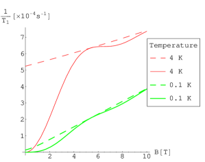
Figure 1: The single electron spin relaxation rate in a GaAs QD versus magnetic field (according to Eq. (35)), derived for the hyperfine-phonon mechanism discussed in the present article. The solid line corresponds to the case when the confining potential vibrates together with the lattice, while the dashed line refers to the case of a fixed confining potential.

For the transition between Zeeman energy sublevels the phonon energy is equal to the Zeeman splitting, $|\text{g}^{*}\mu_{B}B|$, which corresponds to $0.025$ meV T^-1 in GaAs where $\text{g}^{*}=-0.44$. At the same time the cyclotron energy, $\hbar\omega_{c}$, is as much as $1.76$ meV T^-1 due to the small effective mass in GaAs, $m^{*}=0.067m_{e}$. Consequently, the condition $\omega\ll\omega_{0}$ is always satisfied when a perpendicular magnetic field is applied. For in-plane magnetic fields $\omega\ll\omega_{0}$ when $B\ll 10$ T in a lateral and $B\ll 100$ T in a vertical QD (the single particle energy spacing in a lateral QD is 100 - 300 $\mu$eV, and in a vertical QD the confining energy of an approximate 2D harmonic potential is $\sim 4$ meV Kouwenhoven ; FujiPhys ). The condition $kl\sim 1$ corresponds to a magnetic field of the order of $1$ T. Thus, for magnetic fields larger than $\sim 1$ T the relaxation rate is linear in the emitted phonon frequency and as a consequence it is linear in the strength of the magnetic field (see Fig. (1) which is plotted for the limit $kz_{0}<1$ corresponding to $B<10$ T). For the fixed or ”independent” confining potential we would have $f(kl)\equiv 1$ and the dependence of the rate on the emitted phonon frequency would be linear even for small magnetic fields, i.e. when $kl\ll 1$ (apart from the temperature-dependent factor $(n_{\omega}+1)$).

As to the order of magnitude, the mechanism that has been considered in this paper gives a rate of the order of $10^{-4}$ s^-1 for a temperature of about 1 K and a magnetic field of about 1 T. It therefore appears to be much less efficient than the piezoelectric coupling mechanism considered in Ref. EN, , where the rate is about 1 s^-1 for comparable values of temperature, 4 K, and magnetic field, 0.5 T.

For the triplet-singlet transition in a lateral dot we find a rate of the order of $10^{-4}$ s^-1 for temperatures up to $\sim 1\,K$ ($\hbar\omega\sim 100\mu$eV), and in a vertical QD we have $1/T_{1}\sim 10^{-3}$ s^-1 for temperatures up to $\sim 10$ K and $\hbar\omega\sim 1$ meV (we note that in both cases $kl\gg 1$). The latter result should be compared with $1/T_{1}\approx 2\times 10^{-2}$ s^-1 calculated in Ref. ENF, .

Let us now turn to spin relaxation in silicon. Taking into account the natural abundance of ²⁹Si nuclei with non-zero spin $n_{I=1/2}=4.68\%$, their magnetic moment $\mu_{I}=-0.56\,\mu_{N}$, the lattice constant $a=5.43$ Å  and the electronic density at the position of the nucleus $\eta\simeq 186$ Abragam we find the effective hyperfine coupling constant to be $A\simeq 5$ $\mu$eV. This is far smaller than in GaAs, due to the smaller $\eta$ and smaller percentage of nuclei with spin. Inserting the mass density of Si, $\rho\simeq 2.3\times 10^{3}$ kg/m³ and the transverse sound velocity $s_{t}\simeq 5.4\times 10^{3}m/s$, we obtain a prefactor of the order of $10^{-20}$ in Eq. (35). This corresponds to a very small relaxation rate $1/T_{1}\sim 10^{-9}$ s^-1 between Zeeman sublevels in a magnetic field of $B=1$ T, for temperatures up to 1 K (g = 2 in Si). Note that the spin-orbit related electron spin relaxation time in lateral Si QDs Glavin , for Si:P bound electrons and for QDs in SiGe heterostructures Tahan has been predicted recently to be on the order of several minutes for the same values of magnetic field and temperature. In the latter case, however, the relaxation rate may be strongly decreased, below the values found for our mechanism, by application of uniaxial compressive strain Tahan .

In general, electron spin relaxation induced by electron-nuclei hyperfine interaction in a quantum dot is not as efficient as relaxation due to spin-orbit interaction for typical values of system parameters KhN1 ; KhN2 ; WRL-G ; MKGB ; Tahan ; Glavin ; ENF . In many experiments, the hyperfine related rate would be masked by the spin-orbit mechanism (However, see Ref. EN, for a case where the hyperfine mechanism may dominate). The present experimental data for the triplet-singlet transition rate in a GaAs vertical QD is $T_{1}\approx 200\mu$s at temperatures up to 0.5 K and triplet-singlet energy splitting $\varepsilon_{S-T}\sim 0.6$ meV FujiNature . For the relaxation time between Zeeman sublevels in a lateral GaAs QD only a lower bound is available: $T_{1}\gtrsim$ 50 $\mu$s for an in-plane magnetic field B=7.5 T at T=20 mK Hanson . Both of these measurement results were obtained by means of transient current spectroscopy FujiPRB .

On the other hand, hyperfine coupling mechanisms (such as the one considered in this paper) may be particularly relevant as far as effects like dynamic nuclear polarization are concerned, where the electron-nuclei hyperfine interaction plays a crucial role Abragam ; DPreview ; PBS . Recently, a hyperfine nuclear spin relaxation time on the order of 10 min was measured in a single GaAs QD, at a bath temperature of 40 mK and a magnetic field up to 0.5 T Huttel . However, this experiment dealt with a nonequilibrium transport situation, with a resulting spin-flip mechanism whose rate turns out to be orders of magnitude larger than the one discussed in the present article (see Ref. Lyanda-Geller, ).

VI Conclusions

In summary, we have considered a specific mechanism for inelastic electron spin relaxation in a QD induced by the electron-nuclei hyperfine interaction in combination with lattice vibrations. We have found that the interference between first and second orders of perturbation theory is essential for a correct description of the suppression of relaxation at small transition frequencies. The relaxation rate has been calculated both for the transition between Zeeman sublevels of the orbital ground state and for the triplet-singlet transition. We have obtained estimates based on these general results and realistic system parameters. The estimates demonstrate that the relaxation rate due to this particular mechanism is very small: For the spin relaxation between Zeeman sublevels it is much less than the rate calculated earlier in second order perturbation theory with an emission of a phonon through piezoelectric electron-phonon coupling in a GaAs QD EN , and it is less than (or at most comparable with) the relaxation rate due to the change in the localized electron effective mass induced by the lattice dilation in silicon PBS . For the triplet-singlet transition, the rate in GaAs QDs is still smaller by an order of magnitude than the corresponding rate of the piezoelectric mechanism.

We would like to thank B. L. Altshuler, D. V. Averin, C. Bruder, E. V. Sukhorukov and A. V. Chaplik for useful discussions.

References

- (1) S. A. Wolf et al., Science 294, 1488 (2001).
- (2) M. A. Nielsen and I. L. Chuang, Quantum Computation and Quantum Information (Cambridge University Press, Cambridge, New York, 2000).
- (3) D. P. DiVincenzo, Fortschr. Phys. 48, 771 (2000).
- (4) A. Abragam, The principles of nuclear magnetism (Oxford University Press 1961), Chapters VI, IX.
- (5) G. E. Picus and A. N. Titkov, in Optical Orientation, edited by F. Meier and B. P. Zakharchenya (Elsevier, Amsterdam, 1984).
- (6) H. Hasegawa, Phys. Rev. 118, 1523 (1960).
- (7) L. M. Roth, Phys. Rev. 118, 1534 (1960).
- (8) D. M. Frenkel, Phys. Rev. B 43, 14228 (1991).
- (9) A. V. Khaetskii and Y. V. Nazarov, Phys. Rev. B 61, 12639 (2000).
- (10) A. V. Khaetskii and Y. V. Nazarov, Phys. Rev. B 64, 125316 (2001).
- (11) L. M. Woods, T. L. Reinecke, and Y. Lyanda-Geller, Phys. Rev. B 66, 161318(R) (2002).
- (12) D. Mozyrsky, S. Kogan, V. N. Gorshkov, and G. P. Berman, Phys. Rev. B 65, 245213 (2002).
- (13) Ch. Tahan, M. Friesen, and R. Joynt, Phys. Rev. B 66, 035314 (2002).
- (14) B. A. Glavin and K. W. Kim, Phys. Rev. B 68, 045308 (2003).
- (15) M. I. Dyakonov and V. I. Perel, in Optical Orientation, edited by F. Meier and B. P. Zakharchenya (Elsevier, Amsterdam, 1984).
- (16) D. Pines, J. Bardeen, and C. P. Slichter, Phys. Rev. 106, 489 (1957).
- (17) J. H. Kim, I. D. Vagner, and L. Xing, Phys. Rev. B 49, 16777 (1994).
- (18) S. I. Erlingsson, Y. V. Nazarov, and V. I. Fal’ko, Phys. Rev. B 64, 195306 (2001).
- (19) S. I. Erlingsson and Y. V. Nazarov, Phys. Rev. B 66, 155327 (2002).
- (20) Y. B. Lyanda-Geller, I. L. Aleiner, and B. L. Altshuler, Phys. Rev. Lett. 89, 107602 (2002).
- (21) R. de Sousa and S. Das Sarma, Phys. Rev. B 68, 115322 (2003).
- (22) I. A. Merkulov, Al. L. Efros, and M. Rosen, Phys. Rev. B 65, 205309 (2002).
- (23) J. Schliemann, A. Khaetskii, and D. Loss, J. Phys.: Condens. Matter 15, R1809 (2003).
- (24) L. D. Landau and E. M. Lifshitz, Statistical Physics, Part 1 (Pergamon Press Ltd 1980).
- (25) L. P. Kouwenhoven, D. J. Austing, and S. Tarucha, Rep. Prog. Phys. 64(3), 701 (2001).
- (26) S. Adachi, J. Appl. Phys. 58(3), R1 (1985).
- (27) T. Fujisawa et al., Physica B 314, 224 (2002).
- (28) T. Fujisawa, Y. Tokura, and Y. Hirayama, Phys. Rev. B 63, 081304(R) (2001).
- (29) T. Fujisawa et al., Nature (London) 419, 278 (2002).
- (30) R. Hanson et al., Phys. Rev. Lett. 91, 196802 (2003).
- (31) A. K. Hüttel et al., cond-mat/0308243.